Nodal Structure of Superconductors with Time-Reversal Invariance
and ${\bm{Z}}_{2}$ Topological Number

Abstract

A topological argument is presented for nodal structures of superconducting states with time-reversal invariance. A generic Hamiltonian which describes a quasiparticle in superconducting states with time-reversal invariance is derived, and it is shown that only line nodes are topologically stable in single-band descriptions of superconductivity. Using the time-reversal symmetry, we introduce a real structure and define topological numbers of line nodes. Stability of line nodes is ensured by conservation of the topological numbers. Line nodes in high-$T_{\rm c}$ materials, the polar state in $p$-wave paring and mixed singlet-triplet superconducting states are examined in detail.

I Introduction

Nontrivial nodal structures are one of the most noticeable features of unconventional superconducting gap functions. Conventionally, the nodal structures have been investigated by power law behaviours of the temperature dependences of the specific heat, the NMR relaxation rates and so on Leggett (1975); Sigrist and Ueda (1991). Although the power law behaviours give a hint of the nodal structures, they can not give the details such as the number and the position of nodes. Recently, it has been increasingly clear that the angular-controlled measurements of thermal conductivity and specific heat in a vortex state are useful probes to determine the details of the nodal structures Volovik (1993); Vekhter et al. (1999); Won and Maki (2001). Various unexpected nodal structures of superconductors have been found in this method Aubin et al. (1997); Izawa et al. (2001a, b, 2002a, 2002b, 2003, 2005); Tanatar et al. (2001a, b); Deguchi et al. (2004a, b); Aoki et al. (2004); Park et al. (2003, 2004); Parks et al. (2004). This makes urgent the need for a better theoretical understanding of nodal structures of superconductors.

The purpose of this paper is to reveal theoretically a generic nodal structure of superconducting states with time-reversal invariance. We use two different methods to investigate the nodal structures. The first one is based on a universal Hamiltonian we will construct, and the other is an argument using topological numbers in momentum space. Unless stated explicitly, our results do not rely on any specific symmetry of superconducting states except the time-reversal symmetry.

Topological arguments in momentum space are powerful tools to investigate a nonperturbative aspect of quantum theories Nilesen and Ninomiya (1981); Thouless et al. (1982); Berry (1984); Kohmoto (1985). For superconducting states with broken time-reversal invariance, a topological characterization of the nodal structures was given in Refs.Volovik (1987, 2001); Hatsugai et al. (2004). On the other hand, we will present here a topological characterization of nodal structures of superconducting states with time-reversal invariance. We will introduce novel topological numbers and discuss stability of the nodal structures.

The organization of this paper is as follows. In Sec.II, we derive a generic Hamiltonian describing a quasiparticle in superconducting states with time-reversal invariance. The quasiparticle spectra are given and their nodal structures are discussed. In Sec.III, we examine stability of line nodes for high-$T_{\rm c}$ materials, the polar state in $p$-wave paring, and mixed singlet-triplet states, respectively. In Sec.IV, a real structure is introduced and novel ${\bm{Z}}_{2}$ topological numbers of line nodes are defined. We calculate the ${\bm{Z}}_{2}$ topological numbers for high-$T_{\rm c}$ materials, the polar state in $p$-wave paring, and mixed singlet-triplet states. It is shown that the existence of the topological numbers ensures stability of the line nodes. Conclusions and discussions are given in Sec.V.

II Hamiltonian with time-reversal symmetry and nodal structure

We derive here a generic Hamiltonian which describes a quasiparticle in superconducting states with time-reversal invariance. Let us consider a single-band description of superconducting state and start with the following Bogoliubov-de Gennes type Hamiltonian,

$$H=\frac{1}{2}\sum_{\bm{k}}{\bm{c}}({\bm{k}})^{\dagger}H({\bm{k}}){\bm{c}}({\bm{k}}),$$ (1)

where ${\bm{c}}({\bm{k}})$ is a four component notation of electron creation and annihilation operators in momentum space,

$${\bm{c}}({\bm{k}})=\left(\begin{array}[]{c}c_{\sigma}({\bm{k}})\\ c_{\sigma}(-{\bm{k}})^{\dagger}\end{array}\right),\quad(\sigma=\pm),$$ (4)

and $H({\bm{k}})$ is a $4\times 4$ Hermitian matrix which will be determined below. Since ${\bm{c}}({\bm{k}})$ satisfies

$${\bm{c}}(-{\bm{k}})^{*}=\Gamma{\bm{c}}({\bm{k}}),\quad\Gamma=\left(\begin{array}[]{cc}0&1\\ 1&0\end{array}\right),$$ (7)

we can set the matrix $H({\bm{k}})$ to satisfy the following equation,

$$\Gamma H({\bm{k}})\Gamma=-H(-{\bm{k}})^{*}.$$ (8)

We also demand that the Hamiltonian is time-reversal invariant. The time-reversal operation ${\cal T}$ is defined as

$${\cal T}{\bm{c}}({\bm{k}})=\Theta{\bm{c}}(-{\bm{k}})^{*},\quad\Theta=\left(\begin{array}[]{cc}i\sigma_{2}&0\\ 0&i\sigma_{2}\end{array}\right),$$ (11)

where $\sigma_{i}$’s $(i=1,2,3)$ are the Pauli matrices. Time-reversal invariance of $H$ implies

$$\Theta H({\bm{k}})\Theta^{-1}=H(-{\bm{k}})^{*}.$$ (12)

We solve Eqs.(8) and (12) to obtain a generic Hamiltonian of a quasiparticle in superconducting states with time-reversal invariance.

To solve Eq.(12), we rewrite the 16 components of $H({\bm{k}})$ in terms of the identity matrix, 5 Dirac matrices $\Gamma_{a}$ and 10 commutators $\Gamma^{ab}=[\Gamma_{a},\Gamma_{b}]/(2i)$ Kane and Mele (2005),

$$H({\bm{k}})=h_{0}({\bm{k}})1+\sum_{a=1}^{5}h_{a}({\bm{k}}){\Gamma_{a}}+\sum_{a<b=1}^{5}h_{ab}({\bm{k}})\Gamma_{ab}.$$ (13)

Here $h_{0}({\bm{k}})$, $h_{a}({\bm{k}})$’s and $h_{ab}({\bm{k}})$’s are real functions of ${\bm{k}}$. We choose the following representation of $\Gamma_{a}$,

$$\Gamma_{1}=\left(\begin{array}[]{cc}0&1\\ 1&0\end{array}\right),\quad\Gamma_{2}=\left(\begin{array}[]{cc}1&0\\ 0&-1\end{array}\right),$$ (18)

$$\Gamma_{3}=\left(\begin{array}[]{cc}0&-i\sigma_{1}\\ i\sigma_{1}&0\end{array}\right),\quad\Gamma_{4}=\left(\begin{array}[]{cc}0&-i\sigma_{2}\\ i\sigma_{2}&0\end{array}\right),$$ (23)

$$\Gamma_{5}=\left(\begin{array}[]{cc}0&-i\sigma_{3}\\ i\sigma_{3}&0\end{array}\right).$$ (26)

In this representation, we obtain

$$\Theta\Gamma_{a}\Theta^{-1}=\Gamma_{a}^{*},\quad\Theta\Gamma_{ab}\Theta^{-1}=-\Gamma_{ab}^{*}.$$ (27)

Therefore, Eq.(12) is satisfied if we have

$$h_{0}({\bm{k}})=h_{0}(-{\bm{k}}),\quad h_{a}({\bm{k}})=h_{a}(-{\bm{k}}),$$ (28)

and

$$h_{ab}({\bm{k}})=-h_{ab}(-{\bm{k}}).$$ (29)

In addition to Eq.(12), we impose Eq.(8) on Eq.(13). Using $\Gamma=\Gamma_{1}$ and the commutation relation of $\Gamma_{a}$’s, we find that the following 8 functions should be identically zero,

$$h_{0}({\bm{k}})=h_{1}({\bm{k}})=h_{3}({\bm{k}})=h_{5}({\bm{k}})=0,$$

$$h_{13}({\bm{k}})=h_{15}({\bm{k}})=h_{24}({\bm{k}})=h_{35}({\bm{k}})=0.$$ (30)

Therefore, the Hamiltonian contains 16-8=8 independent functions. It is convenient to introduce a new notation of the remaining functions,

$$h_{2}({\bm{k}})=\epsilon({\bm{k}}),\quad h_{4}({\bm{k}})=-\psi({\bm{k}}),$$

$$(h_{45}({\bm{k}}),h_{14}({\bm{k}}),h_{34}({\bm{k}}))={\bm{g}}({\bm{k}}),$$

$$(h_{25}({\bm{k}}),h_{12}({\bm{k}}),-h_{23}({\bm{k}}))={\bm{d}}({\bm{k}}).$$ (31)

All of them are real functions. Here $\epsilon({\bm{k}})$ and $\psi({\bm{k}})$ are even functions of ${\bm{k}}$, and ${\bm{g}}({\bm{k}})$ and ${\bm{d}}({\bm{k}})$ are odd functions of ${\bm{k}}$. In terms of them, $H({\bm{k}})$ is written as

$$H({\bm{k}})=\left(\begin{array}[]{cc}\epsilon({\bm{k}})+{\bm{g}}({\bm{k}})\cdot{\bm{\sigma}}&\Delta({\bm{k}})\\ \Delta({\bm{k}})^{\dagger}&-\epsilon({\bm{k}})+{\bm{g}}({\bm{k}})\cdot{\bm{\sigma}}^{*}\end{array}\right),$$ (34)

where $\Delta(\bm{k})$ is defined by

$$\Delta({\bm{k}})=i\psi({\bm{k}})\sigma_{2}+i{\bm{d}}({\bm{k}})\cdot{\bm{\sigma}}\sigma_{2}.$$ (35)

Now physical meanings of these functions are evident. The function $\epsilon({\bm{k}})$ is a band energy of electrons measured relative to the chemical potential $\mu$, and $\Delta({\bm{k}})$ is a gap function of a superconducting state. ($\psi({\bm{k}})$ and ${\bm{d}}({\bm{k}})$ represent the spin-singlet and spin-triplet gaps, respectively). The function ${\bm{g}}({\bm{k}})$ is a parity breaking term in the normal state. For example, the Rashba term is represented by this.

The quasiparticle spectra $E({\bm{k}})$ in the superconducting state are given by the eigenvalues of $H({\bm{k}})$. The eigenvalues can be obtained straightforwardly, and the resultant spectra $E({\bm{k}})$ are

$$E({\bm{k}})=$$

$$\pm\sqrt{\epsilon^{2}+\psi^{2}+{\bm{g}}^{2}+{\bm{d}}^{2}\pm 2\sqrt{(\epsilon{\bm{g}}+\psi{\bm{d}})^{2}+({\bm{g}}\times{\bm{d}})^{2}}}$$

$$\equiv\pm E_{\pm}({\bm{k}}).$$ (36)

Zeros of $E_{\pm}({\bm{k}})$ determine the nodal structure of the superconducting state. First, it can be shown that $E_{+}({\bm{k}})$ has no zero in general; For $E_{+}({\bm{k}})$ to be zero, we have (at least)

$$\epsilon({\bm{k}})^{2}+\psi({\bm{k}})^{2}+{\bm{g}}({\bm{k}})^{2}+{\bm{d}}({\bm{k}})^{2}=0.$$ (37)

This leads to 8 conditions,

$$\epsilon({\bm{k}})=\psi({\bm{k}})={\bm{g}}({\bm{k}})={\bm{d}}({\bm{k}})=0,$$ (38)

which can not be met generally in three dimensional momentum space. Even if $E_{+}({\bm{k}})$ has an accidental zero at some ${\bm{k}}$, we can easily remove this by a small deformation of the Hamiltonian. Therefore, the zero of $E_{+}({\bm{k}})$ is topologically unstable.

Let us now consider the condition $E_{-}({\bm{k}})=0$. The Hermitian property of $H({\bm{k}})$ ensures that the eigenvalue $E_{-}({\bm{k}})$ is real. Therefore, we have the inequality,

$$\epsilon^{2}+\psi^{2}+{\bm{g}}^{2}+{\bm{d}}^{2}\geq 2\sqrt{(\epsilon{\bm{g}}+\psi{\bm{d}})^{2}+({\bm{g}}\times{\bm{d}})^{2}}.$$ (39)

$E_{-}({\bm{k}})$ is zero when the equality in (39) is attained. We rewritten this as

$$\epsilon^{2}+\psi^{2}+{\bm{g}}^{2}+{\bm{d}}^{2}$$

$$\geq 2\sqrt{\epsilon^{2}{\bm{g}}^{2}+\psi^{2}{\bm{d}}^{2}+{\bm{g}}^{2}{\bm{d}}^{2}+\epsilon^{2}\psi^{2}-({\bm{g}}\cdot{\bm{d}}-\epsilon\psi)^{2}}.$$ (40)

With fixed $\epsilon^{2}$, $\psi^{2}$, ${\bm{g}}^{2}$ and ${\bm{d}}^{2}$, we can maximize the right hand side of (40) at ${\bm{g}}\cdot{\bm{d}}=\epsilon\psi$. Then if we assume ${\bm{g}}\cdot{\bm{d}}=\epsilon\psi$, the equality in (40) is attained if we have $\epsilon^{2}+{\bm{d}}^{2}=\psi^{2}+{\bm{g}}^{2}$. Therefore, $E_{-}({\bm{k}})$ becomes zero when

$${\bm{g}}({\bm{k}})\cdot{\bm{d}}({\bm{k}})=\epsilon({\bm{k}})\psi({\bm{k}}),$$ (41)

$$\epsilon({\bm{k}})^{2}+{\bm{d}}({\bm{k}})^{2}=\psi({\bm{k}})^{2}+{\bm{g}}({\bm{k}})^{2}.$$ (42)

We can show that these two equations are the necessary and sufficient condition for $E_{-}({\bm{k}})=0$; If the equality in (40) is attained under a condition different from Eqs.(41) and (42), the right hand side of Eq.(40) exceeds the left hand side by imposing Eq.(41). This contradicts the inequality (40). Therefore, only Eqs.(41) and (42) lead to $E_{-}({\bm{k}})=0$.

The two equations (41) and (42) define two surfaces in three dimensional momentum space. They intersect in a line in general, and the intersection line gives zeros of $E_{-}({\bm{k}})$. Small deformations of the Hamiltonian change the surfaces slightly, but the intersection line does not vanish. This means that for superconductors described by $H({\bm{k}})$, we have a line node in general and the line node is topologically stable. On the other hand, a point node is accidental and it can be removed by a small deformation of the Hamiltonian.

It is interesting to compare this result with that of group theoretical analyses. Superconducting states are known to be classified by using a group theoretical technique and the generalized Ginzburg-Landau theory Volovik and Gor’kov (1984, 1985); Blount (1985); Ueda and Rice (1985, ); Sigrist and Ueda (1991). The classification shows that point nodes exist in a superconducting state with time-reversal invariance. For example, Table VI in Ref.Sigrist and Ueda (1991) shows that the gap function in the $\Gamma^{-}_{2}$ representation of the tetragonal group ${\rm D_{4h}}$ has the form

$${\bm{d}}({\bm{k}})=\hat{{\bm{x}}}k_{y}-\hat{\bm{y}}k_{x}.$$ (43)

This gap function preserves the time-reversal symmetry, and it has two point nodes on $k_{z}$ axis. This result does not contradict ours. Since the existence of the point nodes are due to a symmetry property of the $\Gamma_{2}^{-}$ representation, we can remove these nodes by a small perturbation which are not the $\Gamma_{2}^{-}$ representation. Indeed, they are removed by the deformation

$${\bm{d}}({\bm{k}})\rightarrow{\bm{d}}({\bm{k}})+\eta\hat{\bm{z}}k_{z},\quad(\eta<<1)$$ (44)

where $\eta\hat{\bm{z}}k_{z}$ is the $\Gamma_{1}^{-}$ representation of ${\rm D_{4h}}$. Generally, the group theoretical method does not ensure the stability of the nodal structure against any perturbations which change the representation of the group. On the other hand, our results are robust against any time-reversal invariant perturbations.

III Examples

Using Eqs. (41) and (42), we can examine stability of line nodes. Here we consider three examples, 1) high-$T_{\rm c}$ materials, 2) the polar state in $p$-wave pairing, and 3) mixed singlet-triplet superconducting states.

III.1 high-$T_{\rm c}$ materials

In high-$T_{\rm c}$ materials, the parity is conserved, thus we have

$${\bm{g}}({\bm{k}})={\bm{d}}({\bm{k}})=0.$$ (45)

The band energy $\epsilon({\bm{k}})$ mainly depends on $k_{x}$ and $k_{y}$, and the Fermi surface given by $\epsilon({\bm{k}})=0$ is two dimensional. The gap function is

$$\psi({\bm{k}})=\Delta_{0}(k_{x}^{2}-k_{y}^{2}).$$ (46)

In this state, $E_{+}({\bm{k}})=E_{-}({\bm{k}})$, and we have four line nodes on the Fermi surface at ${\bm{k}}_{0}=(\pm k_{\rm F},\pm k_{\rm F})/\sqrt{2}$. (See Fig.1.)

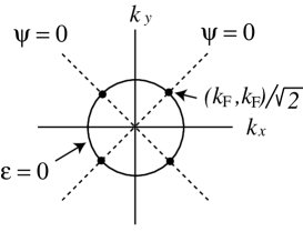
Figure 1: Line nodes in high-$T_{\rm c}$ superconductors.

We will show that the line nodes are stable. We perturb the parameters of the Hamiltonian as

$$\epsilon\rightarrow\epsilon+\delta\epsilon,\quad\psi\rightarrow\psi+\delta\psi,$$

$${\bm{g}}\equiv 0\rightarrow{\bm{g}}=\delta{\bm{g}},\quad{\bm{d}}\equiv 0\rightarrow{\bm{d}}=\delta{\bm{d}}.$$ (47)

First, consider the case of $\delta{\bm{g}}=\delta{\bm{d}}=0$. In this case, the perturbation does not break the parity symmetry. Now Eqs.(41) and (42) reduce to

$$\epsilon({\bm{k}})+\delta\epsilon({\bm{k}})=0,\quad\psi({\bm{k}})+\delta\psi({\bm{k}})=0.$$ (48)

These equations can be satisfied by a small change of the position of the line nodes ${\bm{k}}={\bm{k}}_{0}\rightarrow{\bm{k}}={\bm{k}}_{0}+\delta{\bm{k}}_{0}$. Indeed, expanding Eq.(48) around ${\bm{k}}={\bm{k}}_{0}$, we have

$$\nabla\epsilon({\bm{k}}_{0})\cdot\delta{\bm{k}}_{0}+\delta\epsilon({\bm{k}}_{0})=0,$$

$$\nabla\psi({\bm{k}}_{0})\cdot\delta{\bm{k}}_{0}+\delta\psi({\bm{k}}_{0})=0.$$ (49)

(Here we have used $\epsilon({\bm{k}}_{0})=\psi({\bm{k}}_{0})=0$.) For any $\delta\epsilon$ and $\delta\psi$, there exists $\delta{\bm{k}}_{0}$ which satisfies these equations. Therefore, the perturbation moves the position of the line nodes, but it does not remove the line nodes.

When $\delta{\bm{g}}$ and $\delta{\bm{d}}$ are not zero, Eqs.(41) and (42) become

$$(\epsilon+\delta\epsilon)\cdot(\psi+\delta\psi)=\delta{\bm{g}}\cdot\delta{\bm{d}}.$$ (50)

$$(\epsilon+\delta\epsilon)^{2}-(\psi+\delta\psi)^{2}=\delta{\bm{g}}^{2}-\delta{\bm{d}}^{2},$$ (51)

These two equations give two curves in the $(\psi+\delta\psi,\epsilon+\delta\epsilon)$ plane. As is shown in Fig.2(a), these two curves always have two intersection points near the origin. Therefore, we have two different conditions of line nodes corresponding to the two intersection points. This implies that each line node splits into two after the perturbation as illustrated in Fig.2(b). Although the number of line nodes becomes eight, the line nodes do not vanish by the perturbation.

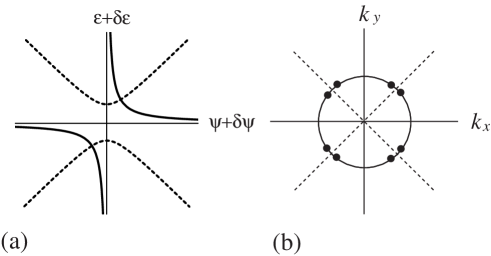
Figure 2: (a) Two curves given by Eqs.(50) (the solid lines) and (51) (the dotted lines). Here we show the case of $\delta{\bm{g}}^{2}-\delta{\bm{d}}^{2}>0$ and $\delta{\bm{g}}\cdot\delta{\bm{d}}>0$. (b) A schematic figure of the line nodes in high-$T_{\rm c}$ superconductors with a parity breaking perturbation.

These line nodes vanish if the time-reversal symmetry is broken. For example, by deforming $\psi({\bm{k}})$ as

$$\psi({\bm{k}})\rightarrow\psi({\bm{k}})+i\eta,\quad(\eta={\rm const.}),$$ (52)

we can completely remove the line nodes.

III.2 polar state in $p$-wave paring

Here we consider the polar state in $p$-wave paring. The polar state is given by

$$\epsilon({\bm{k}})=\frac{{\bm{k}}^{2}}{2m}-\mu,\quad{\bm{d}}({\bm{k}})=\Delta_{0}\hat{{\bm{z}}}k_{z},$$ (53)

and

$$\psi({\bm{k}})={\bm{g}}({\bm{k}})=0.$$ (54)

It is a solution of the Ginzburg-Landau theory neglecting the spin-orbit coupling Leggett (1975). Obviously, the gap has a line node on the equator. See Fig.3.

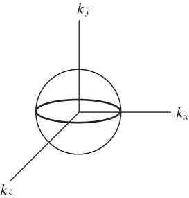
Figure 3: A line node of the polar state in $p$-wave paring.

The line node is unstable, because, for example, the following deformation of the gap function removes the line node completely,

$${\bm{d}}({\bm{k}})\rightarrow{\bm{d}}({\bm{k}})+\eta(\hat{{\bm{x}}}k_{x}+\hat{\bm{y}}k_{z}),$$ (55)

where $\eta$ is a small real number. This line node is not given by an intersection line of Eqs.(41) and (42), thus it is accidental and topologically unstable.

III.3 mixed singlet-triplet states

For noncentrosymmetric materials, the parity symmetry is broken in the normal states. In the presence of the spin-orbit interaction, the absence of inversion symmetry give rise to parity breaking terms ${\bm{g}}({\bm{k}})$ in the normal states. In such systems, singlet and triplet parings can be mixed in the superconducting states Gor’kov and Rashba (2001). We examine stability of line nodes in the mixed singlet-triplet superconducting states.

As a concrete example, consider a $s+p$ superconducting state proposed to explain the superconducting state in ${\rm CePt_{3}Si}$. In this material, the existence of line nodes was reported experimentally Izawa et al. (2005). In ${\rm CePt_{3}Si}$, the absence of inversion symmetry give rise to the Rashba interaction,

$${\bm{g}}({\bm{k}})=\alpha\sqrt{\frac{3}{2}}(-\hat{\bm{x}}k_{y}+\hat{\bm{y}}k_{x}),$$ (56)

where $\alpha$ is a real number. The following gap function was proposed to explain the line node in the superconducting state Hayashi et al. ,

$$\psi({\bm{k}})=\Psi_{0},\quad{\bm{d}}({\bm{k}})=\Delta_{0}(-\hat{\bm{x}}k_{y}+\hat{\bm{y}}k_{x}).$$ (57)

Here $\Psi_{0}$ and $\Delta_{0}$ are real numbers. As is shown in Ref.Hayashi et al. , one can show that under a suitable choice of $\alpha$, $\Psi_{0}$ and $\Delta_{0}$, $E_{-}({\bm{k}})$ has two line nodes. ($E_{+}({\bm{k}})$ has no node.) We show a schematic picture of the nodes in Fig.4. As in the high-$T_{\rm c}$ case, it can be shown that the line nodes are stable against any small time-reversal invariant perturbations; The line nodes are intersection lines of the surfaces given by Eqs.(41) and (42) in momentum space.

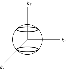
Figure 4: A schematic figure of line nodes on the Fermi surface of ${\rm CePt_{3}Si}$ Hayashi et al. . The sphere and the solid lines denote the Fermi surface and the line nodes, respectively.

Under a small perturbation,

$$\epsilon\rightarrow\epsilon+\delta\epsilon,\quad\psi\rightarrow\psi+\delta\psi,$$

$${\bm{g}}\rightarrow{\bm{g}}+\delta{\bm{g}},\quad{\bm{d}}\rightarrow{\bm{d}}+\delta{\bm{d}},$$ (58)

these surfaces moves slightly, but the intersection lines do not vanish unless the lines shrink to points.

In a similar manner, we can show generally that line nodes are topologically stable in mixed singlet-triplet superconducting states with time-reversal invariance. For example, the line nodes proposed for ${\rm Li_{2}Pd_{3}B}$ and ${\rm Li_{2}Pt_{3}B}$ Yuan et al. are topologically stable.

IV $Z_{2}$ Topological Number

In the previous sections, we have seen that line nodes can be stable in superconducting states with time-reversal invariance. In this section, we show that the stability is explained by the existence of topological numbers defined by wavefunctions of quasiparticles. The topological numbers are closely related to a real structure of the Hamiltonian $H({\bm{k}})$. Although $H({\bm{k}})$ is not a real matrix in general, it has another real structure due to the time-reversal symmetry.

IV.1 Real structure and ${\bm{Z}}_{2}$ topological number

IV.1.1 Real structure

In order to find a real structure, it is convenient to consider the following $8\times 8$ Hamiltonian,

$${\cal H}({\bm{k}})=\left(\begin{array}[]{cc}H({\bm{k}})&0\\ 0&H(-{\bm{k}})\end{array}\right),$$ (61)

and its eigenvalue equation,

$${\cal H}({\bm{k}})\Psi({\bm{k}})=E({\bm{k}})\Psi({\bm{k}}).$$ (62)

The eigenvalue $E({\bm{k}})$ is the same as that of $H({\bm{k}})$.

Using the time-reversal symmetry of $H({\bm{k}})$, we can show

$$\Xi{\cal H}({\bm{k}})\Xi^{-1}={\cal H}({\bm{k}})^{*},$$ (63)

where $\Xi$ is defined by

$$\Xi=\left(\begin{array}[]{cc}0&\Theta\\ -\Theta&0\end{array}\right),\quad\Xi^{2}=1.$$ (66)

The relation (63) implies a real structure of ${\cal H}({\bm{k}})$. To see this, we introduce an operator ${\cal K}=\Xi K$ where $K$ is the ordinary complex-conjugation operator. The new operator obeys ${\cal K}^{2}=1$, then we can think of it as a new complex-conjugation operator. The extended Hamiltonian ${\cal H}({\bm{k}})$ is “real” in terms of the new complex-conjugate operation,

$${\cal K}{\cal H}({\bm{k}}){\cal K}^{-1}={\cal H}({\bm{k}}).$$ (67)

Now we can impose the reality condition on the eigenfunction $\Psi({\bm{k}})$,

$$\Psi({\bm{k}})={\cal K}\Psi({\bm{k}})(\equiv\Xi\Psi({\bm{k}})^{*}).$$ (68)

Using an eigenfunction of $H({\bm{k}})$,

$$H({\bm{k}})u({\bm{k}})=E({\bm{k}})u({\bm{k}}),$$ (69)

we find the following two independent eigenfunctions of ${\cal H}({\bm{k}})$ which satisfy the reality condition,

$$\Psi_{\rm R}({\bm{k}})=\frac{1}{2}\left(\begin{array}[]{c}u({\bm{k}})\\ -\Theta u({\bm{k}})^{*}\end{array}\right),$$ (72)

and

$$\Psi_{\rm I}({\bm{k}})=-\frac{i}{2}\left(\begin{array}[]{c}u({\bm{k}})\\ \Theta u({\bm{k}})^{*}\end{array}\right).$$ (75)

Since $u({\bm{k}})$ is rewritten as

$$\left(\begin{array}[]{c}u({\bm{k}})\\ 0\end{array}\right)=\Psi_{\rm R}({\bm{k}})+i\Psi_{\rm I}({\bm{k}}),$$ (78)

these two wavefunctions correspond to the “real” and “imaginary” parts of $u({\bm{k}})$, respectively. If $u({\bm{k}})$ is normalized as

$$u({\bm{k}})^{\dagger}u({\bm{k}})=1,$$ (79)

the normalization of $\Psi_{A}({\bm{k}})$ is given by

$$\Psi_{A}({\bm{k}})^{\dagger}\Psi_{B}({\bm{k}})=\frac{1}{2}\delta_{AB},$$ (80)

where $A,B={\rm R},{\rm I}$.

IV.1.2 ${\bm{Z}}_{2}$ topological number

To define topological numbers of a line node, let us consider first an infinitesimal circle $S^{1}$ around the line node and solve the eigenequation $H({\bm{k}})u({\bm{k}})=E({\bm{k}})u({\bm{k}})$ on $S^{1}$. (See Fig.5.) Because of the gauge freedom

$$u({\bm{k}})\rightarrow e^{i\theta({\bm{k}})}u({\bm{k}}),$$ (81)

$u({\bm{k}})$ is not determined uniquely. We have to fix the gauge. Generally, a gauge fixed solution has a singularity on $S^{1}$, thus it can not be well-defined on the entire $S^{1}$. Two or more solutions with different gauge fixings are needed to cover the entire $S^{1}$. We consider a couple of solutions $u^{(1)}({\bm{k}})$ and $u^{(2)}({\bm{k}})$, and demand that the first component of $u^{(1)}({\bm{k}})$ and the second one of $u^{(2)}({\bm{k}})$ are real. Because of these different demands, the solutions $u^{(1)}({\bm{k}})$ and $u^{(2)}({\bm{k}})$ have different singularities from each other. Therefore, we can cover the entire $S^{1}$ by using them.

Let us next consider the Kramers doublet of $u^{(2)}({\bm{k}})$, $\Theta u^{(2)}(-{\bm{k}})^{*}$. By definition, the Kramers doublet has the real first component as well as $u^{(1)}({\bm{k}})$. Therefore the following two possibility arises,

1. $\Theta u^{(2)}(-{\bm{k}})^{*}=u^{(1)}({\bm{k}})$ (or $-u^{(1)}({\bm{k}})$),

2. $\Theta u^{(2)}(-{\bm{k}})^{*}\neq\pm u^{(1)}({\bm{k}})$.

Here we concentrate on the latter case, since only this is relevant to the topological numbers of the line node . In this case, $\Theta u^{(2)}(-{\bm{k}})^{*}$ has a different singularity from $u^{(1)}({\bm{k}})$, thus we can use $\Theta u^{(2)}(-{\bm{k}})^{*}$ instead of $u^{(2)}({\bm{k}})$ to cover the entire region of $S^{1}$. After all, the following two solutions with the real first component are obtained,

$$u^{(+)}({\bm{k}})\equiv u^{(1)}({\bm{k}}),\quad u^{(-)}({\bm{k}})\equiv\Theta u^{(2)}(-{\bm{k}})^{*}.$$ (82)

If the solutions $u^{(+)}({\bm{k}})$ and $u^{(-)}({\bm{k}})$ are nonsingular on $U_{+}$ and $U_{-}$, respectively, $S^{1}$ is given by the union of $U_{+}$ and $U_{-}$,

$$S^{1}=U_{+}\cup U_{-}.$$ (83)

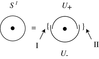
Figure 5: $S^{1}$ around a line node. $S^{1}$ is covered by $U_{+}$ and $U_{-}$. The overlap of $U_{+}$ and $U_{-}$ consists of the regions I and II.

Now it is convenient to introduce the eigenfunctions of ${\cal H}({\bm{k}})$ instead of $u^{(\sigma)}({\bm{k}})$ $(\sigma=\pm)$. The eigenfunctions of ${\cal H}({\bm{k}})$ with the reality condition (68) are constructed from $u^{(\sigma)}({\bm{k}})$ as

$$\Psi^{(\sigma)}_{\rm R}({\bm{k}})=\frac{1}{2}\left(\begin{array}[]{c}u^{(\sigma)}({\bm{k}})\\ -\Theta u^{(\sigma)}({\bm{k}})^{*}\end{array}\right),$$ (86)

$$\Psi^{(\sigma)}_{\rm I}({\bm{k}})=-\frac{i}{2}\left(\begin{array}[]{c}u^{(\sigma)}({\bm{k}})\\ \Theta u^{(\sigma)}({\bm{k}})^{*}\end{array}\right).$$ (89)

It is easily find that the eigenfunctions $\Psi_{A}^{(\sigma)}({\bm{k}})$’s $(A={\rm R},{\rm I})$ are regular in $U_{\sigma}$.

On the overlap $U_{+}\cap U_{-}$, both $\Psi^{(+)}_{A}({\bm{k}})$ and $\Psi^{(-)}_{B}({\bm{k}})$ are regular and they are related by the transition function $T_{AB}({\bm{k}})$,

$$\Psi^{(+)}_{A}({\bm{k}})=T_{AB}({\bm{k}})\Psi^{(-)}_{B}({\bm{k}}).$$ (90)

The reality condition (68) and the normalization (80) imply that the transition function $T({\bm{k}})(\equiv T_{AB}({\bm{k}}))$ is an element of ${\rm O}(2)$. Moreover, $T({\bm{k}})$ reduces to

$$T({\bm{k}})=\left(\begin{array}[]{cc}t_{\rm R}({\bm{k}})&0\\ 0&t_{\rm I}({\bm{k}})\end{array}\right),\quad t_{\rm R}({\bm{k}})=t_{\rm I}({\bm{k}})=\pm 1,$$ (93)

since $\Psi^{(\sigma)}_{\rm R}({\bm{k}})$’s have the real first components but $\Psi^{(\sigma)}_{\rm I}({\bm{k}})$’s have the imaginary ones. Therefore, $\Psi_{\rm R}^{(+)}({\bm{k}})$ (or $\Psi_{\rm I}^{(+)}({\bm{k}})$) is identified with $\Psi_{\rm R}^{(-)}({\bm{k}})$ ($\Psi_{\rm I}^{(-)}({\bm{k}})$) on $U_{+}\cap U_{-}$. As we will show immediately, the transition function determines the global topology of the wavefunctions.

For the sake of simplicity, we assume in the following that both $U_{+}$ and $U_{-}$ are connected regions as illustrated in Fig.5. In this case, the overlap $U_{+}\cap U_{-}$ consists of two regions I and II. The generalization to other cases in which $U_{+}$ and $U_{-}$ consist of many disconnected segments is straightforward.

Let us examine the topology of $\Psi^{(\sigma)}_{\rm R}({\bm{k}})$. On $S^{1}$, it has two transition functions $t_{\rm R}({\bm{k}_{\rm I}})$ and $t_{\rm R}({\bm{k}}_{\rm II})$ where ${\bm{k}}_{\rm I}$ and ${\bm{k}}_{\rm II}$ are arbitrary points on the regions I and II, respectively. If $t_{\rm R}({\bm{k}}_{\rm I})=t_{\rm R}({\bm{k}}_{\rm II})$, $\Psi^{(+)}_{\rm R}({\bm{k}})$ are glued to $\Psi^{(-)}_{\rm R}({\bm{k}})$ without twisting, thus we have a trivial topology similar to a cylinder. (See Fig 6.) This configuration is a contractable loop in the Hilbert space, therefore nothing interesting happens. On the other hand, if $t_{\rm R}({\bm{k}}_{\rm I})=-t_{\rm R}({\bm{k}}_{\rm II})$, $\Psi^{(+)}_{\rm R}({\bm{k}})$ and $\Psi^{(-)}_{\rm R}({\bm{k}})$ are glued together with twisting, thus we have a nontrivial topology similar to the Möbius strip Eguchi et al. (1980). Since this configuration is a noncontractable loop around the line node, the line node can be considered as a kind of topological defect (vortex). Therefore, in this case the line node is stable against a continuous deformation of the Hamiltonian. If we twist the wavefunction in twice, we have a trivial configuration again. Thus, the corresponding homotopy group is $\pi_{1}={\bm{Z}}_{2}$.

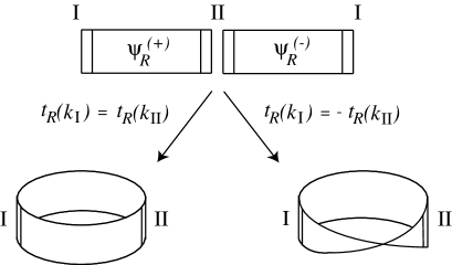
Figure 6: Possible configurations around a line node. (a) A contractable loop. (b) A noncontractable loop.

By this argument, we naturally introduce the following ${\bm{Z}}_{2}$ topological number $I_{\rm R}$,

$$I_{\rm R}=\frac{\ln\left(t_{\rm R}({\bm{k}}_{\rm I})t_{\rm R}({\bm{k}}_{\rm II})\right)}{\pi i}\quad({\rm mod.}2).$$ (94)

It takes

$$I_{\rm R}=\left\{\begin{array}[]{ll}0,&\mbox{for $t_{\rm R}({\bm{k}}_{\rm I})=t_{\rm R}({\bm{k}}_{\rm II})$},\\ 1,&\mbox{for $t_{\rm R}({\bm{k}}_{\rm I})=-t_{\rm R}({\bm{k}}_{\rm II})$}.\end{array}\right.$$ (97)

The line node is topologically stable when $I_{\rm R}=1$ $({\rm mod.}2)$, and the stability is explained by the conservation of the topological number.

In a similar manner, another ${\bm{Z}}_{2}$ topological number can be defined as,

$$I_{\rm I}=\frac{\ln\left(t_{\rm I}({\bm{k}}_{\rm I})t_{\rm I}({\bm{k}}_{\rm II})\right)}{\pi i}\quad({\rm mod.}\,2).$$ (98)

Since $t_{\rm I}({\bm{k}})$ is equal to $t_{\rm R}({\bm{k}})$, it is easily seen that $I_{\rm I}=I_{\rm R}$.

Unless the time-reversal symmetry is broken, the two topological numbers $I_{\rm R}$ and $I_{\rm I}$ are conserved independently. However, once the time-reversal invariance is lost, they are not conserved. The reality of the Hamiltonian (68) is lost and $\Psi_{\rm R}({\bm{k}})$ cannot be distinguished from $\Psi_{\rm I}({\bm{k}})$. Although the summation of $I_{\rm R}$ and $I_{\rm I}$ may be conserved, it is identically zero

$$I_{\rm R}+I_{\rm I}=0\quad({\rm mod.}2).$$ (99)

Therefore, the line node loses the topological stability and it disappears in general.

It can be shown that the topological numbers are gauge invariant if the gauge transformation is nonsingular. Consider the following gauge transformation

$$u({\bm{k}})\rightarrow u^{\prime}({\bm{k}})=e^{i\theta({\bm{k}})}u({\bm{k}}),$$ (100)

where $\theta({\bm{k}})$ is a nonsingular function of ${\bm{k}}$. When $\theta({\bm{k}})$ is nonsingular, the regions $U_{+}$ and $U_{-}$ in which $u^{(+)}{}^{\prime}({\bm{k}})$ and $u^{(-)}{}^{\prime}({\bm{k}})$ are nonsingular remain the same as before. The $U(1)$ gauge transformation (100) induces the following ${\rm SO}(2)$ gauge transformation on $\Psi^{(\sigma)}_{A}({\bm{k}})$,

$$\Psi^{(\sigma)}_{A}{}^{\prime}({\bm{k}})=O_{AB}({\bm{k}})\Psi^{(\sigma)}_{B}({\bm{k}}),$$ (101)

where

$$O({\bm{k}})\equiv O_{AB}({\bm{k}})=\left(\begin{array}[]{cc}\cos\theta({\bm{k}})&-\sin\theta({\bm{k}})\\ \sin\theta({\bm{k}})&\cos\theta({\bm{k}})\end{array}\right).$$ (104)

The new transformation function $T^{\prime}({\bm{k}})$ between $\Psi^{(\sigma)}_{A}{}^{\prime}({\bm{k}})$’s is given by

$$T^{\prime}({\bm{k}})=O({\bm{k}})T({\bm{k}})O({\bm{k}})^{\rm T}.$$ (105)

Because the ${\rm O}(2)$ matrices $O({\bm{k}})$ and $T({\bm{k}})$ commute with each other, we obtain

$$T^{\prime}({\bm{k}})=T({\bm{k}}).$$ (106)

Therefore, the topological numbers $I_{\rm R}$ and $I_{\rm I}$ defined by $T({\bm{k}})$ are gauge invariant.

IV.2 high-${\rm T_{c}}$ materials

The Hamiltonian of high-$T_{\rm c}$ superconductors is

$$H({\bm{k}})=\left(\begin{array}[]{cc}\epsilon({\bm{k}})&i\psi({\bm{k}})\sigma_{2}\\ -i\psi({\bm{k}})\sigma_{2}&-\epsilon({\bm{k}})\end{array}\right).$$ (109)

This superconducting state is unitary, thus the quasiparticle energies $E_{\pm}({\bm{k}})$ are degenerate in the entire momentum space,

$$E_{\pm}({\bm{k}})=E({\bm{k}})=\sqrt{\epsilon({\bm{k}})^{2}+\psi({\bm{k}})^{2}}.$$ (110)

Since the parity is conserved and $H({\bm{k}})$ is real, $H({\bm{k}})$ commutates with $\Theta$,

$$\Theta H({\bm{k}})=H({\bm{k}})\Theta.$$ (111)

Therefore, the eigenfunctions $u_{i}({\bm{k}})$ ($i=1,2$) with $E({\bm{k}})$ can be the eigenfunction of $\Theta$ simultaneously,

$$\Theta u_{1}({\bm{k}})=iu_{1}({\bm{k}}),\quad\Theta u_{2}({\bm{k}})=-iu_{2}({\bm{k}}).$$ (112)

Consider a line node shown in Fig.7.

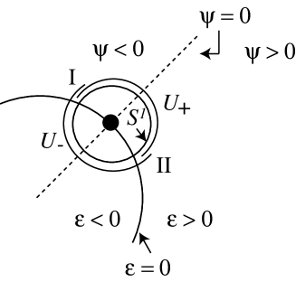
Figure 7: $S^{1}$ around a line node in high-$T_{\rm c}$ superconductors

The eigenfunctions regular in $U_{+}$ are given by

$$u_{1}^{(+)}({\bm{k}})=\frac{1}{2\sqrt{E(E+\epsilon)}}\left(\begin{array}[]{c}(E+\epsilon)\\ i(E+\epsilon)\\ -i\psi\\ \psi\end{array}\right),$$ (117)

$$u_{2}^{(+)}({\bm{k}})=\frac{1}{2\sqrt{E(E+\epsilon)}}\left(\begin{array}[]{c}E+\epsilon\\ -i(E+\epsilon)\\ i\psi\\ \psi\end{array}\right),$$ (122)

and those regular in $U_{-}$ are

$$u_{1}^{(-)}({\bm{k}})=\frac{1}{2\sqrt{E(E-\epsilon)}}\left(\begin{array}[]{c}\psi\\ i\psi\\ -i(E-\epsilon)\\ E-\epsilon\end{array}\right),$$ (127)

$$u_{2}^{(-)}({\bm{k}})=\frac{1}{2\sqrt{E(E-\epsilon)}}\left(\begin{array}[]{c}\psi\\ -i\psi\\ i(E-\epsilon)\\ E-\epsilon\end{array}\right).$$ (132)

In a similar manner as $t_{A}({\bm{k}})$ and $I_{\rm A}$ $(A={\rm R},{\rm I})$ in the previous subsection, the transition functions $t_{aA}({\bm{k}})$ and the topological number $I_{aA}$ $(a=1,2,\,A={\rm R},{\rm I})$ are constructed from $u_{a}^{(\sigma)}({\bm{k}})$ $(a=1,2,\,\sigma=\pm)$. The transition functions become

$$t_{1{\rm R}}({\bm{k}})=t_{1{\rm I}}({\bm{k}})={\rm sgn}\psi({\bm{k}}),$$

$$t_{2{\rm R}}({\bm{k}})=t_{2{\rm I}}({\bm{k}})={\rm sgn}\psi({\bm{k}}).$$ (133)

Because the transition functions have different signatures between regions I and II in Fig.7, the topological numbers calculated on $S^{1}$ are given by

$$I_{1{\rm R}}=I_{1{\rm I}}=1,\quad I_{2{\rm R}}=I_{2{\rm I}}=1.$$ (134)

As long as the parity is conserved, the eigenfunctions of $H({\bm{k}})$ stay the eigenfunctions of $\Theta$. Therefore, $I_{1A}$ and $I_{2A}$ $(A={\rm R},{\rm I})$ are not mixed, and the stability of the line node is ensured by conservation of these topological numbers.

If the parity is broken, the degeneracy between $E_{+}({\bm{k}})$ and $E_{-}({\bm{k}})$ is resolved and only $E_{-}({\bm{k}})$ has line nodes. When the perturbation is small enough, the topological numbers $I_{\rm R}$ and $I_{\rm I}$ defined by the eigenfunction with $E_{-}({\bm{k}})$ are calculated on the same $S^{1}$ as

$$I_{\rm R}=I_{1{\rm R}}+I_{2{\rm R}}=0,\quad I_{\rm I}=I_{1{\rm I}}+I_{2{\rm I}}=0.$$ (135)

This is consistent with the splitting of the line nodes shown in Sec.III.1; The line node in Fig.7 is divided into two as is shown in Sec.III.1, and each divided line node has the topological numbers $I_{\rm R}=I_{\rm I}=1$. Because $S^{1}$ encloses both the divided line nodes, the topological numbers calculated on $S^{1}$ become $I_{\rm R}=I_{\rm I}=1+1=0$ which is the same as Eq.(135).

IV.3 polar state in $p$-wave paring

The Hamiltonian of the polar state in $p$-wave paring is

$$H({\bm{k}})=\left(\begin{array}[]{cc}\epsilon({\bm{k}})&d_{3}({\bm{k}})\sigma_{1}\\ d_{3}({\bm{k}})\sigma_{1}&-\epsilon({\bm{k}})\end{array}\right).$$ (138)

The quasiparticle energies $E_{\pm}({\bm{k}})=E({\bm{k}})$ are given by

$$E({\bm{k}})=\sqrt{\epsilon({\bm{k}})^{2}+d_{3}({\bm{k}})^{2}}.$$ (139)

Consider a circle $S^{1}$ around the line node in the equator. (See Fig.8.)

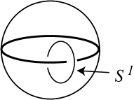
Figure 8: $S^{1}$ around the line node in the polar state.

The circle $S^{1}$ is covered by the following solutions,

$$u_{1}^{(+)}({\bm{k}})=\frac{1}{2\sqrt{E(E+\epsilon)}}\left(\begin{array}[]{c}E+\epsilon\\ E+\epsilon\\ d_{3}\\ d_{3}\end{array}\right),$$ (144)

$$u_{1}^{(-)}({\bm{k}})=\frac{1}{2\sqrt{E(E-\epsilon)}}\left(\begin{array}[]{c}d_{3}\\ d_{3}\\ E-\epsilon\\ E-\epsilon\end{array}\right),$$ (149)

$$u_{2}^{(+)}({\bm{k}})=\frac{1}{2\sqrt{E(E+\epsilon)}}\left(\begin{array}[]{c}E+\epsilon\\ -(E+\epsilon)\\ -d_{3}\\ d_{3}\end{array}\right),$$ (154)

$$u_{2}^{(-)}({\bm{k}})=\frac{1}{2\sqrt{E(E-\epsilon)}}\left(\begin{array}[]{c}-d_{3}\\ d_{3}\\ E-\epsilon\\ -(E-\epsilon)\end{array}\right).$$ (159)

Using these solutions, we obtain the transition functions as follows,

$$t_{1{\rm R}}({\bm{k}})=t_{1{\rm I}}({\bm{k}})={\rm sgn}d_{3}({\bm{k}}),$$

$$t_{2{\rm R}}({\bm{k}})=t_{2{\rm I}}({\bm{k}})=-{\rm sgn}d_{3}({\bm{k}}).$$ (160)

From this, the topological numbers are calculated as

$$I_{1{\rm R}}=I_{1{\rm I}}=1,\quad I_{1{\rm R}}=I_{1{\rm I}}=1.$$ (161)

At a first glass, it seems to suggest that the line node has nontrivial topological numbers. However, on the contrary to the high-$T_{\rm c}$ case, there is no quantum number which distinguishes $u_{1}^{(\sigma)}({\bm{k}})$ from $u_{2}^{(\sigma)}({\bm{k}})$ $(\sigma=\pm)$. Therefore, only the summations $I_{1A}+I_{2A}=0$ $(A={\rm R},{\rm I})$ are preserved, and the line node has no nontrivial topological numbers. This result is consistent with the result in Sec.III.2; The line node is unstable against a small perturbation of $H({\bm{k}})$.

IV.4 mixed singlet-triplet state

The Hamiltonian of mixed singlet-triplet states is

$$H({\bm{k}})=\left(\begin{array}[]{cc}\epsilon({\bm{k}})+{\bm{g}}({\bm{k}})\cdot{\bm{\sigma}}&\Delta({\bm{k}})\\ \Delta({\bm{k}})^{\dagger}&-\epsilon({\bm{k}})+{\bm{g}}({\bm{k}})\cdot{\bm{\sigma}}^{*}\end{array}\right),$$ (164)

where

$$\Delta({\bm{k}})=i\psi({\bm{k}})\sigma_{2}+i{\bm{d}}({\bm{k}})\cdot{\bm{\sigma}}\sigma_{2}.$$ (165)

Here $\psi({\bm{k}})$ and ${\bm{d}}({\bm{k}})$ are real functions. As was shown in Ref.Frigeri et al. (2004), ${\bm{d}}({\bm{k}})$ is proportional to ${\bm{g}}({\bm{k}})$ in mixed singlet-triplet states,

$${\bm{d}}({\bm{k}})=c{\bm{g}}({\bm{k}}).$$ (166)

For the sake of simplicity, we assume $c>0$ in the following. $E_{-}({\bm{k}})$ is given by

$$E_{-}({\bm{k}})$$

$$= \sqrt{(\epsilon({\bm{k}})-{\rm sgn}\psi({\bm{k}})|{\bm{g}}({\bm{k}})|)^{2}+(|\psi({\bm{k}})|-|{\bm{d}}({\bm{k}})|)^{2}}.$$

The eigenfunction has the following two forms,

$$u^{(+)}({\bm{k}}) = \frac{1}{\sqrt{2E_{-}(E_{-}+\epsilon-{\rm sgn}\psi|{\bm{g}}|)}}$$ (170)

$$\times \left(\begin{array}[]{c}\left(E_{-}+\epsilon-{\rm sgn}\psi|{\bm{g}}|\right)\phi\\ -i{\rm sgn}\psi\left(|\psi|-|{\bm{d}}|\right)\sigma_{2}\phi\end{array}\right),$$

$$u^{(-)}({\bm{k}}) = \frac{1}{\sqrt{2E_{-}(E_{-}-\epsilon+{\rm sgn}\psi|{\bm{g}}|)}}$$ (173)

$$\times \left(\begin{array}[]{c}{\rm sgn}\psi\left(|\psi|-|{\bm{d}}|\right)\phi\\ -i\left(E_{-}-\epsilon+{\rm sgn}\psi|{\bm{g}}|\right)\sigma_{2}\phi\end{array}\right),$$

where $\phi({\bm{k}})$ satisfies

$${\bm{d}}({\bm{k}})\cdot{\bm{\sigma}}\phi({\bm{k}})=-{\rm sgn}\psi({\bm{k}})|{\bm{d}}({\bm{k}})|\phi({\bm{k}}).$$ (174)

The first components of $u^{(\pm)}({\bm{k}})$ are real if we choose

$$\phi({\bm{k}})=$$

$$\left\{\begin{array}[]{cc}\frac{1}{\sqrt{2|{\bm{d}}|(|{\bm{d}}|-d_{3})}}\left(\begin{array}[]{c}|{\bm{d}}|-d_{3}\\ -d_{1}-id_{2}\end{array}\right),&(\mbox{for ${\rm sgn}\psi>0$})\\ \frac{1}{\sqrt{2|{\bm{d}}|(|{\bm{d}}|+d_{3})}}\left(\begin{array}[]{c}|{\bm{d}}|+d_{3}\\ d_{1}+id_{2}\end{array}\right),&(\mbox{for ${\rm sgn}\psi<0$})\end{array}\right..$$ (181)

The transition functions obtained from $u^{(+)}({\bm{k}})$ and $u^{(-)}({\bm{k}})$ are

$$t_{\rm R}({\bm{k}})=t_{\rm I}({\bm{k}})={\rm sgn}\psi({\bm{k}})\cdot{\rm sgn}(|\psi({\bm{k}})|-|{\bm{d}}({\bm{k}})|).$$ (183)

From these transition functions, we can calculate the topological numbers $I_{\rm R}$ and $I_{\rm I}$ of line nodes in mixed singlet-triplet superconducting states. For example, the straightforward calculation shows that both the line nodes of ${\rm CeSi_{3}Pt}$ in Fig.4 have nontrivial topological numbers, $I_{\rm R}=I_{\rm I}=1$. We can also show that the line nodes proposed for ${\rm Li_{2}Pd_{3}B}$ and ${\rm Li_{2}Pt_{3}B}$ Yuan et al. have nontrivial topological numbers. These results are consistent with the stability of the line nodes examined in Sec.III.3.

Note that the time-reversal symmetry is essential for the stability of the line nodes. For example, when $\psi({\bm{k}})$ becomes complex, the time-reversal symmetry is broken. In this case, the quasiparticle spectra are given by

$$E({\bm{k}})$$

$$= \pm\sqrt{\left(\epsilon({\bm{k}})\pm|{\bm{g}}({\bm{k}})|\right)^{2}+\left({\rm Re}\psi({\bm{k}})\pm|{\bm{d}}({\bm{k}})|\right)^{2}+\left({\rm Im}\psi({\bm{k}})\right)^{2}}.$$

If ${\rm Im}\psi({\bm{k}})$ is a nonzero constant, the line nodes in the mixed singlet-triplet states vanish completely.

V Conclusions and Discussions

(1) First we would like to outline the results of this paper. We examined topological stability of line nodes in superconducting states with time-reversal invariance. A generic Hamiltonian of time-reversal invariant superconducting states was presented. We found that only line nodes are topologically stable in single-band descriptions of superconductivity. It was shown that line nodes in high-$T_{\rm c}$ materials and mixed singlet-triplet superconducting states are topologically stable, while one in the polar state is not. Using the time-reversal symmetry, we introduced a real structure and defined ${\bm{Z}}_{2}$ topological numbers. Stability of line nodes was explained by conservation of the topological numbers.

(2) Besides the superconducting states examined in this paper, several superconductors such as ${\rm CeCoIn}_{5}$ Tanatar et al. (2005), ${\rm CeIrIn}_{5}$ Movshovich et al. (2001) and ${\rm Sr_{2}RuO_{4}}$ Suzuki et al. (2002); Izawa et al. (2001a); Deguchi et al. (2004a, b) are believed to host line nodes. Among them, the gap function of ${\rm CeCoIn}_{5}$ is a $d$-wave paring, thus its line nodes are topologically stable in a similar manner as high-$T_{\rm c}$ materials. On the other hand, the line nodes of ${\rm Sr_{2}RuO_{4}}$ are not topologically stable since its superconducting state breaks the time-reversal symmetry Luke et al. (1998).

(3) An analysis based on the KR theory Hořava (2005) shows that point nodes have a ${\bm{Z}}_{2}$ topological number in a nonrelativistic Fermi system with the time-reversal symmetry. However, our analysis in Sec.II indicates that point nodes have only the trivial topological number if the superconducting state is described by single-band electrons.

(4) If the superconductivity occurs in multi-bands of electrons, a topologically stable point node is possible to exist. In other words, if the time-reversal symmetry is not broken, the existence of a topological stable point node implies a multi-band superconductivity.

(5) For mixed singlet-triplet superconducting states, the existence of the line nodes is not explained by the group theoretical method in Refs.Volovik and Gor’kov (1984, 1985); Blount (1985); Ueda and Rice (1985, ). The topological stability studied here is essential for the existence of these line nodes.

(6) In addition to the time-reversal symmetry, if the party is conserved, the Hamiltonian becomes

$$H({\bm{k}})=\left(\begin{array}[]{cc}\epsilon({\bm{k}})&i\psi({\bm{k}})\sigma_{2}\\ -i\psi({\bm{k}})\sigma_{2}&-\epsilon({\bm{k}})\end{array}\right).$$ (187)

This is a real symmetric matrix, thus we have a natural real structure. Using this real structure, we can introduce a ${\bm{Z}}_{2}$ topological number which is different from that given in Sec.IV as follows Sato (2004). Let us consider the eigenfunction of $H({\bm{k}})u({\bm{k}})=E({\bm{k}})u({\bm{k}})$,

$$u({\bm{k}})=\left(\begin{array}[]{c}a({\bm{k}})\\ b({\bm{k}})\\ c({\bm{k}})\\ d({\bm{k}})\end{array}\right),$$ (192)

Here we can demand $a({\bm{k}})$, $b({\bm{k}})$, $c({\bm{k}})$ and $b({\bm{k}})$ to be real since $H({\bm{k}})$ is a real matrix. If we impose the normalization condition on $u({\bm{k}})$, we have $a({\bm{k}})^{2}+b({\bm{k}})^{2}+c({\bm{k}})^{2}+d({\bm{k}})^{2}=1$, and by using the gauge freedom of the eigenequation, $u({\bm{k}})$ can be identified with $-u({\bm{k}})$. Therefore, $u({\bm{k}})$ is given by an element of $S^{3}/{\bm{Z}}_{2}$ .

Now consider a map determined by $u({\bm{k}})$ from an infinitesimal $S^{1}$ around a line node into $S^{3}/{\bm{Z}}_{2}$. The map is classified by $\pi_{1}(S^{3}/{\bm{Z}}_{2})$. Using the homotopy theory Schwarz (1991), we obtain

$$\pi_{1}(S^{3}/{\bm{Z}}_{2})=\pi_{0}({\bm{Z}}_{2})={\bm{Z}}_{2}.$$ (193)

Therefore, we have a ${\bm{Z}}_{2}$ topological number corresponding to $\pi_{1}(S^{3}/{\bm{Z}}_{2})$. The line node is topologically stable if the map corresponds to the nontrivial element of ${\bm{Z}}_{2}$. A straightforward calculation shows that the map around a line node in high-$T_{\rm c}$ materials gives the nontrivial element. This is another explanation of topological stability of the line nodes in high-$T_{\rm c}$ materials.

Although the construction of this topological number is easier than that given in Sec.IV, it is available only when the parity is conserved.

(7) We have noticed that when a line node splits in two as was shown in Sec.III.1, there remains a degenerate point between $E_{+}({\bm{k}})$ and $E_{+}({\bm{k}})$ near the line node. The degenerate point is topologically stable since it is given by an intersection point of the three equations $\epsilon({\bm{k}}){\bm{g}}({\bm{k}})+\psi({\bm{k}}){\bm{d}}({\bm{k}})=0$ in three dimensional momentum space. The degenerate point has a topological number similar to that of the chiral fermion in Ref.Nilesen and Ninomiya (1981). In order to describe the splitting of the line node in terms of the topological numbers given in this paper, we need to take into account the conservation law of this also.

Note added.- After completing this work, the author noticed a preprint Volovik by G. E. Volovik in which the topological stability of line nodes in high-$T_{\rm c}$ superconductors was discussed very recently. There is some overlap between his paper and Sec.IV.2 in this paper. His argument was restricted to the case where the Hamiltonian is real, while the argument described here is not restricted.