How does a protein search for the specific site on DNA: the role of disorder

Abstract

Proteins can locate their specific targets on DNA up to two orders of magnitude faster than the Smoluchowski three-dimensional diffusion rate. This happens due to non-specific adsorption of proteins to DNA and subsequent one-dimensional sliding along DNA. We call such one-dimensional route towards the target ”antenna”. We studied the role of the dispersion of nonspecific binding energies within the antenna due to quasi random sequence of natural DNA. Random energy profile for sliding proteins slows the searching rate for the target. We show that this slowdown is different for the macroscopic and mesoscopic antennas.

A protein binding to a specific site on DNA, which we call the target, is one of the central paradigms of biology Gann . Well known examples include lac-repressor in E. coli, which regulates a specific gene producing enzyme consuming lactose and the proper restriction enzyme destroying genome of invading E. coli $\lambda$-phage in real time warfare for bacteria survival. It is known since the early days of molecular biology that in some cases proteins can find their target sites along a DNA chain one to two orders faster than the maximum rate achievable by three-dimensional diffusion Riggs ; Richter . To resolve this paradox, nonspecific binding and subsequent one-dimensional sliding of proteins along the DNA to the target was suggested as an important component of the searching process Riggs ; Richter . This idea was studied in various models proposed by both physicists and biologists BWH ; Bruinsma ; Marko ; Halford ; Klenin . A comprehensive study of interplay between the 1D sliding and 3D diffusion for different DNA conformations on the search rate can be found in Ref. Firstpaper .

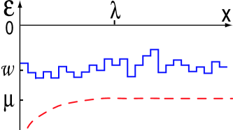
Figure 1: Distribution of nonspecific adsorption energies $\epsilon$ and of chemical potential $\mu(x)$ along DNA molecule. The target site is located at $x=0$, $\lambda$ is the antenna length.

Some authors calculate the typical time $\tau$ needed for the target site to be found by a protein, when a small concentration $c$ of proteins is randomly introduced into the system. Other authors Firstpaper consider the specific site as a sink consuming proteins with the diffusion limited rate $J$ proportional to the concentration $c$ (which in turn should be supported on a constant level by an influx of proteins into the system). Obviously then, $\tau=1/J$. Search rate enhancement due to the sliding along DNA may be calculated as the ratio of the rate $J$ to the 3D Smoluchowski rate $J_{s}=4\pi D_{3}cb$ of diffusion to the sphere of radius $b$ modeling the target site on DNA. The central physical idea is that one can define a piece of DNA adjacent to the target for which 1D sliding diffusion dominates over parallel 3D diffusion channel and which, therefore, serves as a receiving antenna for the 3D Smoluchowski-like diffusion of proteins. Then the key point of the theory is to find the antenna length $\lambda$. In the language of stationary flux $J$, this is done by matching incoming 3D flux $J_{3}$ of proteins to the antenna with the 1D flux $J_{1}$ of proteins sliding on the antenna toward the target.

All the cited above works assume that the nonspecific adsorption energy $w$ of protein is sequence independent, i.e. the energy profile experienced by the searching protein away from the target is totally flat. This however disagrees with quasi-random character of the natural sequences of DNA. It is known that the nonspecific protein-DNA adsorption energy can be divided into two parts BH ; Gerland : (i) The sequence independent Coulomb energy of attraction between the positively charged domain of the protein surface and the negatively charged phosphate backbone, and (ii) the sequence specific adsorption energy due to formation of hydrogen bonds of the protein with the DNA bases. This is done by the recognition $\alpha$-helix going deep into the major groove of DNA Gann . Suppose the protein encounters $l$ base pairs between positions $i$ and $i+l$. We call this position of the protein site i and characterize it by energy $\epsilon_{i}<0$, where the energy of the free protein in water is chosen to be 0. Because the sliding protein has a complex nonuniform structure and interacts with a random DNA sequence, the total energy $\epsilon_{i}$ randomly fluctuates along DNA (Fig. 1). One can assume that at nonspecific positions on DNA, the protein exploits the same set of potential hydrogen bonds it forms with the target Barbi . Since target recognition is often mediated by hydrogen bonds to some of the four chemical groups on the major groove side of the base pair Nadassy , and the recognition $\alpha$-helix interacts with several base pairs, many hydrogen bonds contribute to $\epsilon_{i}$. Therefore the distribution of $\epsilon_{i}$ can be approximated by the Gaussian distribution Barbi ; Mirny ; Kardar with a mean $w$ and standard deviation $\sigma\ll|w|$:

$$g(\epsilon_{i})=\frac{1}{\sqrt{2\pi\sigma^{2}}}\exp\left[-\frac{(\epsilon_{i}-w)^{2}}{2\sigma^{2}}\right].$$ (1)

In this paper we study a role of disorder on the rate enhancement $J/J_{s}$ assuming that disorder is strong, i.e. $\sigma>kT$, where $k$ is the Boltzmann constant and $T$ is the ambient temperature.

Similar to the the case of the flat energy profile Firstpaper , we assume that transport outside the antenna is mainly due to the 3D diffusion, while inside the antenna transport is dominated by sliding, or 1D diffusion along DNA and we equate the fluxes $J_{1}$ and $J_{3}$ to find $\lambda$. The rate $J_{3}$ is given by the Smoluchowski formula for the target size $\lambda$ and for the concentration of “free” (not adsorbed) proteins $c_{3}$, it is $J_{3}\sim D_{3}c_{3}\lambda$. The flux on antenna $J_{1}$ strongly depends on $\sigma$ and also, generally speaking, on DNA sequence in the finite antenna. We show that there is a characteristic length of antenna $\lambda=\lambda_{c}(\sigma,T)$ such that at $\lambda>\lambda_{c}$ flux $J_{1}$ self-averages and becomes sequence independent. Such a ”macroscopic” antenna determines $J/J_{s}$ for moderate disorder. In this case, the ratio $J/J_{s}$ decreases exponentially fast with growth of disorder. At stronger disorder we deal with a mesoscopic antenna with $\lambda<\lambda_{c}$ and strictly speaking $J/J_{s}$ depends on random DNA sequence. In this paper, we concentrate only on the most probable value of $J/J_{s}$. In order to calculate it, we estimate the most probable value of $J_{1}$. We show that in such a mesoscopic situation disorder leads to a weaker reduction of $J/J_{s}$.

We assume that within some volume $v$ there is a straight, immobile (double helical) DNA with the length $L$ smaller than $v^{1/3}$, but much larger than any antenna length. For a dilute DNA solution, $1/v$ stands for the concentration of DNA. We also assume that all the microscopic length scales such as the length of a base pair, the size of the target site, the diameter of the DNA etc. are of the same order $b$. We are mainly interested in scaling dependence of the rate enhancement $J/J_{s}$ on major system parameters, such as $\sigma$, $w$, $L$ and $v$. This means that all the numerical coefficients are dropped in our scaling estimates.

To estimate $J_{1}$, we assume at each site $i$ on DNA, the protein has some probabilities of hopping to nearest neighboring sites $j$. We write the probability for the hopping from an occupied site $i$ to an empty site $j$ as

$$\gamma_{ij} = \nu_{0}\exp\left(-\frac{\epsilon_{j}-\epsilon_{i}+|\epsilon_{j}-\epsilon_{i}|}{2kT}\right)$$ (4)

$$= \left\{\begin{array}[]{lcr}\nu_{0}\exp(-\frac{\epsilon_{j}-\epsilon_{i}}{kT})&{\rm if}&\epsilon_{j}>\epsilon_{i}\\ \nu_{0}&{\rm if}&\epsilon_{j}<\epsilon_{i}\end{array}\right.,\$$

where $\nu_{0}\sim D_{1}/b^{2}$ is the effective attempt frequency. In Eq. (4) we neglected the activation barriers separating two states in comparison with $\epsilon_{j}-\epsilon_{i}$. The number of proteins making such transition from site $i$ to $j$ per unit time can be estimated by $\Gamma_{ij}=\gamma_{ij}f_{i}(1-f_{j})$, where function $f_{i}$ is the average occupation number of site $i$. At small enough $c$, all $f_{i}\ll 1$ and thus $\Gamma_{ij}\simeq\gamma_{ij}f_{i}$. Function $f_{i}$ is given then by:

$$f_{i}=\exp[-(\epsilon_{i}-\mu_{i})/kT],$$ (5)

where $\mu_{i}$ is the chemical potential. Using $\Gamma_{ij}$ and $\Gamma_{ji}$, we can write the net flux from site $i$ to $j$ in the form:

$$J_{ij}=\Gamma_{ij}-\Gamma_{ji}\simeq\nu_{0}e^{-\frac{\epsilon_{ij}}{kT}}(e^{\frac{\mu_{i}}{kT}}-e^{\frac{\mu_{j}}{kT}}),$$ (6)

where $\epsilon_{ij}=max\{\epsilon_{i},\epsilon_{j}\}$.

We now argue that as long as the antenna is only a small part of the DNA molecule, every protein adsorbs to DNA and desorbs many times before it locates the target. Therefore, outside the antenna there is statistical equilibrium between adsorbed and desorbed proteins, and hence proteins have uniform chemical potential $\mu_{i}=\mu=kT\ln(c_{3}b^{3})$. Within the antenna, $\mu_{i}$ decreases when the site approaches the target and reaches $-\infty$ at the target site (see Fig. 1). If we label the border of the antenna as site $1$ and the target as site $\lambda/b+1$, using Eq. (6), we can write

$$\sum_{i=1}^{\lambda/b}J_{ij}e^{\frac{\epsilon_{ij}}{kT}}=\nu_{0}(e^{\frac{\mu}{kT}}-e^{-\frac{\infty}{kT}})=\nu_{0}c_{3}b^{3},$$ (7)

where $j=i+1$. Since the 1D current $J_{1}$ towards the target is the same at any antenna site, i. e. $J_{ij}=J_{1}$, we can find it as

$$J_{1}=\frac{\nu_{0}c_{3}b^{3}}{\sum_{i=1}^{\lambda/b}\exp(\epsilon_{ij}/kT)}\simeq\frac{\nu_{0}c_{3}b^{3}\sqrt{2\pi\sigma^{2}}}{(\lambda/b)\int_{-\infty}^{0}d\epsilon_{ij}R(\epsilon_{ij})},$$ (8)

where $R(\epsilon_{ij})$ is given by

$$R(\epsilon_{ij}) = \sqrt{2\pi\sigma^{2}}g(\epsilon_{ij})\exp(\epsilon_{ij}/kT)$$

$$= \exp\left\{\frac{\sigma^{2}}{2(kT)^{2}}+\frac{w}{kT}-\frac{[\epsilon_{ij}-(w+\sigma^{2}/kT)]^{2}}{2\sigma^{2}}\right\}.$$

One can interpret Eq. (8) as the Ohm’s law, where the numerator plays the role of the voltage applied to antenna and denominator is the sum of resistances of all pairs $(i,j)$ which are similar to Miller-Abrahams resistances for the hopping transport of electrons ES .

The sharp maximum value of function $R(\epsilon_{ij})$ determining the sum of Eq. (8) is reached when $\epsilon_{ij}=\epsilon_{opt}=w+\sigma^{2}/kT$, and $R(\epsilon_{opt})\sim\exp[\sigma^{2}/2(kT)^{2}+w/kT]$. Thus

$$J_{1}\sim\frac{D_{3}c_{3}b^{2}}{\lambda}\exp\left[\frac{|w|}{kT}-\frac{\sigma^{2}}{2(kT)^{2}}\right],$$ (10)

where we assumed for simplicity that $D_{3}=D_{1}\sim b^{2}\nu_{0}$.

Before we move forward, we emphasize the crucial assumption already made in above derivation. We assumed $\lambda$ is so long that within the antenna the sliding protein encounters sites with energy $\epsilon_{opt}$ more than once and therefore, the sum in Eq. (8) can be replaced by the integral with limits from $-\infty$ to $0$. We call such antenna macroscopic. For a short antenna, the probability for such a site to appear inside is very small. Thus the sum in Eq. (8) is determined by the largest value of $R(\epsilon_{ij})$ typically available within the antenna. We call such antenna mesoscopic.

Macroscopic antenna—We study macroscopic antenna first. Using $J_{1}$ and $J_{3}$, our main balance equation for the rate $J$ reads

$$J\sim D_{3}c_{3}\lambda\sim\frac{D_{3}c_{3}b^{2}}{\lambda}\exp\left[\frac{|w|}{kT}-\frac{\sigma^{2}}{2(kT)^{2}}\right]\ .$$ (11)

Thus the antenna length $\lambda$ is obtained as

$$\lambda\sim b\exp\left[\frac{|w|}{2kT}-\frac{\sigma^{2}}{4(kT)^{2}}\right].$$ (12)

Next we calculate the free protein concentration $c_{3}$. Suppose the one-dimensional concentration of non-specifically adsorbed proteins is $c_{1}$. Assuming the antenna is only a small part of the DNA and remembering that adsorbed proteins are confined within distance of order $b$ from the DNA, we can write down the equilibrium condition as:

$$\frac{c_{1}}{c_{3}b^{2}}\sim\int f(\epsilon)e^{-\epsilon/kT}d\epsilon\sim\exp\left[\frac{|w|}{kT}+\frac{\sigma^{2}}{2(kT)^{2}}\right],$$ (13)

which must be complemented by the particle counting condition $c_{1}L+c_{3}(v-Lb^{2})=cv$. Since volume fraction of DNA is always small, $Lb^{2}\ll v$, standard algebra then yields

$$c_{3} \simeq \frac{cv}{yLb^{2}+v}\sim\left\{\begin{array}[]{lcr}c&{\rm if}&y<v/Lb^{2}\\ cv/Lb^{2}y&{\rm if}&y>v/Lb^{2}\end{array}\right.,$$ (16)

where $y$ is $\exp[|w|/kT+\sigma^{2}/2(kT)^{2}]$. Eqs. (16) lead to two different scaling regimes, which are denoted as A and B in the diagram Fig. 2. In regime A, the non-specific adsorption is relatively weak, $c_{3}\sim c$, we arrive at

$$\frac{J}{J_{s}}\sim\exp\left[\frac{|w|}{2kT}-\frac{\sigma^{2}}{4(kT)^{2}}\right].\ \ \ \ \ ({\rm regime\ A})$$ (17)

In the regime B, most proteins are adsorbed. Using the lower line of Eqs. (16), we obtain

$$\frac{J}{J_{s}}\sim\frac{v}{Lb^{2}}\exp\left[-\frac{|w|}{2kT}-\frac{3\sigma^{2}}{4(kT)^{2}}\right].\ \ \ \ \ ({\rm regime\ B})$$ (18)

In both regimes, $|w|>\sigma^{2}/kT$, thus $\sigma$ term of $\ln(J/J_{s})$ constitutes a correction. The size of antenna grows with $|w|$, however unproductive non-specific adsorption of proteins on distant pieces of DNA, which can slow down the transport to the specific target grows with $|w|$ too. These two effects compete, as a result the rate enhancement $J/J_{s}$ grows with $w$ in regime A and declines in regime B. On the other hand, growing $\sigma$ reduces the antenna size and promotes non-specific adsorption. Therefore, $J/J_{s}$ decreases with $\sigma$ in both regimes.

The above theory deals with a macroscopic antenna. To be macroscopic, the antenna has to contain at least one site with energy around $\epsilon_{opt}$. The number of sites $n(\epsilon)$ with energy $\epsilon$ within the antenna is of the order of $\sim(\lambda/b)\exp[-(\epsilon-w)^{2}/2\sigma^{2}]$. Thus a macroscopic antenna requires $n(\epsilon_{opt})>1$, which gives $\lambda>\lambda_{c}=b\exp[\sigma^{2}/2(kT)^{2}]$. Since we know $\lambda$ from Eq. (12), this condition can be written explicitly as $|w|>3\sigma^{2}/2kT$. Hence, $|w|=3\sigma^{2}/2kT$ is the border between the macroscopic regimes (A, B) and mesoscopic regimes (C, D) in Fig. 2. We can check that when $|w|>3\sigma^{2}/2kT$, the condition $\epsilon_{opt}<0$ is satisfied for the case of macroscopic antenna. Now we are ready to switch to the case of mesoscopic antenna and explain regimes C and D.

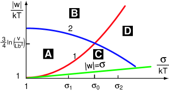
Figure 2: (color online) The phase diagram of scaling regimes for $|w|>\sigma>kT$. Each line marks a smooth crossover between scaling regimes. The red line $|w|=3\sigma^{2}/2kT$ marks the border 1 between macroscopic regimes (A, B) and mesoscopic regimes (C, D). The blue line $|w|=kT\ln(v/Lb^{2})-\sigma^{2}/2kT$ marks the border 2 between weak and strong adsorption regimes. They intersect at $\sigma_{0}=kT[(1/2)\ln(v/Lb^{2})]^{1/2}$, $|w|=kT(3/4)\ln(v/Lb^{2})$.

Mesoscopic antenna—In this case, the upper limit of the integral in Eq. (8) should be replaced by $\epsilon_{\lambda}\ll\epsilon_{opt}$ which is the largest energy typically available within the antenna. It can be estimated from $n(\epsilon_{\lambda})\sim 1$, it is $\epsilon_{\lambda}\sim w+\sqrt{2}\sigma\sqrt{\ln(\lambda/b)}$. Using $w$ and $\epsilon_{\lambda}$, we can estimate the sum in Eq. (8) and get typical 1D current for the case of mesoscopic antenna:

$$J_{1}(\lambda)\sim D_{3}c_{3}b\exp\left[\frac{|w|}{kT}-\sqrt{2\ln(\lambda/b)}\frac{\sigma}{kT}\right].$$ (19)

Eq. (19) is apparently different from Eq. (10) valid for the macroscopic antenna. This difference is partially related to the rate enhancement of 1D diffusion at small time scale noticed for the Gaussian disorder in computer simulations Barbi . Equating $J_{1}(\lambda)$ to $J_{3}\sim D_{3}c_{3}\lambda$, we obtain the antenna length

$$\lambda\sim b\exp\left[\left(\sqrt{\frac{|w|}{kT}+\frac{\sigma^{2}}{2(kT)^{2}}}-\frac{\sigma}{\sqrt{2}kT}\right)^{2}\right].$$ (20)

We can check, with this $\lambda$, that the condition $\epsilon_{\lambda}<0$ still holds. When $|w|<\sigma^{2}/2kT$, the antenna length $\lambda\sim b\exp(w^{2}/2\sigma^{2})$. For a given adsorption energy $w$, dependence $\lambda(\sigma)$ is plotted in Fig. 3. It shows that the decrease of the antenna length with growing disorder strength slows down when antenna becomes mesoscopic.

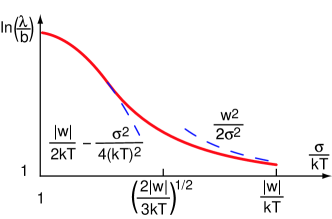
Figure 3: Dependence of antenna length $\lambda$ on the disorder strength $\sigma$. Dashed lines represent the asymptotic limits.

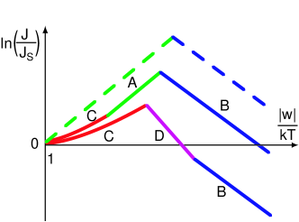
Figure 4: Schematic plot of the dependencies of the rate enhancement $J/J_{s}$ on $|w|$ at $\sigma=\sigma_{1}$ (upper solid curve) and $\sigma=\sigma_{2}$ (lower solid curve). Letters A, B, C, D represent the domains of Fig.2 they go through. Dashed line shows the limit case of the flat energy profile with $\sigma=0$.

The crossover from a relatively weak adsorption to a strong one described by Eqs. (16) again leads to the two scaling regimes for the case of mesoscopic antenna. They are labeled C and D in the diagram Fig. 2. For relatively weak adsorption, when $|w|<\sigma^{2}/kT$, we obtain regime C, where

$$\frac{J}{J_{s}}\sim\exp\left(\frac{w^{2}}{2\sigma^{2}}\right),\ \ \ \ \ ({\rm regime\ C})$$ (21)

while for strong adsorption we have regime D where

$$\frac{J}{J_{s}}\sim\frac{v}{Lb^{2}}\exp\left[-\frac{|w|}{kT}-\frac{\sigma^{2}}{2(kT)^{2}}\right].\ \ \ \ \ ({\rm regime\ D})$$ (22)

In experiment, the adsorption energy $w$ can be controlled by the salt concentration changing the Coulomb part of protein-DNA interaction BWH2 . The dependencies of $\ln(J/J_{s})$ on $|w|$ at the two specified values of disorder strength $\sigma_{1}$ and $\sigma_{2}$ marked in Fig. 2 are schematically plotted in Fig. 4. For comparison, we also plotted the case of the flat energy profile ($\sigma=0$). In both cases with $\sigma>0$, $\ln(J/J_{s})$ first grows proportional to $w^{2}$ (regime C), because the antenna is mesoscopic and thus 1D diffusion is faster, when compared to the normal diffusion at macroscopic antenna. For a relatively small disorder $\sigma=\sigma_{1}$, this rate enhancement continues to regime A but with a rate proportional to $|w|$ because the antenna grows to be macroscopic. For a larger disorder $\sigma=\sigma_{2}$, strong nonspecific adsorption of proteins on distant pieces of DNA slows down the search rate, when the antenna is still mesoscopic, and $\ln(J/J_{s})$ decreases in regime D faster than it does in regime B. The antenna in regime B is macroscopic and $\ln(J/J_{s})$ decreases proportional to $|w|$ for both $\sigma=\sigma_{1}$ and $\sigma=\sigma_{2}$.

The crossover from the weak disorder to the strong one happens at $\sigma\sim\sigma_{0}=kT[(1/2)\ln(v/Lb^{2})]^{1/2}$ (see Fig. 2). If one plugs in the achievable experimental conditions with $L/b\sim 150$ and $v\sim L^{3}$, estimate of $\sigma_{0}$ is the order of $2kT$, which falls in the range of estimates of $\sigma$ from $1kT$ to $6kT$ used in the Refs. Barbi ; Mirny ; Kardar . Apparently $\sigma$ grows for proteins with larger number of contacts with DNA and $\sigma_{0}$ decreases with DNA concentration. In order to identify the role of strong disorder, we look forward to more experiments dealing with relatively large concentrations of short straight DNA to guarantee that disorder strength satisfies $\sigma>\sigma_{0}$.

We know only one observation  BWH2 of the peak in the coordinates of Fig. 4 but for a long and definitely coiled DNA for which our theory is not directly applicable. Indeed, in this paper, we concentrated on the case of relatively short and, therefore, straight DNA. In our recent paper Firstpaper , we presented a general theory including Gaussian coiled and globular DNA in the absence of disorder. In current paper, we did not touch these cases because of our prejudice that simple questions should be addressed first. We concentrated on the simplest regimes labeled A and D in figure 4a of Ref. Firstpaper and still got rather complicated diagram Fig. 2 . That is why we did not try to present our theory for more complicated regimes here.

We are grateful to A.Yu. Grosberg, S.D. Baranovskii and J. Zhang for useful discussions.

References

- (1) M. Ptashne and A. Gann, Genes and signals (Cold Spring Harbor Laboratory Press, Cold Spring Harbor, NY, 2001).
- (2) A.D. Riggs, S. Bourgeois, and M. Cohn. J. Mol. Bol. 53, 401 (1970).
- (3) P.H. Richter and M. Eigen. Biophys. Chem. 2, 255 (1974).
- (4) O.G. Berg, R.B. Winter and P.H. von Hippel. Biochemistry 20, 6929 (1981).
- (5) R.F. Bruinsma. Physica A 313, 211 (2002).
- (6) S.E. Halford and J.F. Marko. Nucleic Acids Res. 32, 3040 (2004).
- (7) S.E. Halford and M.D. Szczelkun. Eur. Biophys. J. 31, 257 (2002).
- (8) K.V. Klenin, H. Merlitz, J. Langowski, C.X. Wu, Phys. Rev. Lett. 96, 018104 (2006).
- (9) Tao Hu, A. Yu. Grosberg and B. I. Shklovskii. Biophys. J. 90, 2731 (2006).
- (10) O.G. Berg and P.H. von Hippel. J. Mol. Biol. 193, 723 (1987).
- (11) U. Gerland, J.D. Moroz and T. Hwa. Proc. Natl. Acad. Sci. USA. 99, 12015 (2002).
- (12) M. Barbi, C. Place, V. Popkov and M. Salerno. Phys. Rev. E 70, 041901 (2004); J. Biol. Phys. 30, 203 (2004).
- (13) K. Nadassy, S.J. Wodak and J. Janin. Biochemistry 38, 1999 (1999).
- (14) M. Slutsky and L.A. Mirny. Biophys. J. 87, 4021 (2004).
- (15) M. Slutsky, M. Kardar and L.A. Mirny. Phys. Rev. E 69, 061903 (2004).
- (16) B.I. Shklovskii and A.L. Efros, Electronic Properties of Doped Semiconductors (Springer-Verlag, Berlin, 1984).
- (17) R.B. Winter, O.G. Berg, and P.H. von Hippel. Biochemistry 20, 6961 (1981).