Andreev drag effect via magnetic quasiparticle focusing in normal-superconductor nanojunctions

Abstract

We study a new hybrid normal-superconductor (NS) $\pi$-junction in which the non-local current can be orders of magnitude larger than that in earlier proposed systems. We calculate the electronic transport of this NS hybrid when an external magnetic field is applied. It is shown that the non-local current exhibits oscillations as a function of the magnetic field, making the effect tunable with the field. The underlying classical dynamics is qualitatively discussed.

Electron-transport properties of normal-superconductor hybrid nanostructures have been the subject of extensive theoretical and experimental experiments attention. Experiments carried out on nanostrucures containing ferromagnets (F) and superconductors (S) reveal novel features, not present in normal-metal/superconductor (N/S) junctions, due to the suppression of electron-hole correlations in the ferromagnet. When spin-flip processes are absent, further effects are predicted, including the suppression of conventional giant magnetoresistance in diffusive magnetic multilayers gmr and the appearance of non-local currents when two fully-polarized ferromagnetic wires with opposite polarizations make contact with a spin-singlet superconductor feinberg . The latter effect, also called the Andreev drag effect, has been highlighted, because of interest in the possibility of generating entangled pairs of electrons at an N-S interface tangle1 . A recent study of such a junction in the tunneling limit feinberg predicts that the magnitude of the non-local current decreases exponentially as $\exp{(-2L/\pi\xi_{c})}$, where $\xi_{c}$ is the superconducting coherence length, and $L$ is the distance between the F contacts. The effect can be enhanced by inserting a diffusive normal conductor between the superconductor and the ferromagnetic contacts leads as shown in Ref. sanchez ; janos . The off-diagonal conductance feinberg , which is always negative in the normal case, can have a positive value of order the contact conductances of these systems. However, the value of the off-diagonal conductance is determined by fixed material parameters, such as the polarization of the ferromagnets, and the spin-flip time in the normal diffusive conductor. Therefore, it is of interest to study alternative methods for material-independent tuning of the non-local current.

In this work, we show that even in the absence of ferromagnetic contacts, an enhanced Andreev drag effect is possible with the N/S structure shown in Fig. 1. We shall demonstrate that the non-local current is enhanced by orders of magnitude compared with the structure in which ferromagnetic leads were used to detect the current feinberg . Moreover, the magnitude of the non-local current can be tuned by varying a magnetic field applied perpendicular to the system. The necessary field is much lower than the critical field of the superconductor.

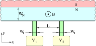
Figure 1: (color online) The hybrid N/S nanostucture consists of an infinitely long N/S ballistic waveguide, comprising a normal (N) metal of width $W_{N}$ coupled to a spin-singlet superconductor (S) region of a width that is much larger than the superconducting coherence length $\xi_{c}$. To measure the non-local current, two ballistic normal leads, at voltages $v_{1}$ and $v_{2}$, and with width $W_{L}$, separated by a distance $L$, are in contact with the normal waveguide. The left and right ends of the waveguide act as drains which absorb any quasi-particles exiting to the left or right. The magnetic field $B$ is applied perpendicular to the system (in our calculation $B>0$ corresponds to a field pointing out of the plane of the system).

To calculate the non-local current we employ the current-voltage relation developed for normal/superconducting hybrid structures in the linear response limit lam1 . Assuming that the voltages $v_{2}$ at lead $2$, is the same as the voltage $v$ of the condensate potential, for the arrangement shown in Fig. 1 one finds that the currents in lead $1$ and $2$ are

$$I_{1} = \frac{2e^{2}}{h}\,\left(N-R_{0}+R_{a}\right)(v_{1}-v),$$ (1a)

$$I_{2} = \frac{2e^{2}}{h}\,\left(T_{a}-T_{0}\right)(v_{1}-v),$$ (1b)

where $v_{1}$ is the voltage at lead $1$ and $N$ is the number of open scattering channels in the normal leads of width $W_{L}$. Here $R_{0}$ ($T_{0}$ ) are the reflection (transmission) coefficients for an electron from lead $1$ to be reflected (transmitted) to lead $1$ ($2$), and $R_{a}$ ($T_{a}$ ) are the Andreev reflection (transmission) coefficients for an electron from lead $1$ to be reflected (transmitted) to lead $1$ ($2$) as a hole. $R_{a}$ and $R_{0}$ satisfy the inequality $N-R_{0}+R_{a}\geq 0$, thus, $I_{1}$ is always positive for positive $v_{1}-v$. All coefficients are evaluated at the Fermi energy using an exact scattering matrix formalism.

It is easy to see from Eq. (1) that whenever Andreev transmission dominates normal transmission (ie $T_{a}>T_{0}$) the currents $I_{1}$ and $I_{2}$ have the same signs, ie a current in lead $1$ induces a current in lead $2$ flowing in the same direction. In semi-classical point of view, this means that hole like quasi-particles leave the system at lead $2$. This is the Andreev drag effect. On the other hand, in the case when the normal transmission is larger than the Andreev transmission (ie $T_{a}<T_{0}$), electron-like quasi-particles leave the system through lead $2$, yielding a current flowing opposite to the direction of the current in lead $1$.

In what follows now, we show that for the system depicted in Fig. 1 the ratio $T_{a}/T_{0}$ can be tuned by an applied magnetic field. To this end, we calculate the transmission coefficients for the system using the Green’s function technique sanvito developed for discrete lattice. Each site is labelled by discrete lattice coordinates $(x,y)$ and possesses particle (hole) degrees of freedom $\psi^{e(h)}(x,y)$. The magnetic field is incorporated via a Peierls substitution. In the presence of local s-wave pairing described by a superconducting order parameter $\Delta(x,y)$, the Bogoliubov-de Gennes equation BdG-eq (BdG) for the retarded Green’s function takes the form

$$\left(\begin{array}[]{cc}\mathbf{H}-E&\Delta\\ \Delta^{\star}&-\mathbf{H}^{\star}+E\end{array}\right)\left(\begin{array}[]{cc}G^{ee}&G^{eh}\\ G^{he}&G^{hh}\end{array}\right)=-\left(\begin{array}[]{cc}\mathbf{1}&\mathbf{0}\\ \mathbf{0}&\mathbf{1}\end{array}\right),$$ (2a)

where the components of $$\bf{H}$$ are

$$\mathbf{H}_{x,x^{\prime},y,y^{\prime}} = \left[\epsilon_{0}-E_{F}\right]\delta_{x,x^{\prime}}\delta_{y,y^{\prime}}-\sum_{n_{x}}\gamma_{x}\delta_{x+n_{x},x^{\prime}}\delta_{y,y^{\prime}}-$$ (2b)

$$- \sum_{n_{y}}\gamma_{y}\delta_{x,x^{\prime}}\delta_{y+n_{y},y^{\prime}}.$$

Here $E_{F}$ is the Fermi-energy, and $n_{x}$ and $n_{y}$ are the nearest neighbors of $(x,y)$ in the $x$ and $y$ direction, respectively.

Within the Landau-gauge with a vector potential in the $x$-direction, $\gamma_{x}=\gamma_{0}e^{i\theta(y)}$, $\gamma_{y}=\gamma_{0}$, where $\gamma_{0}$ is the hopping parameter without magnetic field. The phase $\theta(y)$ for the Peierls substitution is zero in the superconducting region, and it is given by $\theta(y)=Ba^{2}\pi(W_{N}-y)/\Phi_{0}$ in the normal region, where $a$ is the lattice constant parameters:dat , and $\Phi_{0}=h/2e$ is the flux quantum. This choice of gauge results in a uniform magnetic field $B$ in the normal region, and zero magnetic field in the S region, while the translation invariance in the $x$ direction is preserved. The order parameter is assumed to be a step function McMillan ; Plehn , ie constant $\Delta_{0}$ in the S region and zero otherwise. The phase $\theta$ is set to $\theta_{\rm lead}=Ba^{2}\pi W_{N}/\Phi_{0}$ in the leads $1$ and $2$ to ensure the continuity of the vector potential. The parameters of the Hamiltonian $H$ are chosen to model an experimentally-realizable situation in the quasiclassical regime, ie $W_{N}\gg{\rm Fermi\,\,\,wavelength}$ parameters:dat .

From the Green’s function and the scattering matrix for the system, the transmission and reflection coefficients are calculated as a function of the magnetic field. Our central result, shown in Fig. 2, is that the difference between the Andreev and normal transmission coefficients $T_{a}-T_{0}$ (which proportional to the measurable current $I_{2}$ according to Eq. (1b)) is an oscillating function of the magnetic field.

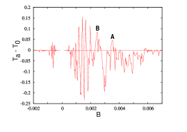
Figure 2: (color online) $T_{a}-T_{0}$ as a function of the magnetic field (in units of $\Phi_{0}/(2a^{2}\pi)$) at the Fermi energy $E_{F}$. In lead $1$ only one mode was allowed. The wave functions at magnetic fields corresponding to letters $A$ and $B$ on the peaks of the curves will be shown in Fig. 5.

Furthermore, since positive peaks correspond to pronounced Andreev drag effect and the heights of the positive peaks are comparable with those of the negative peaks, the non-local current can be as large as the normal current in our hybrid system.

A striking feature of Fig. 2 is that it is an asymmetric function of $B$. This can be understood qualitatively by tracing the classical cyclotron orbits of quasi-particles, bearing in mind that when electron-hole conversion occurs at the NS boundary, the chirality of the electron-like and the hole-like orbits is preserved and therefore a geometrical construction for their classical trajectories is different from that of normal systems zulicke . Examples of trajectories obtained from this new geometrical construction are plotted in Fig. 3.

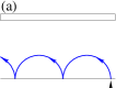
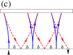
Figure 3: (color online) Classical trajectories in a magnetic field. Figure (a) shows the case when the electron does not reach the N-S interface. New types of trajectories involving Andreev reflections are sketched on figures (b) and (c), for the cases when only the electron (b), both the electron and the hole (c) can reach the side of the waveguide where the leads are attached. Blue (red) lines refer to the electron (hole). Electrons are injected perpendicularly into the waveguide at the positions marked by arrows pointing up.

For $B>0$ electrons injected from lead $1$ will follow classical orbits bending to the left. For a large enough $\left|B\right|$ these will exit to $x=-\infty$, without reaching the N-S interface, and impinging on lead $2$, as can be seen in Fig. 3a. Therefore for large positive $B$ all transmission coefficients from lead $1$ to lead $2$ vanish. Andreev reflection can occur if $|B|$ is sufficiently small to allow the electrons to reach the N-S interface. This condition is defined by $|B|<B_{1}$, where $B_{1}$ is the field for which the cyclotron radius $R_{c}=W_{N}$, where $R_{c}=\sqrt{2mE_{F}}/eB$. As shown in Figs. 3b-c, the transport direction is reversed compared to the normal case due to Andreev scattering, because even if the classical orbits are anti-clockwise, quasi-particle transport is to the right, resulting in quasi-particles impinging on lead 2. This is why the asymmetry in Fig. 2 arises. On the other hand, as shown in Fig. 3b, if $R_{c}$ is not sufficiently large, there is no drag effect, because the trajectories of the holes do not hit the side of the waveguide to which the leads are attached.

Andreev drag effect only occurs for $|B|<B_{\rm max}$, where the maximum field $B_{\rm max}$ is determined from the condition $R_{c}\geq 2W_{N}$. By appropriate choice of the width $W_{N}$ of the normal part of the waveguide, $B_{\rm max}$ can be much less than the critical field of the superconductor. The trajectory relevant for this case is shown in Fig. 3c. On the normal side of the waveguide, normal quasi-particle reflections alternate between electrons and holes, separated by equal distances $\delta$. Assuming that the electrons are injected perpendicularly into the waveguide, simple geometrical considerations give the following condition for maxima in $T_{a}$:

$$L=(2n+1)\delta,$$ (3)

where $n$ is an integer counting the number of normal reflections of the hole at the side of the normal waveguide to which the leads are attached, and $\delta=2\sqrt{R_{c}^{2}-W_{N}^{2}}-\sqrt{R_{c}^{2}-4W_{N}^{2}}-R_{c}$. From Eq. (3) one can find a magnetic field $B_{n}$ for each $n$. The peaks in $T_{a}$ can be expected at $B_{n}$. Taking into account the finite widths of the two leads we calculated the ranges of $B$ for each $n$ in which a peak in $T_{a}$ should be found, which corresponds to the range of $B$ for which a classical trajectory of the hole hits the finite-width interface of lead $2$. In Fig. 4 we plotted the ranges of $B_{n}$ as vertical bars together with those values of magnetic field at which we obtained peaks from the exact quantum calculations.

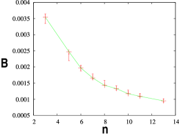
Figure 4: The range of $B_{n}$ shown as a vertical bar for each $n$, together with those values of magnetic field at which we obtained peaks in $T_{a}$ from the quantum transport calculation. (Green line is connecting these peaks, but only for guiding the eyes).

One can see that the agreement between the quantum and the classical calculation is reasonable. Thus, this simple classical argument can be used to estimate the magnetic field needed to obtain enhanced Andreev drag.

To reinforce the above detailed classical picture, we now calculate the electron and hole component of the wave functions inside the N/S waveguide, and compare them with classical orbits. The contribution of the $n$-th incoming mode (from the left N-lead of width $W_{L}$) to the wave function at point ${\bf r}_{S}=(x,y)$ of the waveguide is

$$\psi_{n}^{e(h)}({\bf r}_{S})=\sum_{{\bf r}_{L}}G^{ee(he)}({\bf r}_{S},{\bf r}_{L})\,\chi_{n}^{+,e}({\bf r}_{L}),$$ (4)

where ${\bf r}_{L}$ runs over the surface of the left lead. Here the appropriate components of the retarded Green’s function are defined in Eq. (2a), and $\chi_{n}^{+,e}({\bf r}_{L})$ is the transverse wavefunction of the $n$-th incoming electron channel of the left lead, normalised to unit flux. The modulus square of the electron and hole components of the wave function are shown in Fig. 5 for two different magnetic fields,

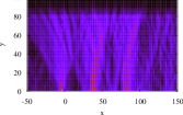
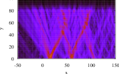
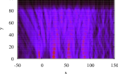
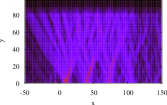
Figure 5: (color online) From top to bottom the electron (left) and hole (right) probability amplitudes are plotted, corresponding to the Andreev-transmission peaks marked by $A$ and $B$ in Fig. 2, respectively. In our geometry $W_{N}=80$, $W=100$, lead $1$ (lead $2$) is located at $-10<x<0$ ($100<x<110$). Distances are in units of the lattice constant parameters:dat .

corresponding to the positive peaks $A$ and $B$ in Fig. 2. For these scattering states, the hole probability amplitude has a local maximum at lead $2$. There are several other maxima of the probability amplitudes of the wave function at the lower side of the waveguide, both for the holes and for the electrons. For each positive peak of ($T_{a}-T_{0}$), the condition Eq. (3) is satisfied, where $n$ is the number of maxima of the hole probability amplitude between the leads, and $\delta$ is the distance between the nearest electron and hole maxima.

In conclusion, we have shown that even in the absence of ferromagnetic leads, an enhanced non-local current can be obtained by including a normal region between the leads and superconductor, and applying magnetic fields perpendicular to the system. The current flowing from lead $1$ to lead $2$ shows oscillations with alternating signs as a function of magnetic field in the small-field regime, corresponding to alternating magnetic focusing of electron and hole-like quasi-particles between the two leads. Unlike an earlier proposal feinberg , where $T_{a}$ is exponentially suppressed with lead separation, the non-local current remains significant even for a lead separation much bigger than the coherence length of the superconductor. We discussed how the quantum results could be interpreted qualitatively in a fully classical treatment providing a better insight into the Andreev drag effect in our system. For the future it would be of interest to extend the semi-classical approach developed for normal focusing problem. In this analysis one has to involve the semi-classical wave functions of the particles taking into account the more complex caustics vanhouten formed for both electrons and holes.

We would like to thank A. F. Morpurgo, C. W. J. Beenakker and A. Kormányos for useful discussions. This work is supported by E. C. Contract No. MRTN-CT-2003-504574, EPSRC, the Hungarian-British TeT, and the Hungarian Science Foundation OTKA TO34832.

References

- (1) S. K. Upadhyay, A. Palanisami, R. N. Louie and R. A. Buhrman, Phys. Rev. Lett. 81, 3247 (1998); S. K. Upadhyay, R. N. Louie and R. A. Buhrman, Appl. Phys. Lett. 74, 3881 (1999); R. J. Soulen et al., Science 282, 85 (1998); C. Fierz, S.-F. Lee, J. Bass, W. P. Pratt Jr and P. A. Schroeder, J. Phys.: Condens. Matter 2, 9701 (1990); M. D. Lawrence and N. Giordano, J. Phys.: Condens. Matter 8, L563 (1996); V. A. Vasko et al., Phys. Rev. Lett. 78, 1134 (1997); M. Giroud, H. Courtois, K. Hasselbach, D. Mailly and B. Pannetier, Phys. Rev. B 58, R11872 (1998); V. T. Petrashov, I. A. Sosnin, I. Cox, A. Parsons and C. Troadec, Phys. Rev. Lett. 83, 3281 (1999); M. D. Lawrence and N. Giordano, J. Phys.: Condens. Matter 11, 1089 (1999); F. J. Jedema et al., Phys. Rev. B 60, 16549 (1999); O. Bourgeois, P. Gandit, J. Lesueur, R. Mélin, A. Sulpice, X. Grison and J. Chaussy, cond-mat/9901045; S. Russo, M. Kroug, T. M. Klapwijk and A. F. Morpurgo, Phys. Rev. Lett. 95, 027002 (2005).
- (2) F. Taddei, S. Sanvito, C.J. Lambert and J.H. Jefferson, Phys. Rev. Lett. 82, 4938 (1999).
- (3) G. Deutscher and D. Feinberg. App. Phys. Lett. 76, 487 (2000); G. Falci, D. Feinberg and F. Hekking, Europhysics Letters 54, 255 (2001).
- (4) G. Bignon, M. Houzet, F. Pistolesi, and F. W. J. Hekking, EuroPhys. Lett. 67, 110 (2004).
- (5) G. B. Lesovik, T. Martin and G. Blatter., Eur. Phys. J. B 24, 287 (2001); N. M. Chtchelkatchev, B. Blatter, G. B. Lesovik and T. Martin, Phys. Rev. B 66, 161320(R) (2002); M. S. Choi, C. Bruder and D. Loss, Phys. Rev. B 62, 13569 (2000); R. Mélin, J. Phys. Condens. Matter 13, 6445 (2001); P. Recher, E. V. Sukhorukov, and D. Loss, Phys. Rev. B 63, 165314 (2001); C. Bena, S. Vishveshwara, L. Balents, and M. P. A. Fisher, Phys. Rev. Lett. 89, 037901 (2002); P. Samuelsson, E. V. Sukhorukov, and M. Büttiker, Phys. Rev. Lett. 91, 157002 (2003) and in New J. Phys. 7, 176 (2005); E. Prada and F. Sols, Eur. Phys. J. B 40, 379-396 (2004) and in New J. Phys. 7, 231 (2005);
- (6) D. Sánchez, R. López, P. Samuelsson and M. Büttiker, Phys. Rev. B 68, 214501 (2003).
- (7) C. J, Lambert, J. Koltai and J. Cserti, in Towards the Controllable Quantum States (Mesoscopic Superconductivity and Spintronics), edited by H. Takayanagi and J. Nitta (World Scientific, Singapore, 2003), pp. 119-125 (cond-mat/0310414).
- (8) C.J. Lambert, J. Phys.: Condens. Matter 3, 6579 (1991); C.J. Lambert, V.C. Hui and S.J. Robinson, J. Phys.: Condens. Matter 5, 4187 (1993); N.K. Allsopp, V.C. Hui, C.J. Lambert and S.J. Robinson, J. Phys.: Condens. Matter 6, 10475 (1994); C.J. Lambert and R. Raimondi, J. Phys. Condensed Matter 10, 901 (1998).
- (9) S. Sanvito, C.J. Lambert, J.H. Jefferson and A.M. Bratkovsky, Phys. Rev. B 59, 11936 (1999).
- (10) P. G. de Gennes, Superconductivity of Metals and Alloys (Benjamin, New York, 1996).
- (11) Throughout the paper we set , , and . For having one open channel in the leads and we set in the leads of width . The Fermi energy is . The separation between leads is . The lattice constant is .
- (12) W. L. McMillan, Phys. Rev. 175, 559 (1968); G. Kieselmann, Phys. Rev. B 35, 6762 (1987).
- (13) H. Plehn, O.-J. Wacker and R. Kümmel, Phys. Rev. B 49, 12140 (1994).
- (14) H. van Houten, C.W.J. Beenakker, J.G. Williamson, M.E.I. Broekaart, P.H.M. van Loodsrecht, B.J. van Wees, J.E. Mooij, C.T. Foxon and J.J. Harris, Phys. Rev. B 39, 8556 (1989).
- (15) F. Giazotto, M. Governale, U. Zülicke, and F. Beltram, Phys. Rev. B 72, 054518 (2005).