Modelling of nematic liquid crystal display devices

Abstract

A lattice Boltzmann scheme is presented which recovers the dynamics of nematic and chiral liquid crystals; the method essentially gives solutions to the Qian-Sheng Qian and Sheng (1998) equations for the evolution of the velocity and tensor order-parameter fields. The resulting algorithm is able to include five independent Leslie viscosities, a Landau-deGennes free energy which introduces three or more elastic constants, a temperature dependent order parameter, surface anchoring and viscosity coefficients, flexo-electric and order electricity and chirality. When combined with a solver for the Maxwell equations associated with the electric field, the algorithm is able to provide a full ‘device solver’ for a liquid crystal display. Coupled lattice Boltzmann schemes are used to capture the evolution of the fast momentum and slow director motions in a computationally efficient way. The method is shown to give results in close agreement with analytical results for a number of validating examples. The use of the method is illustrated through the simulation of the motion of defects in a zenithal bistable liquid crystal device.

I Introduction

Many of the next generation of liquid crystal (LC) display devices use structured or patterned surfaces as an essential element of their design and function Bryan-Brown et al. (2001); Kim et al. (2001); Schift et al. (2002). The correct operation of these devices depends upon the formation and annihilation of defects in the orientational field of the nematic; the defects are usually intimately coupled to a surface. There is also current interest in the behaviour of LC’s with embedded colloidal particles (eg Stark (2001); Loudet et al. (2004)); the behaviour of these materials is frequently dependent upon the interaction of the defects associated with the colloidal particles.

Experimentally it is difficult to obtain information about the spatial and temporal behaviour of the nematic order. Optical methods such as those of Jewell and Sambles (2002, 2003) can, for example, give information about the director profiles on a relatively coarse time and space scale. However, in order to fully understand such systems it is necessary to be able to model the statics and dynamics of a nematic in the presence of complex boundaries and defects. The problem is compounded by the numerous materials parameters needed to fully describe the properties of the LC and its interaction with any bounding surfaces; predictive modelling often requires a fairly complete description of the materials and this therefore necessitates the use of numerical methods to solve the associated equations. In this paper we present the details of one such numerical method and illustrate its use with a number of examples.

LC’s are complex fluids formed from anisometric molecules. These fluids can exhibit a range of mesophases with varying degrees of orientational and positional order of the molecules; in the nematic phase there is long range orientational order but no positional order. The orientational ordering is described at mesoscopic length scales by an order tensor, the Q-tensor (see Section II), whose principal eigenvalue is related to the order parameter and whose principal eigenvector defines the macroscopic director field eg deGennes (1969, 1971); deGennes and Prost (1993). In many systems it is possible to assume that the order parameter is constant and the dynamics of the momentum and director are then described by the well established Ericksen-Leslie-Parodi (ELP) equations (eg deGennes and Prost (1993)).

However, near to bounding walls and close to defects, the assumption of constant order parameter breaks down and the material may also exhibit biaxiality. There are significant spatial gradients in the order tensor in such regions and the gradients have observable macroscopic consequences. For example, Q-tensor gradients lead to the flexo- and order-electric polarisation which is used to control the switching behaviour of some display devices by an applied electric field. Similarly, the dynamics of defects can only be correctly described within a theoretical framework which allows for variation in the order parameter.

In such systems it is necessary to go beyond the ELP theory and adopt a model which describes the dynamics of the full Q-tensor. There are a number of derivations of nematodynamics with variable order parameter (eg Hess (1975); Olmsted and Goldbart (1990); Beris and Edwards (1994); Qian and Sheng (1998)). Work by Sonnet et al Sonnet et al. (2004) provides the basis upon which the variety of schemes with a variable order parameter may be compared; it should be noted that in the limit that the order parameter becomes independent of time and position all the schemes must recover the ELP theory. In this work we adopt the Qian-Sheng Qian and Sheng (1998) formalism because it is straightforward to obtain the required material parameters from those of the equivalent ELP description. Exact solutions to either the ELP or Q-tensor theories are limited to a relatively small number of simplified cases and numerical methods are necessary for the more complex systems which form the focus of this work.

A number of different approaches have been taken to finding numerical solutions to the equations for variable order parameter nemato-dynamics. Svensek Svensek and Zumer (2002) and Fukuda Fukuda et al. (2004) use conventional methods to solve the associated partial differential equations. However, a number of workers have adapted the lattice Boltzmann (LB) method (eg Care and Cleaver (2005); Care et al. (2000); Denniston et al. (2000); Care et al. (2003); Denniston et al. (2004)). Care et al  Care et al. (2000) developed the first methods in which LB was used to solve the ELP equations in a 2-D plane, and later Care et al. (2003) enhanced the method to yield a two dimensional solution to the steady state Qian-Sheng equations; concurrently, Denniston et al   (eg Denniston et al. (2000, 2001, 2004)) developed LB tensor methods for nematic liquid crystals based on the Beris-Edwards Beris and Edwards (1994) scheme.

The LB method may be regarded simply as an alternative method of solving a target set of macroscopic differential equations. However, it is advantageous to regard it as a mesoscale method which allows additional physics to be included within the modelling; this is illustrated by the extension of the method to model the interface between an isotropic and nematic fluid Care et al. (2003), a problem of direct relevance to modelling liquid crystal colloids. LB has the additional stability advantages of being able to incorporate complex boundary conditions more easily than conventional solvers and being straightforward to parallelise.

In this paper we present an LB scheme which recovers the Qian-Sheng equations for nemato-dynamics. The approach modifies the scheme presented in Care et al. (2003) by utilising a simple LBGK scheme (eg Qian et al. (1992)) for the collision term and introducing all the anisotropic behaviour through forcing terms. This moves away from the goal which was implicit in Care et al. (2003) of remaining as close as possible to the physical basis of nematodynamics by using an anisotropic collision operator. However, the overhead in numerical complexity made the scheme difficult to generalise to three dimensions, a restriction which does not apply to the method presented in this paper.

The resulting algorithm includes five independent Leslie viscosities, a Landau-deGennes free energy which introduces three or more elastic constants, a temperature dependent order parameter, surface anchoring and viscosity coefficients, flexo-electric and order electricity and chirality. The precise properties of the system, such as the number of elastic constants, is modified by the inclusion or exclusion of terms in the free energy. When combined with an appropriate solver for the electric field, the algorithm is able to provide a full ‘device solver’ for a liquid crystal display. The method employs two lattice Boltzmann schemes, one for the evolution of the momentum and one for the evolution of the Q-tensor. This is necessary because of the large differences in time scale for the evolution of velocity and director fields in a typical display or experimental arrangement. The paper is organised as follows. In Section II we outline the Qian-Sheng equations for tensor nemato-dynamics. In Section III we present an LB method to recover these equations. In Section IV, results are presented for the validation of the method against analytical equations and the application of the method to the modelling of a Zenithally Bistable Device (ZBD) device is reported. Section V concludes by highlighting the benefits of the method described in the paper and discusses the implications for future work. A Chapman-Enskog analysis (eg Chapman and Cowling (1995)) to justify the LB scheme is given in Appendix A and Appendix B summarises useful relationships between the vector, tensor and LB parameters of the method and lists the material constants used in the simulations detailed in Section IV.

II The Qian-Sheng formalism

In this section we summarise the Qian-Sheng formalism Qian and Sheng (1998) for the flow of a nematic liquid crystal with a variable scalar order parameter. The tensor summation convention is assumed over repeated greek indices which represent three orthogonal Cartesian coordinates; no summation convention is assumed for roman indices which are used to indicate lattice directions of the LB algorithm. $\delta_{\alpha\beta}$ and $\varepsilon_{\alpha\beta\gamma}$ are the Kronecker delta and Levi-Civita symbols respectively and a superposed dot ( ${}^{\dot{}}$ ) denotes the material time derivative: $\partial_{t}+u_{\alpha}\partial_{\alpha}$.

The symmetric, and traceless, macroscopic order tensor, Q, is defined to be

$$Q_{\alpha\beta}=\frac{S}{2}\left(3\hat{n}_{\alpha}\hat{n}_{\beta}-\delta_{\alpha\beta}\right)+\frac{P_{{}_{B}}}{2}\left(\hat{l}_{\alpha}\hat{l}_{\beta}-\hat{m}_{\alpha}\hat{m}_{\beta}\right)$$ (1)

where $S$ and $P_{{}_{B}}$ are the uniaxial and biaxial order parameters with $\hat{\textbf{\em n}},\hat{\textbf{\em l}}$ and $\hat{\textbf{\em m}}$ being orthogonal unit vectors associated with the principle axes of Q. In the uniaxial approximation $P_{{}_{B}}=0$ and in the ELP approximation the scalar order parameter $S\rightarrow S_{0}$, a constant. The director, $\hat{\textbf{\em n}}=(\sin\theta\cos\phi,\sin\theta\sin\phi,\cos\theta)$, is the eigenvector corresponding to the largest eigenvalue of Q.

Following  Qian and Sheng (1998), the momentum and order evolution equations for incompressible ($\partial_{\alpha}u_{\alpha}=0$) nemato-dynamics are written as

$$\rho\dot{u}_{\beta}=\partial_{\alpha}\left(-P\delta_{\alpha\beta}+\sigma_{\alpha\beta}^{v}+\sigma_{\alpha\beta}^{d}+\sigma_{\alpha\beta}^{EM}\right)$$ (2)

$$J\ddot{Q}_{\alpha\beta}=h_{\alpha\beta}+h_{\alpha\beta}^{v}-\lambda\delta_{\alpha\beta}-\varepsilon_{\alpha\beta\gamma}\lambda_{\gamma}$$ (3)

Here the local variables are $\rho$ the liquid crystal density, u the fluid velocity, $P$ the pressure, $J$ the moment of inertia. $\lambda$ and $\lambda_{\gamma}$ are Lagrange multipliers chosen to ensure that Q remains symmetric and traceless. $\sigma_{\alpha\beta}^{d}$ and $h_{\alpha\beta}$ are the distortion stress tensor and molecular field defined by the Landau-deGennes free energy, $F$, for the system through the expressions

$$\sigma_{\alpha\beta}^{d}=-\frac{\partial F_{Bulk}}{\partial(\partial_{\alpha}Q_{\mu\nu})}\partial_{\beta}Q_{\mu\nu}$$ (4)

$$h_{\alpha\beta}=-\frac{\partial F_{Bulk}}{\partial Q_{\alpha\beta}}+\partial_{\gamma}\frac{\partial F_{Bulk}}{\partial(\partial_{\gamma}Q_{\alpha\beta})}$$ (5)

$\sigma_{\alpha\beta}^{v}$ and $h_{\alpha\beta}^{v}$ are the viscous stress tensor and viscous molecular field respectively and are defined by

$$\sigma_{\alpha\beta}^{v} = \beta_{1}Q_{\alpha\beta}Q_{\mu\nu}A_{\mu\nu}+\beta_{4}A_{\alpha\beta}+\beta_{5}Q_{\alpha\mu}A_{\mu\beta}$$ (6)

$$+\beta_{6}Q_{\beta\mu}A_{\mu\alpha}+\frac{\mu_{2}N_{\alpha\beta}}{2}-\mu_{1}Q_{\alpha\mu}N_{\mu\beta}$$

$$~{}~{}~{}~{}~{}~{}~{}+\mu_{1}Q_{\beta\mu}N_{\mu\alpha}$$

$$h_{\alpha\beta}^{v}=-\frac{1}{2}\mu_{2}A_{\alpha\beta}-\mu_{1}N_{\alpha\beta}$$ (7)

Here $\beta_{i},\>\mu_{i}$ are equivalent to the ELP viscosities, $N_{\alpha\beta}$ is the co-rotational derivative, $N_{\alpha\beta}=\dot{Q}_{\alpha\beta}-\varepsilon_{\alpha\mu\nu}\omega_{\mu}Q_{\nu\beta}-\varepsilon_{\beta\mu\nu}\omega_{\mu}Q_{\alpha\nu}$. $A_{\alpha\beta}=\frac{1}{2}\left(\partial_{\alpha}u_{\beta}+\partial_{\beta}u_{\alpha}\right)$ and $W_{\alpha\beta}=\frac{1}{2}\left(\partial_{\alpha}u_{\beta}-\partial_{\beta}u_{\alpha}\right)$ are the symmetric and anti-symmetric velocity gradient tensors with the vorticity being $\omega_{\gamma}=\frac{1}{2}\varepsilon_{\gamma\alpha\beta}W_{\alpha\beta}$. $\sigma_{\alpha\beta}^{EM}$ is the stress tensor arising from externally applied electromagnetic fields Kloos (1999)

$$\sigma_{\alpha\beta}^{EM} = \frac{1}{2}\left(H_{\alpha}B_{\beta}+H_{\beta}B_{\alpha}\right)-\frac{H_{\gamma}B_{\gamma}}{2}\delta_{\alpha\beta}$$ (8)

$$+\frac{1}{2}\left(E_{\alpha}D_{\beta}+E_{\beta}D_{\alpha}\right)-\frac{E_{\gamma}D_{\gamma}}{2}\delta_{\alpha\beta}$$

where $\textbf{\em E}~{}(\textbf{\em H})$ is the electric (magnetic) field strength, D the electric displacement vector and B the magnetic flux density.

Direct calculation of the trace and off-diagonal elements of Eq. (3) shows that lagrange multipliers are given by $\lambda=\frac{1}{3}\left(h_{\gamma\gamma}-\frac{1}{2}\mu_{2}A_{\gamma\gamma}\right)$ and $\lambda_{\gamma}=\frac{1}{2}\varepsilon_{\alpha\beta\gamma}h_{\alpha\beta}$. The term in $A_{\gamma\gamma}$ is included in order to correct the small compressibility errors that arise in LB techniques when the condition upon the Mach number (velocity to speed of sound ratio), $M\equiv|\textbf{\em u}|/c_{s}\ll 1$ is violated.

Order of magnitude estimates and experiments both show the influence of the moment of inertia to be negligible; we therefore set $J=0$ in Eq. (3). Following Care et al. (2000), the viscous stress tensor and the equation of motion Eq. (3) are recast in a form more suitable for the LB development,

$$\sigma_{\alpha\beta}^{v} = \beta_{1}Q_{\alpha\beta}Q_{\mu\nu}A_{\mu\nu}+\beta_{4}A_{\alpha\beta}+\beta_{5}Q_{\alpha\mu}A_{\mu\beta}$$ (9)

$$+\beta_{6}Q_{\beta\mu}A_{\mu\alpha}+\frac{\mu_{2}h_{\alpha\beta}}{2\mu_{1}}-\frac{\mu_{2}\lambda\delta_{\alpha\beta}}{2\mu_{1}}-\frac{\mu_{2}\varepsilon_{\alpha\beta\gamma}\lambda_{\gamma}}{2\mu_{1}}$$

$$-\frac{\mu_{2}^{2}A_{\alpha\beta}}{4\mu_{1}}-Q_{\alpha\mu}h_{\mu\beta}+Q_{\alpha\mu}\varepsilon_{\mu\beta\gamma}\lambda_{\gamma}+\frac{\mu_{2}Q_{\alpha\mu}A_{\mu\beta}}{2}$$

$$+Q_{\beta\mu}h_{\mu\alpha}-Q_{\beta\mu}\varepsilon_{\mu\alpha\gamma}\lambda_{\gamma}-\frac{\mu_{2}Q_{\beta\mu}A_{\mu\alpha}}{2}$$

$$\dot{Q}_{\alpha\beta} = \frac{h_{\alpha\beta}}{\mu_{1}}-\frac{\lambda\delta_{\alpha\beta}}{\mu_{1}}-\frac{\varepsilon_{\alpha\beta\gamma}\lambda_{\gamma}}{\mu_{1}}-\frac{\mu_{2}A_{\alpha\beta}}{2\mu_{1}}$$ (10)

$$+\varepsilon_{\alpha\epsilon\lambda}\omega_{\epsilon}Q_{\lambda\beta}+\varepsilon_{\beta\epsilon\lambda}\omega_{\epsilon}Q_{\alpha\lambda}$$

The derivation of expressions for the molecular field and distortion stress tensor follows the phenomenological approaches for the free energy of liquid crystals Barbero and Evangelista (2001). The global free energy density is considered to be a sum of contributions arising from a number of different physical phenomena $\mathcal{F}_{Global}=\int F_{Bulk}\;d\textbf{\em r}+\int F_{Surface}\;d\textbf{\em S}$. The free energy densities have the form

$$F_{Bulk} = F_{LdG}+F_{Elastic}+F_{Electric}$$ (11)

$$+F_{Magnetic}+F_{Flexo}$$

where

$$F_{LdG} = F_{iso}+\frac{1}{2}\alpha_{F}Q_{\alpha\beta}Q_{\beta\alpha}-\beta_{F}Q_{\alpha\beta}Q_{\beta\gamma}Q_{\gamma\alpha}$$ (12)

$$+\gamma_{F}Q_{\alpha\beta}Q_{\beta\alpha}Q_{\mu\nu}Q_{\nu\mu}$$

$$F_{Elastic} = \frac{1}{2}L_{1}\partial_{\mu}Q_{\nu\gamma}\partial_{\mu}Q_{\nu\gamma}+\frac{1}{2}L_{2}\partial_{\mu}Q_{\nu\mu}\partial_{\gamma}Q_{\nu\gamma}$$ (13)

$$+\frac{1}{2}L_{3}\partial_{\mu}Q_{\nu\gamma}\partial_{\gamma}Q_{\nu\mu}+\frac{1}{2}L_{4}Q_{\mu\nu}\partial_{\mu}Q_{\gamma\tau}\partial_{\nu}Q_{\gamma\tau}$$

$$+\frac{4\pi L_{1}}{P_{ch}}\varepsilon_{\mu\nu\gamma}Q_{\mu\tau}\partial_{\nu}Q_{\gamma\tau}$$

$$-\frac{4\pi L_{4}}{P_{ch}}\varepsilon_{\mu\nu\gamma}Q_{\mu\eta}Q_{\eta\tau}\partial_{\nu}Q_{\gamma\tau}$$

$$+\frac{6\pi^{2}}{P_{ch}^{2}}\left(L_{1}Q_{\mu\nu}Q_{\nu\mu}-L_{4}Q_{\mu\nu}Q_{\nu\tau}Q_{\tau\mu}\right)$$

$$F_{Electric} = -\frac{1}{3}\epsilon_{0}\epsilon_{a}^{max}E_{\alpha}Q_{\alpha\beta}E_{\beta}-\frac{1}{6}\epsilon_{a}\epsilon_{\gamma\gamma}E^{2}$$ (14)

$$F_{Magnetic} = -\frac{1}{3}\mu_{0}\chi_{a}^{max}H_{\alpha}Q_{\alpha\beta}H_{\beta}-\frac{1}{6}\mu_{0}\chi_{\gamma\gamma}H^{2}$$ (15)

$$F_{Flexo} = -\xi_{1}E_{\alpha}\partial_{\gamma}Q_{\alpha\gamma}-\xi_{2}E_{\alpha}Q_{\alpha\gamma}\partial_{\mu}Q_{\gamma\mu}$$ (16)

$$F_{Surface} = \frac{W}{2}\left(Q_{\alpha\beta}-Q_{\alpha\beta}^{o}\right)^{2}$$ (17)

The coefficients $\alpha_{F},\beta_{F},\gamma_{F}$ are parameters controlling the phase of the thermotropic liquid crystal, the negative (positive) sign preceding the $\beta_{F}$ term dictates a calamatic (discotic) state; for biaxial phases sixth order terms are used. $L_{i},~{}i=1\dots 4$, determine the elastic constants. $P_{ch}$ is the pitch of any chirality with $\mu_{0}\left(\epsilon_{0}\right)$ being the permeability(permittivity) of free space. $\chi$  and $\epsilon$ are the diamagnetic and dielectric tensors with $\chi_{a}^{max}\left(\epsilon_{a}^{max}\right)$ the maximal diamagnetic (dielectric) anisotropy (ie $S=1$). $\xi_{1}$ and $\xi_{2}$ are flexoelectric constants, $W$ an anchoring strength and $Q_{\alpha\beta}^{0}$ a preferred surface state. This form for the free energy maintains consistency with the Q-tensor dynamics equations Qian and Sheng (1998) in that a direct analogy with the experimental ELP parameters is made (see Appendix B for the relation between experimental ELP values and the Q-tensor method).

To close the governing equations at surfaces, non-slip boundary conditions are imposed upon the velocity. For infinitely strong anchoring a Q is specified according to Eq. (1). In cases of weak anchoring the order tensor at the surface evolves according to

$$\mu_{S}\partial_{t}Q_{\alpha\beta}=h_{\alpha\beta}^{S}-\lambda^{S}\delta_{\alpha\beta}-\varepsilon_{\alpha\beta\gamma}\lambda_{\gamma}^{S}$$ (18)

where $h_{\alpha\beta}^{S}=-\frac{\partial F_{Bulk}}{\partial\left(\partial_{\tau}Q_{\alpha\beta}\right)}\hat{\nu}_{\tau}-\frac{\partial F_{Surface}}{\partial Q_{\alpha\beta}}$, $\lambda^{S}=\frac{1}{3}h_{\gamma\gamma}^{S}$, $\lambda_{\gamma}^{S}=\frac{1}{3}\varepsilon_{\alpha\beta\gamma}h_{\alpha\beta}^{S}$, $\hat{\nu}$ is an outward pointing surface unit normal vector and $\mu_{S}$ is the surface viscosity defined through $\mu_{S}=\mu_{1}l_{S}$ where $l_{S}$ is a characteristic surface length typically being in the range $l_{S}\approx 100\AA\rightarrow 1000\AA$ Vilfan et al. (2001).

A non-dimensionalisation of the governing equations with respect to characteristic velocity, $\bar{U}$, length , $\bar{L}$, viscosity, $\eta_{eff}=\frac{1}{2}\left(\beta_{4}-\frac{\mu_{1}^{2}}{4\mu_{1}}\right)$, and elastic constant, $\bar{L}_{1}$, yields three key dimensionless numbers which govern the dynamics of the momentum, director, and order parameter respectively

$$\begin{array}[]{lll}Re=\frac{\rho\bar{U}\bar{L}}{\eta_{eff}}&,&\bar{\tau_{p}}=\frac{\rho\bar{L}^{2}}{\eta_{eff}}\\ Er=\frac{\mu_{1}\bar{U}\bar{L}}{\bar{L}_{1}}&,&\bar{\tau_{n}}=\frac{\mu_{1}\bar{L}^{2}}{\bar{L}_{1}}\\ De=\frac{\mu_{1}\bar{U}}{\alpha_{F}\bar{L}}&,&\bar{\tau_{s}}=\frac{\mu_{1}}{\alpha_{F}}\end{array}$$ (19)

The characteristic timescales, $\bar{\tau}$, for variations in the momentum, director and order parameter are also given. $Re$ and $Er$ are the Reynolds and Ericksen numbers. $De$ is the ratio of the relaxation time for the order parameter, $\mu_{1}/\alpha_{F}$, to a time scale associated with the flow, $\bar{L}/\bar{U}$; it is similar to a Deborah number. Considering typical device parameters, $\rho\sim 10^{3}\rm{kg\>m^{-3}}$, $\eta_{eff}\sim 10^{-2}\rm{kg\>m^{1}\>s^{-1}}$, $\bar{L}\sim 10^{-6}\rm{m}$, $\bar{U}\sim 10^{-6}\rm{m\>s^{-1}}$, $\bar{L}_{1}\sim 10^{-12}\rm{kg\>m\>s^{-2}}$ and $\alpha_{F}\sim 10^{5}\rm{kg\>m^{-1}\>s^{-2}}$, we may estimate $\bar{\tau}_{p}\sim 10^{-7}$ s, $\bar{\tau}_{n}\sim 10^{-2}$ s, $\bar{\tau}_{s}\sim 10^{-7}$ s. It is apparent the relaxation rate of the momentum compared to the director is much quicker, as is the relaxation of the order compared to the director and accounting for these timescale differences is essential for dynamic calculations.

III The Algorithm

We proceed now to describe the LB method which recovers the set of equations set out in Sec. II. The algorithm is defined in Sec. III.1. In Sec. III.2 we address the different timescales involved in liquid crystals’ dynamics and how to implement these in the LB method. A Chapman-Enskog multi-scale analysis of the LB algorithm is given in Appendix A.

III.1 Statement Of The Algorithm

LBGK algorithms (eg  Qian et al. (1995)) are well established for solving the Navier Stokes equations for isotropic fluids Dupin et al. (2004). In order to recover the Qian-Sheng equations of Sec II we introduce two LBGK algorithms, one for the evolution of the momentum based on a scalar density $f_{i}\left(\textbf{\em x},t\right)$ and a second LBGK scheme based on a tensor density $g_{i\alpha\beta}\left(\textbf{\em x},t\right)$ to recover the order tensor evolution. It is important distinguish between SI symbols in Sec. II and the symbols used in the LB algorithms, which are defined in terms of lattice units. However in this section, and Sec. Appendix A, this distinction is ignored for clarity. In Sec. III.2 and Appendix B the distinction becomes important and a prime is used to denote a lattice value. Further, a superscript ^P (^Q) is used to distinguish between momentum (order) algorithms.

The principal reason for separating the momentum and order evolution algorithms is the very large difference in time scales between the two processes noted above. In each algorithm, forcing terms are used to recover the required additional terms in the stress tensor and order evolution equations. This approach is more straightforward to implement than the anisotropic scattering method used in an earlier work Care et al. (2003).

The LBGK algorithm for an isotropic fluid may be written in the form

$$f_{i}\left(\textbf{\em x}+\textbf{\em c}_{i}\triangle t,t+\triangle t\right)=f_{i}\left(\textbf{\em x},t\right)$$

$$~{}~{}~{}~{}~{}~{}~{}-\frac{1}{\tau_{{}_{P}}}\left(f_{i}\left(\textbf{\em x},t\right)-f_{i}^{(eq)}\left(\textbf{\em x},t\right)\right)+\phi_{i}\left(\textbf{\em x},t\right)$$

where $f_{i}\left(\textbf{\em x},t\right)$ is the distribution function for particles with velocity $\textbf{\em c}_{i}$ at position x and time $t$, and $\triangle t$ is the time increment. $f_{i}^{(eq)}\left(\textbf{\em x},t\right)$ is the equilibrium distribution function and $\tau_{{}_{P}}$ is the LBGK relaxation parameter. The algorithm fluid density and velocity are determined by the moments of the distribution function,

$$\sum_{i}f_{i}\left[\begin{array}[]{c}1\\ c_{i\alpha}\\ \end{array}\right]\;\;=\;\left[\begin{array}[]{c}\rho(\textbf{\em x},t)\\ \rho u_{\alpha}(\textbf{\em x},t)\\ \end{array}\right]$$ (21)

The mesoscale equilibrium distribution function appropriate to recover the correct hydrodynamics of incompressible fluids ($M\ll 1$) is,

$$f_{i}^{(eq)}=t_{i}\rho\left[1+\frac{c_{i\alpha}u_{\alpha}}{c_{s}^{2}}+u_{\alpha}u_{\beta}\left(\frac{c_{i\alpha}c_{i\beta}-c_{s}^{2}\delta_{\alpha\beta}}{2c_{s}^{4}}\right)\right]$$ (22)

where $t_{i}$ are lattice weights. $t_{i}$, $\textbf{\em c}_{i}$, $c_{s}$ are all dependant upon the choice of lattice, appropriate values of these parameters are summarised in Dupin et al. (2004). An analysis of the standard isotropic algorithm identifies the lattice pressure and kinematic viscosity to be given by

$$P=\rho c_{s}^{2}\;\;\;\;\;\;\;\;\;\;\;\;\;\;\;\;\;\;\;\nu=\frac{c_{s}^{2}}{2}\left(2\tau_{{}_{P}}-1\right)\triangle t$$ (23)

$\phi_{i}$ is a forcing term which is chosen to recover the required terms in the stress tensor. For a nematic liquid crystal governed by Eq. (2) it is defined to be

$$\phi_{i}=t_{i}c_{i\lambda}\partial_{\beta}F_{\beta\lambda}$$ (24)

where

$$F_{\alpha\beta} = \frac{\triangle t}{c_{s}^{2}}\left[\sigma_{\alpha\beta}^{d}+\sigma_{\alpha\beta}^{EM}+\beta_{1}Q_{\alpha\beta}Q_{\mu\nu}A_{\mu\nu}\right.$$ (25)

$$+\beta_{5}Q_{\alpha\mu}A_{\mu\beta}+\beta_{6}Q_{\beta\mu}A_{\mu\alpha}+\frac{\mu_{2}h_{\alpha\beta}}{2\mu_{1}}$$

$$-\frac{\mu_{2}\varepsilon_{\alpha\beta\gamma}\lambda_{\gamma}}{2\mu_{1}}-Q_{\alpha\mu}h_{\mu\beta}+Q_{\alpha\mu}\varepsilon_{\mu\beta\gamma}\lambda_{\gamma}$$

$$+\frac{\mu_{2}Q_{\alpha\mu}A_{\mu\beta}}{2}+Q_{\beta\mu}h_{\mu\alpha}-Q_{\beta\mu}\varepsilon_{\mu\alpha\gamma}\lambda_{\gamma}-$$

$$\left.\frac{\mu_{2}Q_{\beta\mu}A_{\mu\alpha}}{2}\right]$$

with analysis identifying (see Appendix A.1)

$$P=\rho c_{s}^{2}+\frac{\mu_{2}\lambda}{2\mu_{1}}~{};~{}~{}\rho c_{s}^{2}\left(2\tau_{{}_{P}}-1\right)\triangle t=\beta_{4}-\frac{\mu_{2}^{2}}{4\mu_{1}}$$ (26)

and a macroscopic observable velocity of $\rho v_{\alpha}\equiv\sum_{i}f_{i}c_{i\alpha}+(\triangle t/2)\partial_{\beta}F_{\beta\alpha}$. The latter redefinition of the velocity is necessary to reduce higher order artifacts which are introduced by a position dependent forcing term Guo et al. (2002).

To recover the order evolution Eq. (10) we retain the simple LBGK form but replace the scalar density $f_{i}\left(\textbf{\em x},t\right)$ with a symmetric tensor distribution $g_{i\alpha\beta}\left(\textbf{\em x},t\right)$ evolving according to

$$g_{i\alpha\beta}\left(\textbf{\em x}+\textbf{\em c}_{i}\triangle t,t+\triangle t\right)=g_{i\alpha\beta}\left(\textbf{\em x},t\right)$$

$$-\frac{1}{\tau_{{}_{Q}}}\left(g_{i\alpha\beta}\left(\textbf{\em x},t\right)-g_{i\alpha\beta}^{(eq)}\left(\textbf{\em x},t\right)\right)+\chi_{i\alpha\beta}\left(\textbf{\em x},t\right)$$

Here $g_{i\alpha\beta}^{(eq)}\left(\textbf{\em x},t\right)$ is the equilibrium order distribution function and $\tau_{{}_{Q}}$ the LBGK relaxation parameter for the order evolution. The lowest moment of the order distribution function, and its associated equilibrium function, are defined to recover the order tensor of unit trace, $S_{\alpha\beta}$

$$S_{\alpha\beta}=\sum_{i}g_{i\alpha\beta}=\sum_{i}g_{i\alpha\beta}^{(eq)}$$ (28)

which is simply related to the dimensionless zero trace order parameter Q through the relation

$$Q_{\alpha\beta}=\frac{3S_{\alpha\beta}-\delta_{\alpha\beta}}{2}.$$ (29)

The equilibrium order distribution is taken to be

$$g_{i\mu\nu}^{(eq)} = t_{i}S_{\mu\nu}\left[1+\frac{c_{i\alpha}u_{\alpha}}{c_{s}^{2}}\right.$$ (30)

$$\left.~{}~{}~{}~{}+u_{\alpha}u_{\beta}\left(\frac{c_{i\alpha}c_{i\beta}-c_{s}^{2}\delta_{\alpha\beta}}{2c_{s}^{4}}\right)\right]$$

$t_{i},c_{i\alpha},c_{s}^{2}$ are the same lattice parameters defined for the momentum evolution. The forcing term $\chi_{i\alpha\beta}$ is chosen to provide the rotational forces required correctly to recover Eq. (10)

$$\begin{array}[]{rc}\chi_{i\alpha\beta}=\frac{2t_{i}\triangle t}{3}\left[\frac{h_{\alpha\beta}}{\mu_{1}}-\frac{L_{1}\partial_{\lambda}\partial_{\lambda}Q_{\alpha\beta}}{\mu_{1}}-\frac{\lambda\delta_{\alpha\beta}}{\mu_{1}}-\frac{\varepsilon_{\alpha\beta\gamma}\lambda_{\gamma}}{\mu_{1}}\right.\\ \left.-\frac{\mu_{2}A_{\alpha\beta}}{2\mu_{1}}+\varepsilon_{\alpha\epsilon\lambda}\omega_{\epsilon}Q_{\lambda\beta}+\varepsilon_{\beta\epsilon\lambda}\omega_{\epsilon}Q_{\alpha\lambda}\right]\end{array}$$ (31)

The analysis (see Sec. A.2) identifies the key relation

$$\frac{c_{s}^{2}}{2}\left(2\tau_{{}_{Q}}-1\right)\triangle t=\frac{L_{1}}{\mu_{1}}$$ (32)

The scheme described here involves two coupled LB algorithms. Both may be run independently; for example if the effect of flow is to be ignored or only static equilibrium configurations are desired, running the $g_{i\alpha\beta}$ scheme alone will suffice. In practice for typical device geometries, the flow fields evolve on a much faster time scale than the director field; to model such systems the momentum is evolved to steady state between each time step of the order evolution equation. Although the time taken for the momentum to reach equilibrium is significantly shorter than the time step of the order evolution equation, the loss of accuracy in this approach is small.

III.2 Timescales In The Algorithm

Constructing an analogous set of dimensionless numbers to Eq. (19) in terms of the algorithm parameters, from Eqs. (51) and (A.2) results in

$$\begin{array}[]{lll}Re^{\prime}=\frac{2\bar{U}^{\prime_{P}}\bar{L}^{\prime_{P}}}{c_{s}^{2}(2\tau_{{}_{P}}-1)}&,&\bar{\tau_{p}}^{\prime}=\frac{2\bar{L}^{\prime_{P}2}}{c_{s}^{2}(2\tau_{{}_{P}}-1)}\\ Er^{\prime}=\frac{2\bar{U}^{\prime_{Q}}\bar{L}^{\prime_{Q}}}{c_{s}^{2}(2\tau_{{}_{Q}}-1)}&,&\bar{\tau_{n}}^{\prime}=\frac{2\bar{L}^{\prime_{Q}2}}{c_{s}^{2}(2\tau_{{}_{Q}}-1)}\\ De^{\prime}=\frac{\mu_{1}^{\prime_{Q}}\bar{U}^{\prime_{Q}}}{\alpha_{F}^{\prime_{Q}}\bar{L}^{\prime_{Q}}}&,&\bar{\tau_{s}}^{\prime}=\frac{\mu_{1}^{\prime}}{\alpha_{F}^{\prime_{Q}}}\end{array}$$ (33)

We choose $\tau_{{}_{P}}=\tau_{{}_{Q}}=1$ and $\bar{L}^{\prime_{P}}=\bar{L}^{\prime_{Q}}\sim\bar{L}\sqrt{\frac{\left.2\frac{\partial^{2}F_{LdG}}{\partial S^{2}}\right|_{S_{0}}}{3\bar{L}_{1}}}$. The latter identity sets the simulation size to resolve variations in Q. The correct dynamics are achieved by matching the algorithm dimensionless numbers Eq. (33) to the real dimensionless numbers Eq. (19). From Eq. (33) this requires that $\bar{U}^{\prime_{P}}$ differs from $\bar{U}^{\prime_{Q}}$ by an amount $Er/Re$. In order to recover an internally consistent simulation, these different values of the LB velocities in the momentum and order evolution algorithms require the forces to be appropriately scaled when information is passed between the two algorithms. A list of the scaling is given in Appendix B.

We may now take the ratio of characteristic SI to LB times to give the time value of the LB discrete time step. Using typical values shows that: $\triangle t_{{}_{P}}\sim 10^{-13}$ s, $\triangle t_{n}\sim 10^{-8}$ s, $\triangle t_{{}_{S}}\sim 10^{-8}$ s. Hence the momentum algorithm needs to be iterated many times within a single iteration of the order algorithm. Alternatively for laminar creeping flows, $Re\ll 1$, the equilibrium flow field will be reached in a small number of $\triangle t_{{}_{P}}$ and we may jump forward in time to the next $\triangle t_{n}\sim\triangle t_{{}_{S}}$ reducing the overall processing time.

IV Results

In this section we begin by presenting results which validate the algorithm developed above by comparing its numerical predictions with analytical results for some simple cases. We then show how the technique may be used to study the motion of defects in a commonly studied bistable liquid crystal device.

IV.1 Comparison with analytical results for the Miesowicz viscosities

We first consider the flow alignment of the director in a shear flow in the absence of an external aligning field. Provided the channel width is sufficiently large, we may ignore gradients in $Q$ in the centre of the channel. In this case the alignment at the centre of the channel is solely determined by the viscous torque. From Eqs.(1) and (10) we can solve for the director angle, $\theta$, to find

$$\cos(2\theta)=-\frac{\mu_{1}}{\mu_{2}}(3S+P_{{}_{B}})=-\frac{\gamma_{1}}{\gamma_{2}}\left(\frac{S+\frac{1}{3}P_{{}_{B}}}{S_{0}}\right)$$ (34)

A second standard case is to measure the shear viscosity of the nematic in the presence of a strong external field which imposes a fixed director angle. These experiments yield the Miesowicz viscosities deGennes and Prost (1993). However, the standard results must be extended for the case of a variable order parameter. For an arbitrary fixed director angle the effective viscosity, $\eta^{\star}$, is found to be

$$\begin{array}[]{lllllllll}\eta^{\star}&=\frac{\sigma_{\alpha\beta}^{v}}{2A_{\alpha\beta}}\\ &=\frac{\beta_{4}}{2}+\frac{\mu_{2}}{8}S(3n_{1}^{2}-1)-\frac{\mu_{2}}{8}S(3n_{3}^{2}-1)\\ &+\frac{\beta_{5}}{4}S(3n_{3}^{2}-1)+\frac{9\beta_{1}}{4}S^{2}n_{1}^{2}n_{3}^{2}+\frac{\beta_{6}}{4}S(3n_{1}^{2}-1)\\ &+\frac{9\mu_{1}}{2}S^{2}n_{1}^{2}n_{3}^{2}+\frac{9\mu_{1}}{8}S^{2}n_{2}^{2}n_{3}^{2}-\frac{9\mu_{1}}{8}S^{2}n_{1}^{2}n_{2}^{2}\\ &-\frac{\mu_{1}}{4}S^{2}(3n_{1}^{2}-1)(3n_{3}^{2}-1)+\frac{\mu_{1}}{8}S^{2}(3n_{3}^{2}-1)^{2}\\ &+\frac{\mu_{1}}{8}S^{2}(3n_{1}^{2}-1)^{2}\end{array}$$ (35)

from which the following Miesowicz viscosities can be determined:-

$$\left.\begin{array}[]{llll}\eta_{a}=\frac{\beta_{4}}{2}-\frac{\beta_{5}S}{4}-\frac{\beta_{6}S}{4}&\rm{at}\;\hat{n}_{\alpha}=(0,1,0)\\ \eta_{b}=\frac{\beta_{4}}{2}+\frac{3\mu_{2}S}{8}-\frac{\beta_{5}S}{4}+\frac{\beta_{6}S}{2}+\frac{9S^{2}\mu_{1}}{8}&\rm{at}\;\hat{n}_{\alpha}=(1,0,0)\\ \eta_{c}=\frac{\beta_{4}}{2}-\frac{3\mu_{2}S}{8}+\frac{\beta_{5}S}{4}-\frac{\beta_{6}S}{2}+\frac{9S^{2}\mu_{1}}{8}&\rm{at}\;\hat{n}_{\alpha}=(0,0,1)\end{array}\right\}$$ (36)

these being identical to the EL expressions deGennes and Prost (1993) in the limit $S\rightarrow S_{0}$. A biaxial correction is not required as the aligning field serves to cancel biaxial contributions from the shear.

In order to assess the accuracy of the method described in Section III we tested it against these analytical values. We used a channel width $L=1.2\mu\rm{m}$, a shear rate $\dot{\gamma}=10^{4}\rm{s}^{-1}$, viscosities {$\alpha_{1}=-0.011,\>\alpha_{2}=-0.102,\>\alpha_{3}=-0.005,\>\alpha_{4}=0.074,\>\alpha_{5}=0.084,\>\alpha_{6}=-0.023$} $\rm{kg}$ $\rm{m^{-1}}$ $\rm{s^{-1}}$, Landau parameters { $a=65000\>\rm{J\>m^{-3}\>K^{-1}}$, $B=530000\>\rm{J\>m^{-3}}$, $C=980000\>\rm{J\>m^{-3}}$} and $T=T_{IN}-4(T_{IN}-T^{\star})$. The boundaries were assumed to have infinite anchoring and the flow induced by adding $2t_{i}\rho^{w}\underline{c}_{i}\cdot\underline{u}^{w}/(c_{s}^{2})$ to the right hand side of Eq. (III.1) where the wall velocity is $+(-)\underline{u}^{w}$ at the top (bottom) boundaries with periodicity in the $x$ and $y$ directions.

In the absence of an aligning field, the director angle in the shear flow was found to be $12.166^{\circ}$ which agreed with the value predicted by Eq. (34) to 7 significant figures. Accuracy was found to be maintained over all flow aligning viscosity ratio’s with a typical increase in $S$ around $0.002$ and biaxiality $P_{{}_{B}}=0.002$. The Miesowicz viscosities were measured using an aligning field of $75$ volts ($\triangle\epsilon_{a}=10.3$) in the relevant directions. Non-slip boundary conditions were applied using the bounce-back method Dupin et al. (2004)) and the flow was induced by applying a constant body force at $z=L/2$. The resultant viscosity ratio’s are compared in Table 1 where data is measured at $z=L/4$. It can be seen that the LB solver gives results in good agreement with the expected values.

Theory	Simulation	% error
$\eta_{a}/\eta_{b}=1.446$	$\dot{\gamma}_{a}^{-1}/\dot{\gamma}_{b}^{-1}=1.446$	$1.6\times 10^{-4}$
$\eta_{a}/\eta_{c}=0.227$	$\dot{\gamma}_{a}^{-1}/\dot{\gamma}_{c}^{-1}=0.227$	$1.4\times 10^{-4}$
$\eta_{b}/\eta_{c}=0.157$	$\dot{\gamma}_{b}^{-1}/\dot{\gamma}_{c}^{-1}=0.157$	$2.8\times 10^{-5}$

Table 1: Table of theoretical (Eq. (36)) and simulated ratio’s of the Miesowicz viscosities.

IV.2 Investigation of defect motion in a bistable device

The ZBD device Bryan-Brown et al. (2001); Jones et al. (2000) uses a structured surface, such as that in Fig. (1), to introduce bistability which may be used to design a very low power display. The two bistable states are characterised by the presence or absence of defects which will be referred to as the defect ($\mathcal{D}$) and continuous ($\mathcal{C}$) states respectively. One possible method to latch switch between states is to use an electric field that couples to the flexoelectric properties of the liquid crystal material. Latching between the two states is a dynamic process which involves the nucleation and annihilation of defects.

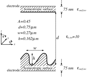
Figure 1: Schematic of the two dimensional ZBD geometry over two grating pitches, $w$. Homeotropic boundary conditions serve to cause bistability. Simulations contain one grating pitch and periodic boundaries in the $x$ and $y$ directions.

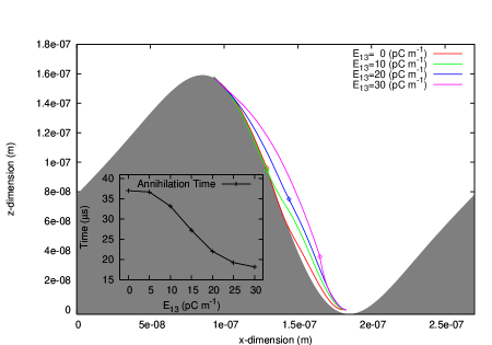
Figure 2: Defect trajectories during the $\mathcal{D}$ to $\mathcal{C}$ latching for various $E_{13}$ values. Points indicate location of the annihilation. The inset figure indicates the time at which defects annihilate from the turn on of the voltage. $\epsilon_{\gamma\gamma}=18$, $V=+18$ volts and $\triangle\epsilon_{a}=10.3$.

We followed  Bryan-Brown et al. (2001) and modelled the ZBD surface with the function $g(x)=h\sin\left[\frac{2\pi x}{w}+A\sin\left(\frac{2\pi x}{w}\right)\right]$ projected onto the LB boundary over one grating period, $w$; the height of the grating is $h$ and the parameter $A$ controls the level of asymmetry. Weak anchoring conditions was used at the surfaces by implementing Eq. (18) with an explicit forward time finite difference method. The gradients in the equation were extrapolated to second order from the bulk and an average taken over the values obtained from each lattice direction. It should be noted that in order to achieve equality of the elastic constants in the bulk and at the surface it is necessary for the surface parameters $L_{i}^{S}$ to be different from bulk LB through the $L_{i}^{S}=L_{i}/(2\tau_{{}_{Q}}-1)$. This arises because the relaxation processes in the bulk, which are governed by the parameter $\tau_{{}_{Q}}$, contribute to the measured elastic constants in the bulk. However, there is no equivalent collision process in the surface algorithm.

In the presence of the voltage applied to the device, it is necessary to solve Maxwell’s equations over the LB grid to obtain the local values for the electric field, E. For completeness these equations are

$$\left.\begin{array}[]{llllllllll}\partial_{\alpha}D_{\alpha}=0\\ D_{\alpha}=\epsilon_{0}\epsilon_{\alpha\beta}E_{\beta}+P_{\alpha}\\ E_{\beta}=-\partial_{\beta}V\\ \epsilon_{\alpha\beta}=(2\triangle\epsilon_{a}^{max}Q_{\alpha\beta}+\epsilon_{\gamma\gamma}\delta_{\alpha\beta})/3\\ \end{array}\right\}$$ (37)

in which $V$ is the local voltage, $\epsilon_{\gamma\gamma}=2\epsilon_{\perp}+\epsilon_{\parallel}$, $\triangle\epsilon_{a}=S\triangle\epsilon_{a}^{max}$ and $P_{\sigma}$ is defined from Eq. (16) by writing it in the form $F_{Flexo}=-P_{\sigma}E_{\sigma}$. We solve equations (37) using a successive overrelaxation method at each iteration of the LB algorithm for $g_{i\alpha\beta}$. This therefore determines the electric field which is consistent with the instantaneous value of the $Q$ tensor.

We investigated the effect of material properties on the motion of defects in this device; in particular we studied the interplay of dielectric, flexoelectric and surface polarisation effects. We used the set of material parameters given in Appendix B. The system was first established at steady state in one of the equilibrium states; the simulation was then run using the algorithm described above. The equilibrium states were located by starting from an appropriate initial condition and running only the $g_{i\alpha\beta}$ algorithm. The defect equilibrium state ($\mathcal{D}$) has a -1/2 defect near the peak of the grating and a +1/2 defect near the trough of the grating.

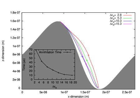
Figure 3: Defect trajectories during the $\mathcal{D}$ to $\mathcal{C}$ latching for various $\triangle\epsilon_{a}$ values. Points indicate location of the annihilation. The inset figure indicates the time at which defects annihilate from the turn on of the voltage. $\epsilon_{\gamma\gamma}=18$, $V=+18$ volts and $E_{13}=20\rm{pC\;m^{-1}}$.

In Fig. (2) the flexoelectric coefficient $E_{13}=\frac{e_{11}+e_{33}}{2}$, ($e_{11}=e_{33}$) is varied. Starting in the $\mathcal{D}$ state and applying $+18$($\mathrm{𝟎}$) volts to the upper (lower) electrodes the resultant defect trajectories are shown in the grating region. For $E_{13}=0$ the defects move slowly along the surface and annihilate. As $E_{13}$ increases we increase the surface polarisation and order parameter which pushes the defects further out into the bulk of the device to annihilate. As $E_{13}$ increases the $-\frac{1}{2}$ defect mobility is increased as seen in the annihilation locations. The inset of Fig. (2) shows the time taken for the defects to annihilate which is an indicator of the latching speed. It is found increasing $E_{13}$ increases the latching speed.

Alternatively we may keep $E_{13}$ constant and vary the dielectric anisotropy, see Fig. (3). For a deceasing $\triangle\epsilon_{a}$ we effectively increase flexoelectric contributions to the nematic (see Eqs. (14)and (16)), this increases the surface polarisation that pushes the defects further away from the surface. Increasing $\triangle\epsilon_{a}$ effectively reduces the flexoelectric contributions and the defects annihilate closer to the surface; this also reduces the latching time.

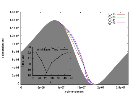
Figure 4: Defect trajectories during the $\mathcal{D}$ to $\mathcal{C}$ latching for various $\epsilon_{\gamma\gamma}^{S}$ values. Points indicate location of the annihilation. The inset figure indicates the time at which defects annihilate from the turn on of the voltage. $\triangle\epsilon_{a}=10.3$, $V=+18$ volts and $E_{13}=20\rm{pC\;m^{-1}}$.

Fig. (4) has fixed $\triangle\epsilon_{a}$ and $E_{13}$ but the grating permittivity $\epsilon_{\gamma\gamma}^{S}$ is changed. This has the effect of diffracting the electric field lines for an increased mis-match of surface and nematic permittivities. At the lower dielectric mismatch the defect annihilation location is at $\sim h/2$. Increasing the dielectric mismatch increases the mobility of the $-\frac{1}{2}$ defect allowing it to travel further and annihilate near the grating trough. There appears to be an optimum value of $\epsilon_{\gamma\gamma}^{S}\sim 26$ for which the annihilation time is shortest.

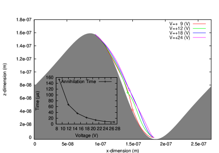
Figure 5: Defect trajectories during the $\mathcal{D}$ to $\mathcal{C}$ latching for various $E_{13}$ values. Points indicate location of the annihilation. The inset figure indicates the time at which defects annihilate from the turn on of the voltage. $\triangle\epsilon_{a}=10.3$, $\epsilon_{\gamma\gamma}=18$ and $E_{13}=20\rm{pC\;m^{-1}}$.

Fig. (5) shows the effect of increasing the applied voltage for constant $\epsilon_{\gamma\gamma}^{S}$, $\triangle\epsilon_{a}$ and $E_{13}$ ; this has the effect of increasing the contributions of both the flexoelectric and dielectric terms. An increased voltage tends to cause the defect trajectories to move away from the surface towards a saturation distance for which further increase causes little difference. Above the voltages shown in the figure, a different latching mode is seen in which several pairs of defects occur in the annihilation process. As with a Fredericksz response an increased voltage results in a faster latching response.

V Conclusions

An LB method has been presented which can be used to predict the dynamics of a nematic liquid crystal in the complex geometries which are increasingly being adopted for display devices. Nematic order, director, velocity, electric fields and surface polarisations are all recovered; this allows comparison to experimental results to be made for a wide range of cell geometries or surface patterning. In the presence of structured surfaces and defects, it is essential to consider the variation in the order parameter. Essentially, a full ‘device solver’ has been developed and example results are given that show both the accuracy of the solver and its use in determining behaviour of next generation LC devices. The influence of surface polarisations resulting from dielectric and flexoelectric effects are shown to effect defect trajectories and ultimately latching speeds. The solver is currently being used in the development of next generation bistable devices.

Appendix A Chapman-Enskog analysis of the LB algorithm

In this section we present a Chapman-Enskog analysis of the momentum and order evolution schemes. This analysis serves two purposes: to demonstrate that the method recovers the required governing equations and to identify the relation of the LBGK parameters to the associated transport coefficients and forcing terms.

A.1 Momentum Evolution

The moments of the distribution function, $f_{i}$, are defined to be

$$\left.\begin{array}[]{lllllllll}\sum_{i}f_{i}^{(0)}\left[\begin{array}[]{ccccc}1\\ c_{i\alpha}\\ c_{i\alpha}c_{i\beta}\end{array}\right]&=&\left[\begin{array}[]{ccccc}\rho\\ \rho u_{\alpha}\\ \Pi_{\alpha\beta}^{(0)}=\rho c_{s}^{2}\delta_{\alpha\beta}+\rho u_{\alpha}u_{\beta}\end{array}\right]\\ \sum_{i}f_{i}^{(n)}\left[\begin{array}[]{ccccc}1\\ c_{i\alpha}\\ c_{i\alpha}c_{i\beta}\end{array}\right]&=&\left[\begin{array}[]{ccccc}0\\ 0\\ \Pi_{\alpha\beta}^{(n)}\end{array}\right]\;\;,\;\;\;\;n>0\end{array}\right\}$$ (38)

The the velocity basis and the $t_{i}$ are chosen to give

$$\left.\begin{array}[]{lll}\sum_{i}t_{i}&=&1\\ \sum_{i}t_{i}c_{i\alpha}&=&0\\ \sum_{i}t_{i}c_{i\alpha}c_{i\beta}&=&c_{s}^{2}\delta_{\alpha\beta}\\ \sum_{i}t_{i}c_{i\alpha}c_{i\beta}c_{i\gamma}&=&0\\ \sum_{i}t_{i}c_{i\alpha}c_{i\beta}c_{i\gamma}c_{i\theta}&=&c_{s}^{4}\Delta_{\alpha\beta\gamma\theta}\end{array}\right\}$$ (39)

where

$$\Delta_{\alpha\beta\gamma\theta}=\delta_{\alpha\beta}\delta_{\gamma\theta}+\delta_{\alpha\gamma}\delta_{\beta\theta}+\delta_{\alpha\theta}\delta_{\beta\gamma}$$ (40)

Using a Taylor expansion on the left hand side of Eq. (III.1) we obtain:

$$\begin{array}[]{ccc}\triangle t\partial_{t}f_{i}+\frac{\triangle t^{2}}{2}\partial_{t}\partial_{t}f_{i}+\triangle tc_{i{\alpha}}\partial_{\alpha}f_{i}+\triangle t^{2}c_{i\alpha}\partial_{t}\partial_{\alpha}f_{i}\\ +\frac{\triangle t^{2}}{2}c_{i\alpha}c_{i\beta}\partial_{\alpha}\partial_{\beta}f_{i}=-\frac{1}{\tau_{{}_{P}}}\left(f_{i}-f_{i}^{(eq)}\right)+\phi_{i}\end{array}$$ (41)

We assume a forcing term $\phi_{i}$ of the form $\phi_{i}=t_{i}c_{i\lambda}\partial_{\beta}F_{\beta\lambda}$ and use a multi-scale expansion, to second order

$$\left.\begin{array}[]{ccc}t_{1}=\varepsilon t\;\;,\;\;\;\;\;t_{2}=\varepsilon^{2}t\;\;,\;\;\;\;\;\partial_{t}=\varepsilon\partial_{t_{1}}+\varepsilon^{2}\partial_{t_{2}}\\ x_{1}=\varepsilon x\;\;,\;\;\;\;\;x_{2}=\varepsilon^{2}x\;\;,\;\;\;\;\;\partial_{x}=\varepsilon\partial_{x_{1}}+\varepsilon^{2}\partial_{x_{2}}\\ f_{i}=f_{i}^{(0)}+\varepsilon f_{i}^{(1)}+\varepsilon^{2}f_{i}^{(2)}\end{array}\right\}$$ (42)

Using this expansion in Eq. (41) and collecting terms we obtain:
$O(\varepsilon^{0})$

$$f_{i}^{(0)}=f_{i}^{(eq)}$$ (43)

$O(\varepsilon^{1})$

$$-\tau_{{}_{P}}\triangle t(\partial_{t_{1}}+c_{i\alpha_{1}}\partial_{\alpha_{1}})f_{i}^{(0)}$$

$$+\tau_{{}_{P}}t_{i}c_{i\lambda}\partial_{\beta_{1}}F_{\beta\lambda} = f_{i}^{(1)}$$ (44)

$O(\varepsilon^{2})$

$$\left(\frac{1}{2}-\tau_{{}_{P}}\right)\triangle t\left(\partial_{t_{1}}+c_{i\alpha}\partial_{\alpha_{1}}\right)f_{i}^{(1)}$$

$$-\tau_{{}_{P}}\triangle t\left(\partial_{t_{2}}+c_{i\alpha}\partial_{\alpha_{2}}\right)f_{i}^{(0)}$$

$$-\frac{\tau_{{}_{P}}\triangle t}{2}\left(\partial_{t_{1}}+c_{i\alpha}\partial_{\alpha_{1}}\right)t_{i}c_{i\lambda}\partial_{\beta_{1}}F_{\beta\lambda}$$

$$+\tau_{{}_{P}}t_{i}c_{i\lambda}\partial_{\beta_{2}}F_{\beta\lambda} = f_{i}^{(2)}$$ (45)

in which we have used the $O(\varepsilon^{1})$ result of Eq. (44) to replace a term of the form $(\partial_{t_{1}}+c_{i\alpha}\partial_{\alpha_{1}})f_{i}^{(0)}$ in the $O(\varepsilon^{2})$ result. Taking the zeroth moment of Eq. (44) and Eq. (45) whilst respecting Eq. (38) yields:

$$\begin{array}[]{lllll}O(\varepsilon^{1})&&&\partial_{t_{1}}\rho+\partial_{\alpha_{1}}\left(\rho u_{\alpha}\right)=0\\ O(\varepsilon^{2})&&&\partial_{t_{2}}\rho+\partial_{\alpha_{2}}\left(\rho u_{\alpha}\right)=c_{s}^{2}\partial_{\gamma_{1}}\partial_{\beta_{1}}F_{\beta\gamma}/2\end{array}$$ (46)

which can be recombined to give the continuity equation:

$$\partial_{t}\rho+\partial_{\alpha}\left(\rho u_{\alpha}\right)=0$$ (47)

where the term $c_{s}^{2}\partial_{\lambda}\partial_{\beta}F_{\beta\lambda}/2$ is corrected for by redefining the macroscopic velocity as described below Eq. (26).

Taking the first moment ($\sum_{i}c_{i\beta}$) of the first and second order Eq. (44) and Eq. (45) whilst respecting Eq. (38) yields:

$$\begin{array}[]{lllll}O(\varepsilon^{1})&&&\partial_{t_{1}}(\rho u_{\beta})+\partial_{\alpha_{1}}\Pi_{\alpha\beta}^{(0)}=\frac{c_{s}^{2}}{\triangle t}\partial_{\gamma_{1}}F_{\gamma\beta}\\ O(\varepsilon^{2})&&&\left(1-\frac{1}{2\tau_{{}_{P}}}\right)\partial_{\alpha_{1}}\Pi_{\alpha\beta}^{(1)}+\partial_{t_{2}}(\rho u_{\beta})\\ &&&+\partial_{\alpha_{2}}\Pi_{\alpha\beta}^{(0)}=\frac{c_{s}^{2}}{\triangle t}\partial_{\gamma_{2}}F_{\gamma\beta}-\frac{c_{s}^{2}}{2}\partial_{t_{1}}\partial_{\gamma_{1}}F_{\gamma\beta}\end{array}$$ (48)

In order to progress, the $\Pi_{\alpha\beta}^{(1)}$ term needs evaluating and this requires knowledge of $f_{i}^{(1)}$ (in Eq. (44)). Using Eq. (22) to $O(\underline{\textbf{\em u}})$ in Eq. (44), taking its zeroth moment and back substituting the result ($\partial_{t_{1}}\rho=-\partial_{\beta_{1}}(\rho u_{\beta})$), followed by taking the first moment and another back substitution ($\partial_{t_{1}}(\rho u_{\beta})=-c_{s}^{2}\partial_{\beta_{1}}\rho-\tau_{{}_{P}}c_{s}^{2}\partial_{\gamma_{1}}F_{\gamma\beta}$) yields

$$f_{i}^{(1)} = -\frac{\tau_{{}_{P}}\triangle t\partial_{\beta_{1}}(\rho u_{\alpha})H_{i\alpha\beta}}{c_{s}^{2}}$$ (49)

$$~{}~{}~{}~{}+\tau_{{}_{P}}t_{i}c_{i\lambda}(\tau_{{}_{P}}\triangle t+1)\partial_{\gamma_{1}}F_{\gamma\lambda}$$

in which the symmetric quantity $H_{i\alpha\beta}$ is given by

$$H_{i\alpha\beta}=t_{i}c_{s}^{2}\left(\frac{c_{i\alpha}c_{i\beta}}{c_{s}^{2}}-\delta_{\alpha\beta}\right)$$ (50)

The symmetry of Eq. (50) allowing us to replace $\partial_{\lambda}(\rho u_{\beta})$ by $\rho A_{\lambda\beta}$ in Eq. (49), in the incompressible limit.

We now use Eq. (49) to evaluate Eqs. (48) and combine the results to find

$$\partial_{t}(\rho u_{\beta})+u_{\alpha}\partial_{\alpha}(\rho u_{\beta})=-\partial_{\beta}(\rho c_{s}^{2})$$ (51)

$$+c_{s}^{2}(2\tau_{{}_{P}}-1)\triangle t\partial_{\alpha}(\rho A_{\beta\alpha})+\frac{c_{s}^{2}}{\triangle t}\partial_{\alpha}F_{\alpha\beta}$$

Here the term $-\frac{c_{s}^{2}}{2}\partial_{t}\partial_{\gamma}F_{\beta\gamma}$ can be neglected assuming high order gradients are negligibly small.

A detailed comparison of the terms in this equation to the target momentum equation Eq. (2) gives the identifications made in Eqs. (26). Note that the isotropic terms may be incorporated into the scalar pressure deGennes and Prost (1993). Comparison of the remaining stress tensor terms allows the forcing term Eq. (25) to be defined. This completes the momentum analysis.

A.2 Order Tensor Evolution

The moments of the order distribution function are defined to be

$$\left.\begin{array}[]{lllccc}\sum_{i}g_{i\alpha\beta}^{(0)}\left[\begin{array}[]{ccccc}1\\ c_{i\gamma}\end{array}\right]&=&\left[\begin{array}[]{ccccc}S_{\alpha\beta}\\ u_{\gamma}S_{\alpha\beta}\end{array}\right]\\ \sum_{i}g_{i\alpha\beta}^{(n)}\left[\begin{array}[]{ccccc}1\\ c_{i\gamma}\end{array}\right]&=&\left[\begin{array}[]{ccccc}0\\ \Omega^{(n)}_{\alpha\beta\gamma}\end{array}\right]\;\;,\;\;\;\;n>0\end{array}\right\}$$ (52)

It should be noted that we adopt a unit trace order tensor in these moment definitions in order to be consistent with  Care et al. (2003). However, since the momentum and order are now in separate algorithms, we could equally well have defined zero trace moment definitions as in Denniston et al. (2000).

Using a Taylor expansion on the left hand side of lattice evolution equation (Eq.(III.1)) we obtain:

$$\begin{array}[]{ccc}\triangle t\partial_{t}g_{i\mu\nu}+\frac{\triangle t^{2}}{2}\partial_{t}\partial_{t}g_{i\mu\nu}+\triangle tc_{i{\alpha}}\partial_{\alpha}g_{i\mu\nu}\\ ~{}~{}~{}+\triangle t^{2}c_{i\alpha}\partial_{t}\partial_{\alpha}g_{i\mu\nu}+\frac{\triangle t^{2}}{2}c_{i\alpha}c_{i\beta}\partial_{\alpha}\partial_{\beta}g_{i\mu\nu}\\ =-\frac{1}{\tau_{{}_{Q}}}\left(g_{i\mu\nu}-g_{i\mu\nu}^{(eq)}\right)+\chi_{i\mu\nu}\end{array}$$ (53)

We suppose the as yet unknown forcing term $\chi_{i\mu\nu}$ will be dependent on the gradient in both u and Q and can be expanded as $\chi_{i\mu\nu}=\varepsilon\chi_{i\mu\nu}^{(1)}+\varepsilon^{2}\chi_{i\mu\nu}^{(2)}$. We augment Eqs. (42) with the expansion

$$\begin{array}[]{ccc}g_{i}=g_{i\mu\nu}^{(0)}+\varepsilon g_{i\mu\nu}^{(1)}+\varepsilon^{2}g_{i\mu\nu}^{(2)}\end{array}$$ (54)

Substituting into the Taylor expansion Eq. (53), we find $O(\varepsilon^{0})$

$$g_{i\mu\nu}^{(0)}=g_{i\mu\nu}^{(eq)}$$ (55)

$O(\varepsilon^{1})$

$$-\tau_{{}_{Q}}\triangle t(\partial_{t_{1}}+c_{i\alpha_{1}}\partial_{\alpha_{1}})g_{i\mu\nu}^{(0)}+\tau_{{}_{Q}}\chi_{i\mu\nu}^{(1)}=g_{i\mu\nu}^{(1)}$$ (56)

$O(\varepsilon^{2})$

$$\left(\frac{1}{2}-\tau_{{}_{Q}}\right)\triangle t\left(\partial_{t_{1}}+c_{i\alpha}\partial_{\alpha_{1}}\right)g_{i\mu\nu}^{(1)}$$

$$-\tau_{{}_{Q}}\triangle t\left(\partial_{t_{2}}+c_{i\alpha}\partial_{\alpha_{2}}\right)g_{i\mu\nu}^{(0)}$$

$$-\frac{\tau_{{}_{Q}}\triangle t}{2}\chi_{i\mu\nu}^{(1)}+\tau_{{}_{Q}}\chi_{i\mu\nu}^{(2)} = g_{i\mu\nu}^{(2)}$$ (57)

in which we have used the $O(\varepsilon^{1})$ result of Eq. (56) to replace a term of the form $(\partial_{t_{1}}+c_{i\alpha}\partial_{\alpha_{1}})g_{i\mu\nu}^{(0)}$ in the $O(\varepsilon^{2})$ result.

Taking the zeroth moment of the first order Eq. (56) expansion and using Eq. (52) gives

$$\partial_{t_{1}}\left(S_{\mu\nu}\right)+\partial_{\alpha_{1}}\left(u_{\alpha}S_{\mu\nu}\right)=\sum_{i}\frac{\chi_{i\mu\nu}^{(1)}}{\triangle t}$$ (58)

which may be written in terms of Q as

$$\partial_{t_{1}}\left(Q_{\mu\nu}\right)+\partial_{\alpha_{1}}\left(u_{\alpha}Q_{\mu\nu}\right)=\frac{3}{2\triangle t}\sum_{i}\chi_{i\mu\nu}^{(1)}$$ (59)

Similarly, the zeroth moment of the second order expansion gives

$$\left(1-\frac{1}{2\tau_{{}_{Q}}}\right)\partial_{\alpha_{1}}\Omega_{\alpha\mu\nu}^{(1)}+\frac{2}{3}\partial_{t_{2}}Q_{\mu\nu}+\frac{2}{3}\partial_{\alpha_{2}}\left(u_{\alpha}Q_{\mu\nu}\right) =$$

$$+\frac{1}{\triangle t}\sum_{i}\chi_{i\mu\nu}^{(2)}-\frac{1}{2}\sum_{i}\chi_{i\mu\nu}^{(1)}~{}~{}~{}~{}~{}$$ (60)

We now need to evaluate $\Omega_{\alpha\mu\nu}^{(1)}$ by obtaining an expression for $g_{i\mu\nu}^{(1)}$ in Eq. (56). We use Eq. (30) to $O(\underline{\textbf{\em u}})$ in Eq.(56). Taking the first moment of this gives

$$\Omega_{\gamma\mu\nu}^{(1)}=\tau_{{}_{Q}}\sum_{i}c_{i\gamma}\chi_{i\mu\nu}^{(1)}-\tau_{{}_{Q}}\triangle t\left[S_{\mu\nu}\partial_{t_{1}}(u_{\gamma})\right.$$

$$\left.+u_{\gamma}\partial_{t_{1}}(S_{\mu\nu})+\partial_{\gamma_{1}}(S_{\mu\nu}c_{s}^{2})\right]$$ (61)

Using the result Eq. (58), we may replace $\partial_{t_{1}}(S_{\mu\nu})$ and find

$$\Omega_{\gamma\mu\nu}^{(1)}=-\tau_{{}_{Q}}\triangle t\biggl{[}S_{\mu\nu}\partial_{t_{1}}(u_{\gamma})-u_{\gamma}\partial_{\alpha_{1}}(u_{\alpha}S_{\mu\nu})\biggr{.}$$

$$\left.+\frac{u_{\gamma}}{\triangle t}\sum_{i}\chi_{i\mu\nu}^{(1)}+\partial_{\gamma_{1}}(S_{\mu\nu}c_{s}^{2})\right]$$

$$+\tau_{{}_{Q}}\sum_{i}c_{i\gamma}\chi_{i\mu\nu}^{(1)}~{}~{}~{}$$ (62)

We may use the result obtained in text above Eq. (49) to find:

$$\partial_{t_{1}}u_{\beta}=-\frac{c_{s}^{2}\partial_{\beta_{1}}\rho-\tau_{{}_{P}}\partial_{\gamma_{1}}F_{\beta\gamma}c_{s}^{2}+u_{\beta}\partial_{\gamma_{1}}(\rho u_{\gamma})}{\rho}$$ (63)

and hence from Eq. (A.2) and the incompressibility condition we find

$$\Omega_{\gamma\mu\nu}^{(1)}=-\tau_{{}_{Q}}\triangle t\left(-\frac{S_{\mu\nu}\partial_{\beta_{1}}(F_{\beta\gamma})c_{s}^{2}\tau_{{}_{P}}}{\rho}-u_{\gamma}u_{\alpha}\partial_{\alpha_{1}}(S_{\mu\nu})\right.$$

$$\left.+\frac{u_{\gamma}}{\triangle t}\sum_{i}\chi_{i\mu\nu}^{(1)}+c_{s}^{2}\partial_{\gamma_{1}}(S_{\mu\nu})\right)+\tau_{{}_{Q}}\sum_{i}c_{i\gamma}\chi_{i\mu\nu}^{(1)}~{}~{}~{}~{}~{}$$ (64)

Upon converting S to Q Eq. (A.2) is inserted in the earlier second order zeroth moment Eq. (A.2) giving:

$$\partial_{t_{2}}Q_{\mu\nu}+\partial_{\alpha_{2}}(u_{\alpha}Q_{\mu\nu})+\frac{3}{2}\left(1-\frac{1}{2\tau_{{}_{Q}}}\right)\left[\frac{2\tau_{{}_{P}}\tau_{{}_{Q}}c_{s}^{2}\triangle t\partial_{\alpha_{1}}(Q_{\mu\nu}\partial_{\beta_{1}}(F_{\beta\alpha})}{3\rho}\right.$$

$$\left.+\frac{\tau_{{}_{P}}\tau_{{}_{Q}}\triangle t\delta_{\mu\nu}c_{s}^{2}}{3\rho}\partial_{\alpha_{1}}(\partial_{\beta_{1}}F_{\beta\alpha})+\frac{2\tau_{{}_{Q}}\triangle t}{3}\partial_{\alpha_{1}}(u_{\alpha}u_{\gamma}\partial_{\gamma_{1}}Q_{\mu\nu})-\tau_{{}_{Q}}\partial_{\alpha_{1}}(u_{\alpha}\sum_{i}\chi_{i\mu\nu}^{(1)})\right.$$ (65)

$$\left.-\frac{2\tau_{{}_{Q}}\triangle tc_{s}^{2}}{3}\partial_{\alpha_{1}}(\partial_{\alpha_{1}}Q_{\mu\nu})+\tau_{{}_{Q}}\partial_{\alpha_{1}}(\sum_{i}c_{i\alpha}\chi_{i\mu\nu}^{(1)})\right]=-\frac{3}{4}\sum_{i}\chi_{i\mu\nu}^{(1)}+\frac{3}{2\triangle t}\sum_{i}\chi_{i\mu\nu}^{(2)}$$

In order to simplify Eq. A.2 we omit terms which include third order gradients in either u or Q. Further in the limit $M=\frac{|\underline{u}|}{c_{s}^{1}}\ll 1$, which holds for low $Re$ LCs, we may omit the term which includes the product u u.

Recombining the $O(\varepsilon^{1})$ Eq. (59) and $O(\varepsilon^{2})$ Eq. (A.2) expansion we obtain:

$$\partial_{t}Q_{\mu\nu}+u_{\alpha}\partial_{\alpha}Q_{\mu\nu}=\frac{c_{s}^{2}}{2}\left(2\tau_{{}_{Q}}-1\right)\triangle t\partial_{\alpha}\left(\partial_{\alpha}Q_{\mu\nu}\right)$$

$$-\frac{3}{4}\sum_{i}\chi_{i\mu\nu}^{(1)}+\frac{3}{2\triangle t}\sum_{i}\chi_{i\mu\nu}^{(2)}~{}~{}~{}~{}$$ (66)

A comparison of the terms in this equation and the target order equation (Eq. (10)) gives the identification made in Eq. (32). We now compare the remaining terms with the force terms in Eq. (A.2). We make the assumption that the forcing term must be introduced at $O(\varepsilon^{2})$ since it is gradient dependent; we therefore choose $\sum_{i}\chi_{i\mu\nu}^{(1)}=0$. This allows us to make the identification for the forcing term, $\chi_{i\alpha\beta}$, given in Eq. (31).

Appendix B Algorithm parameters

Here we give details on the relations between EL material coefficients and the Q tensor coefficients. We use standard EL notations as given from deGennes and Prost (1993). The details are obtained by using Eq. (1) in Eqs. (2) and (3). Note $S_{0}$ stands for the equilibrium order parameter, not simulation evolved order parameter, $S$.

$$\begin{array}[]{c}\beta_{1}=\frac{4\alpha_{1}}{9S_{0}^{2}}\;,\;\;\;\;\;\beta_{4}=\alpha_{4}+\frac{\alpha_{5}+\alpha_{6}}{3}\;,\;\;\;\;\;\beta_{5}=\frac{2\alpha_{5}}{3S_{0}}\;,\;\;\;\;\;\beta_{6}=\frac{2\alpha_{6}}{3S_{0}}\\ \mu_{1}=\frac{2(\alpha_{3}-\alpha_{2})}{9S_{0}^{2}}=\frac{2\gamma_{1}}{9S_{0}^{2}}\;,\;\;\;\;\;\mu_{2}=\frac{2(\alpha_{2}+\alpha_{3})}{3S_{0}}=\frac{2\gamma_{2}}{3S_{0}}=\beta_{6}-\beta_{5}\;,\;\;\;\;\;\mu_{s}=\frac{2\gamma_{s}}{9S_{0}^{2}}\\ L_{1}=\frac{2}{27S_{0}^{2}}\left(3K_{22}+K_{33}-K_{11}\right)\;,\;\;\;\;\;L_{2}=\frac{4}{9S_{0}^{2}}\left(K_{11}-K_{22}-K_{24}\right)\;,\;\;\;\;\;L_{3}=\frac{4}{9S_{0}^{2}}K_{24}\;,\;\;\;\;\;L_{4}=\frac{4}{27S_{0}^{3}}\left(K_{33}-K_{11}\right)\\ \alpha_{F}=\frac{4}{3}a(T-T^{\ast})\;,\;\;\;\;\;\beta_{F}=\frac{4}{3}B\;,\;\;\;\;\;\gamma_{F}=\frac{4}{9}C\;,\;\;\;\;\;S_{IN}=\frac{B}{2C}\;,\;\;\;\;\;T^{\ast}=T_{IN}-\frac{B^{2}}{4aC}\\ \xi_{1}=\frac{2}{9S_{0}}(e_{11}+2e_{33})\;,\;\;\;\;\;\xi_{2}=\frac{4}{9S_{0}^{2}}(e_{11}-e_{33})\\ \end{array}$$ (67)

Then the relation of the Q tensor coefficients to both momentum algorithm and the order algorithms are

$$\begin{array}[]{cc}\mu_{1}^{\prime_{P}}=\frac{\mu_{1}\rho^{\prime}c_{s}^{2}(2\tau_{{}_{P}}-1)\triangle t^{\prime}}{2\eta_{eff}}&\mu_{1}^{\prime_{Q}}=\mu_{1}^{\prime_{P}}\left(\frac{Er}{Re}\right)\\ \mu_{2}^{\prime_{P}}=\frac{\mu_{2}\mu_{1}^{\prime_{P}}}{\mu_{1}}&\mu_{2}^{\prime_{Q}}=\mu_{2}^{\prime_{P}}\left(\frac{Er}{Re}\right)\\ \beta_{1}^{\prime_{P}}=\frac{\beta_{1}\mu_{1}^{\prime_{P}}}{\mu_{1}}&\beta_{1}^{\prime_{Q}}=\beta_{1}^{\prime_{P}}\left(\frac{Er}{Re}\right)\\ \beta_{4}^{\prime_{P}}=\frac{\beta_{4}\mu_{1}^{\prime_{P}}}{\mu_{1}}&\beta_{4}^{\prime_{Q}}=\beta_{4}^{\prime_{P}}\left(\frac{Er}{Re}\right)\\ \beta_{5}^{\prime_{P}}=\frac{\beta_{5}\mu_{1}^{\prime_{P}}}{\mu_{1}}&\beta_{5}^{\prime_{Q}}=\beta_{5}^{\prime_{P}}\left(\frac{Er}{Re}\right)\\ \beta_{6}^{\prime_{P}}=\frac{\beta_{6}\mu_{1}^{\prime_{P}}}{\mu_{1}}&\beta_{6}^{\prime_{Q}}=\beta_{6}^{\prime_{P}}\left(\frac{Er}{Re}\right)\\ \end{array}$$ (68)

$$\begin{array}[]{cc}L_{1}^{\prime_{P}}=L_{1}^{\prime_{Q}}\left(\frac{Er}{Re}\right)^{-2}&L_{1}^{\prime_{Q}}=\mu_{1}^{\prime_{Q}}\frac{c_{s}^{2}}{2}(2\tau_{{}_{Q}}-1)\triangle t^{\prime}\\ L_{2}^{\prime_{P}}=L_{2}^{\prime_{Q}}\left(\frac{Er}{Re}\right)^{-2}&L_{2}^{\prime_{Q}}=L_{2}\frac{L_{1}^{\prime_{Q}}}{L_{1}}\\ L_{3}^{\prime_{P}}=L_{3}^{\prime_{Q}}\left(\frac{Er}{Re}\right)^{-2}&L_{3}^{\prime_{Q}}=L_{3}\frac{L_{1}^{\prime_{Q}}}{L_{1}}\\ L_{4}^{\prime_{P}}=L_{4}^{\prime_{Q}}\left(\frac{Er}{Re}\right)^{-2}&L_{4}^{\prime_{Q}}=L_{4}\frac{L_{1}^{\prime_{Q}}}{L_{1}}\\ \alpha_{F}^{\prime_{P}}=\alpha_{F}^{\prime_{Q}}\left(\frac{Er}{Re}\right)^{-2}&\alpha_{F}^{\prime_{Q}}=\alpha_{F}\frac{\bar{L}^{2}L_{1}^{\prime_{Q}}}{\bar{L}^{\prime 2}L_{1}}\\ \beta_{F}^{\prime_{P}}=\beta_{F}^{\prime_{Q}}\left(\frac{Er}{Re}\right)^{-2}&\beta_{F}^{\prime_{Q}}=\beta_{F}\frac{\alpha_{F}^{\prime_{Q}}}{\alpha_{F}}\\ \gamma_{F}^{\prime_{P}}=\gamma_{F}^{\prime_{Q}}\left(\frac{Er}{Re}\right)^{-2}&\gamma_{F}^{\prime_{Q}}=\gamma_{F}\frac{\alpha_{F}^{\prime_{Q}}}{\alpha_{F}}\\ \end{array}$$ (69)

$$\begin{array}[]{cc}\triangle t_{P}=\triangle t_{Q}\left(\frac{Er}{Re}\right)^{-1}&\triangle t_{Q}(=\triangle t_{n}=\triangle t_{s})=\frac{c_{s}^{2}}{2}(2\tau_{{}_{Q}}-1)\frac{\triangle t^{\prime 2}\gamma_{1}\bar{L}^{2}}{K_{22}\bar{L}^{\prime^{2}}}\\ E^{\prime_{P}}=E^{\prime_{Q}}\left(\frac{Er}{Re}\right)^{-3}&E^{\prime_{Q}}=\sqrt{\frac{\epsilon_{0}\triangle\epsilon_{a}E^{2}9S_{0}^{2}\mu_{1}^{\prime_{Q}}\triangle t_{Q}}{2\gamma_{1}\triangle t^{\prime}\epsilon_{0}^{\prime_{Q}}\triangle\epsilon_{a}^{\prime_{Q}}}}\\ \mu_{s}^{\prime_{P}}=\mu_{s}^{\prime_{Q}}\left(\frac{Er}{Re}\right)^{-1}&\mu_{S}^{\prime_{Q}}=\frac{L_{1}^{\prime_{Q}}\gamma_{S}\triangle^{\prime}t\bar{L}}{K_{22}\triangle t_{Q}\bar{L}^{\prime}}\\ W^{\prime_{P}}=W^{\prime_{Q}}\left(\frac{Er}{Re}\right)^{-2}&W^{\prime_{Q}}=\frac{2W\mu_{S}^{\prime_{Q}}\triangle t_{Q}}{\gamma_{S}\triangle t^{\prime}}\\ e_{11}^{\prime_{P}}=e_{11}^{\prime_{Q}}\left(\frac{Er}{Re}\right)^{-1}&e_{11}^{\prime_{Q}}=\frac{e_{11}9S_{0}^{2}\mu_{S}^{\prime_{Q}}\triangle t_{Q}E}{2\gamma_{S}\triangle t^{\prime}E^{\prime_{Q}}}\\ e_{33}^{\prime_{P}}=e_{33}^{\prime_{Q}}\left(\frac{Er}{Re}\right)^{-1}&e_{33}^{\prime_{Q}}=\frac{e_{33}9S_{0}^{2}\mu_{S}^{\prime_{Q}}\triangle t_{Q}E}{2\gamma_{S}\triangle t^{\prime}E^{\prime_{Q}}}\\ \end{array}$$ (70)

Note that in the definition of $\triangle t_{Q}$ we have used an elastic constant which is characteristic of a simple twisted nematic cell to illustrate the mapping of variables, plus $\epsilon_{0}^{\prime_{Q}}=1$ and $\triangle t^{\prime^{Q}}=\triangle t^{\prime^{P}}=\triangle t^{\prime}$ and $L^{\prime^{Q}}=L^{\prime^{P}}=L^{\prime}$ and $\textbf{\em v}=\textbf{\em v}^{\prime_{P}}\frac{2\bar{L}^{\prime_{P}}\eta_{eff}}{\rho\bar{L}c_{s}^{2}\left(2\tau_{{}_{P}}-1\right)}$ and $\phi=\phi^{\prime_{Q}}\sqrt{\frac{2\gamma_{1}\bar{L}^{2}}{9S_{0}^{2}\mu_{1}^{\prime_{Q}}\epsilon_{0}\triangle t_{Q}\bar{L}^{\prime 2}}}$.

The material parameters used for simulations in §IV.2 are: $(K_{11}=10,~{}K_{22}=7,~{}K_{33}=14,~{}K_{24}=5)\times 10^{-12}\rm{kg~{}m~{}s}^{-2}$, $(\alpha_{1}=-11,~{}\alpha_{2}=-102,~{}\alpha_{3}=-5,~{}\alpha_{4}=74,~{}\alpha_{5}=84,~{}\alpha_{6}=-23)\times 10^{-3}\rm{kg}~{}^{-1}~{}\rm{s}^{-1}$, $\rho=1.01\times 10^{3}\rm{kg~{}m}^{-3}$, $T=T_{IN}-4(T_{IN}-T^{\star})\;\rm{K}$, $a=65000\>\rm{J\>m^{-3}\>K^{-1}}$,  $B=530000\>\rm{J\>m^{-3}}$, $C=980000\>\rm{J\>m^{-3}}$ , $W=7\times 10^{-4}kg~{}s^{-2}$,  $\epsilon_{a}=10.3$, $\epsilon_{\gamma\gamma}=18$, $\frac{1}{2}(e_{11}+e_{33})=2\times 10^{-11}A~{}S~{}m^{-1}$,  $l_{S}=10^{-7}\rm{m}$. Other specific constants are provided in the figure captions. The parameters used represent a hybrid of commonly used materials; they do not correspond to a specific material since a complete set of material parameters does not exist in the literature for one material.

References

- Qian and Sheng (1998) T. Qian and P. Sheng, Phys. Rev. E 58, 7475 (1998).
- Bryan-Brown et al. (2001) G. P. Bryan-Brown, C. V. Brown, and J. C. Jones, U.S Patent No. 6,249,332 (2001).
- Kim et al. (2001) J. H. Kim, M. Yoneya, J. Yamamoto, and H. Yokoyama, Appl.Phys.Lett. 78, 3055 (2001).
- Schift et al. (2002) H. Schift, L. J. Heyderman, C. Padeste, and J. Gobrecht, Microelectron.Eng. 61-2, 423 (2002).
- Stark (2001) H. Stark, Phys Rep 351, 387 (2001).
- Loudet et al. (2004) J. C. Loudet, P. Barois, P. Auroy, P. Keller, H. Richard, and P. Poulin, Langmuir 20, 11336 (2004).
- Jewell and Sambles (2002) S. A. Jewell and J. R. Sambles, J.Appl.Phys. 92, 19 (2002).
- Jewell and Sambles (2003) S. A. Jewell and J. R. Sambles, Appl.Phys.Lett. 82, 3156 (2003).
- deGennes (1969) P. G. deGennes, Phys Lett A 30, 454 (1969).
- deGennes (1971) P. G. deGennes, Mol. Cryst. Liqu. Cryst. 12, 193 (1971).
- deGennes and Prost (1993) P. G. deGennes and J. Prost, The physics of liquid crystals (Clarendon Press, 1993).
- Hess (1975) S. Hess, Z Naturforsch 30a, 728 (1975).
- Olmsted and Goldbart (1990) P. D. Olmsted and P. M. Goldbart, Phys Rev A41, 4578 (1990).
- Beris and Edwards (1994) A. N. Beris and B. J. Edwards, Thermodynamics of flowing systems (Oxford University Press, 1994).
- Sonnet et al. (2004) A. M. Sonnet, P. L. Maffettone, and E. G. Virga, J.Non Newtonian Fluid Mech. 119, 51 (2004).
- Svensek and Zumer (2002) D. Svensek and S. Zumer, Phys. Rev. E 66, 021712 (2002).
- Fukuda et al. (2004) J. Fukuda, H. Stark, M. Yoneya, and H. Yokoyama, J.Phys.-Condes.Matter 16, S1957 (2004).
- Care and Cleaver (2005) C. M. Care and D. J. Cleaver, Reports on Progress in Physics 68, 2665 (2005).
- Care et al. (2000) C. M. Care, I. Halliday, and K. Good, J.Phys.-Condes.Matter 12, L665 (2000).
- Denniston et al. (2000) C. Denniston, E. Orlandini, and J. M. Yeomans, Euro Phys Lett 52, 481 (2000).
- Care et al. (2003) C. M. Care, I. Halliday, K. Good, and S. V. Lishchuk, Phys Rev E. 67, 061703 (2003).
- Denniston et al. (2004) C. Denniston, D. Marenduzzo, E. Orlandini, and J. M. Yeomans, Philos.Trans.R.Soc.Lond.Ser.A-Math.Phys.Eng.Sci. 362, 1745 (2004).
- Denniston et al. (2001) C. Denniston, E. Orlandini, and J. M. Yeomans, Comp Theor Polymer Sci 11, 389 (2001).
- Qian et al. (1992) Y. H. Qian, D. d’Humieres, and P. Lallemand, Europhys Let 17, 479 (1992).
- Chapman and Cowling (1995) S. Chapman and T. G. Cowling, The mathematical theory of non-uniform gases (Cambridgy University Press, 1995).
- Kloos (1999) G. Kloos, J.Phys.-Condes.Matter 11, 3425 (1999).
- Barbero and Evangelista (2001) G. Barbero and L. R. Evangelista, An elementary course on the continuum theory for nematic liquid crystals (World Scientific Pub Co Inc, 2001), ISBN 9810232241.
- Vilfan et al. (2001) M. Vilfan, I. D. Olenik, A. Mertelj, and M. Copic, Phys Rev E. 6306, 061709 (2001).
- Qian et al. (1995) Y. H. Qian, S. Succi, and S. A. Orszag, Ann Rev Comp Phys 3, 195 (1995).
- Dupin et al. (2004) M. M. Dupin, T. J. Spencer, I. Halliday, and C. M. Care, Philos.Trans.R.Soc.Lond.Ser.A-Math.Phys.Eng.Sci. 362, 1885 (2004).
- Guo et al. (2002) Z. Guo, C. Zheng, and B. Shi, Phys Rev E. 65, 046308 (2002).
- Jones et al. (2000) J. C. Jones, G. P. Bryan-Brown, E. Wood, A. Graham, P. Brett, and J. Hughes, Proceedings of SPIE 3955, 84 (2000).