Electron spin relaxation in semiconducting carbon nanotubes: the role of hyperfine interaction

Abstract

A theory of electron spin relaxation in semiconducting carbon nanotubes is developed based on the hyperfine interaction with disordered nuclei spins I=1/2 of ¹³C isotopes. It is shown that strong radial confinement of electrons enhances the electron-nuclear overlap and subsequently electron spin relaxation (via the hyperfine interaction) in the carbon nanotubes. The analysis also reveals an unusual temperature dependence of longitudinal (spin-flip) and transversal (dephasing) relaxation times: the relaxation becomes weaker with the increasing temperature as a consequence of the particularities in the electron density of states inherent in one-dimensional structures. Numerical estimations indicate relatively high efficiency of this relaxation mechanism compared to the similar processes in bulk diamond. However, the anticipated spin relaxation time of the order of 1 s in CNTs is still much longer than those found in conventional semiconductor structures.

Due to their unique electrical properties, carbon nanotubes (CNTs) are considered to be the ultimate structure for continued “scaling” beyond the end of the semiconductor microelectronics roadmap. Dekker Moreover, the unique electrical properties of CNTs are enhanced by the equally unique structural properties. This combination assures the development of CNTs for important applications and has largely been the focus of attention to date (see Refs. Dresselhaus, and Ando05, as well as the references therein). Recently, however, the researchers are beginning to explore other important advantages that the CNTs can offer. For example, the CNTs with naturally low or no impurity incorporation allow, in addition to the more conventional scaled transistor application, the injection and use of electrons with polarized spin Tsukagoshi99 ; Sahoo05 as an added variable for computation. Thus, CNTs are an ideal medium for the development of the emerging field of spintronics. Meh ; Yang Further, the anticipated long spin relaxation times allow coherent manipulation of electron spin states at an elevated temperature, opening a significant opportunity for spin-based quantum information processing. Clearly, spin dependent properties of CNTs warrant a comprehensive investigation from the point of view of fundamental physics (see, for example, Refs. Martino02, and Martino04, ) and practical applications.

The objective of the present paper is to theoretically investigate the electron spin relaxation properties in the CNTs, a crucial piece of information for any spin related phenomena. Specifically, we consider the electron hyperfine interaction (HFI) with nuclear spins $I=1/2$ of ¹³C isotopes (with the natural abundance of $1.10\%$). The HFI is thought to be one of the most important spin relaxation processes in the CNTs; strong radial confinement of electrons in the CNTs enhances electron-nuclear overlap and subsequently the hyperfine interaction compared to the bulk crystals. On the other hand, the mechanisms related to spin-orbital interaction are expected to be extremely weak in CNT.AndoSOI In the following analysis, the main emphasis will be on the single-walled semiconducting nanotubes.

The property of our interest is the longitudinal (T₁) and transversal (T₂) spin relaxation time of an electron with the radius vector $\overrightarrow{r}$ and spin $\overrightarrow{S}$ in a CNT. The governing Hamiltonian caused by the Fermi contact HFI with $N$ nuclear spins $\overrightarrow{I}^{j}$ located at lattice sites $\overrightarrow{R}_{j}$ can be expressed as

$$H_{hf}=\Omega_{0}a_{hf}\sum_{j=1}^{N}\overrightarrow{S}\overrightarrow{I}^{j}\delta(\overrightarrow{r}-\overrightarrow{R}_{j})\equiv\overrightarrow{\Theta}\overrightarrow{S},$$ (1)

where the HFI constant $a_{hf}$ and the area of the graphene sheet $\Omega_{0}$ are normalized per carbon atom. As indicated, this Hamiltonian $H_{hf}$ can also be expressed in terms of the fluctuating field operator $\overrightarrow{\Theta}$ that mediates spin relaxation.

To proceed further, $\overrightarrow{\Theta}$ must be expressed in terms of electronic Bloch states of the relevant energy bands. In an effective mass approximation, the eigenstates for the conduction bands in the vicinity of the $K$ point take the form Ando05 ; AjikiAndo

$$\left|k\right\rangle=\frac{1}{\sqrt{2A_{0}L}}\left(\begin{array}[]{c}B_{\nu,n}(k)\\ 1\end{array}\right)e^{i[\text{\ae}_{\nu,n}\xi+k\eta]},$$ (2)

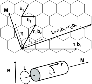
Figure 1: Upper: Lattice structure of the graphene sheet. The carbon atoms are located at the vertices of hexahedrons. $\overrightarrow{b}_{1}$ and $\overrightarrow{b}_{2}$ are primitive translation vectors. $\overrightarrow{L}$ is the chiral vector and $\overrightarrow{M}$ denotes the direction perpendicular to $\overrightarrow{L}$. The lengths of the vectors are $b=\sqrt{3}a_{C-C}$; $L=b\sqrt{n_{1}^{2}+n_{2}^{2}+n_{1}n_{2}}$; $a_{C-C}$ is the distance between the nearest carbon atoms. The figure depicts the particular case of $n_{1}=4$, $n_{2}=2$. Lower: CNT as a tortile graphene sheet. $\xi$ and $\eta$ denote the coordinates for the electronic states. The direction of the magnetic field $\overrightarrow{B}$ is also shown.

where $A_{0}$ denotes the length of the CNT, $\vec{L}$ ($=n_{1}\overrightarrow{b}_{1}+n_{2}\overrightarrow{b}_{2}$) the chiral vector in terms of primitive translation vectors $\overrightarrow{b}_{1}$, $\overrightarrow{b}_{2}$ and integers $n_{1}$, $n_{2}$, and $B_{\nu,n}(k)=[$æ${}_{\nu,n}-ik]/\sqrt{\text{\ae}_{\nu,n}{}^{2}+k^{2}}$ with æ${}_{\nu,n}=(2\pi/L)(n-\nu/3)$; the quantum number $n=0,\pm 1,\pm 2,...$ distinguishes the energy bands, while $\nu$ takes one of the three integers $-1,0,1$ that makes $(n_{1}-n_{2}-\nu)$ an integer multiple of $3$. As shown in Fig. 1, $\xi$ and $\eta$ represent the coordinates for the axes directed along $\overrightarrow{L}$ (i.e., the circumference) and the CNT (i.e., $\overrightarrow{M}$), respectively. The eigenstates $\left|k^{\prime}\right\rangle$ for the $K^{\prime}$ valley can be readily obtained from Eq. (2) by substituting $B_{\nu,n}\rightarrow B_{-\nu,n}^{\ast}$, and $k\rightarrow k_{\nu,n}^{\prime}$. The wave vectors $k$ and $k^{\prime}$ are determined from the $K$ and $K^{\prime}$ points of the Brillouin zone, respectively.

The corresponding dispersion relation for the $\left|k\right\rangle$ states reads

$$\varepsilon_{n,k}=\gamma\sqrt{\text{\ae}_{\nu,n}{}^{2}+k^{2}},$$ (3)

where $\gamma$ is a transfer matrix element. Assuming that only the lowest conduction band is occupied by electrons in a semiconducting CNT with $\nu=+1$ or $-1$, we restrict our consideration to the $n=0$ case at a given temperature $T$. Then, Eq. (3) in the vicinity of the $K$ point can be approximated as

$$\varepsilon_{k}=\frac{E_{g}}{2}+\frac{\hbar^{2}k^{2}}{2m^{\ast}}$$ (4)

with an effective mass $m^{\ast}=2\pi\hbar^{2}/3L\gamma$ and the band gap $E_{g}=4\pi\gamma/3L$. In the $K^{\prime}$ valley, a similar dispersion relation can be obtained when $k$ is substituted by $k^{\prime}$. Although it is known that the external magnetic field $\overrightarrow{B}$ modifies the CNT electronic states, this effect is neglected as the relevant parameter $(d_{t}/2a_{H})^{2}$ (where $d_{t}=|\vec{L}|/\pi$ is the CNT diameter and $a_{H}=\sqrt{c\hbar/eB}$ the magnetic length) is practically very small.Ando05 ; AjikiAndo Hence, we only consider the influence of $B$ on electron spin states through the Zeeman energy $\hbar\omega\sigma$; $\sigma=\pm 1/2$ is the spin projection on the $\overrightarrow{B}$ direction.

Utilizing the expressions given above, we can represent the fluctuating field operator in a second-quantized form in terms of the electron creation-annihilation operators $a_{k,\sigma}^{{\dagger}}$ and $a_{k,\sigma}$,

$$\Theta_{\mu}=\frac{a_{NT}}{A_{0}}\sum_{k_{1},k_{2},\sigma}\sum_{j=1}^{N}e^{i(k_{1}-k_{2})\eta_{j}}I_{\mu}^{j}a_{k_{1},\sigma}^{{\dagger}}a_{k_{2},\sigma},$$ (5)

where $\mu$ denotes the coordinate for the spin states; by convention, the direction of the magnetic field $\overrightarrow{B}$ is chosen as the $z$ axis (quantization axis) and two transversal directions as $x$ and $y$ ($\mu=x,y,z$). In addition, $a_{NT}=a_{hf}\Omega_{0}/L$ and $\eta_{j}$ is the location of the $j$-th nuclear spin on the CNT axis. As $k_{1}$ and $k_{2}$ are any two states in the Brillouin zone, Eq. (5) accounts for the effects of both intra- and inter-valley electron scattering on the nuclear spins.

Let us now consider the spin evolution caused by arbitrary random fluctuations $\Theta_{\mu}(t)$. The time dependence of the mean spin value $\vec{s}$ can be described by the quantum kinetic equation provided the spin relaxation times $T_{1}$ and $T_{2}$ are much longer than the correlation time of the thermal bath: Sem03

$$\frac{d}{dt}\vec{s}(t)=\vec{\omega}\times\vec{s}(t)-\mathbf{\Gamma}\left[\vec{s}(t)-\vec{s}_{0}\right],$$ (6)

where $\vec{\omega}=\omega\overrightarrow{B}/|\overrightarrow{B}|$ if the $g$-factor anisotropy is ignored and the electron spin polarization at thermal equilibrium $\vec{s}_{0}$ is given as $-{\frac{1}{2}}\widehat{z}\tanh(\hbar\omega/2k_{B}T)$ ($k_{B}$ the Boltzmann constant). Finally, the matrix $\mathbf{\Gamma}$ of the relaxation coefficients can be reduced to the Bloch-Redfield diagonal form with a leading diagonal composed of matrix elements $\Gamma_{xx}=T_{2}^{-1}$, $\Gamma_{yy}=T_{2}^{-1}$, and $\Gamma_{zz}=T_{1}^{-1}$:

$$T_{1}^{-1} = 2\pi n(\omega)\gamma_{xx}(\omega),$$ (7)

$$T_{2}^{-1} = \pi[\gamma_{zz}(0)+n(\omega)\gamma_{xx}(\omega)],$$ (8)

where $n(\omega)=(1+e^{-\hbar\omega/k_{B}T})/2$ and $\gamma_{\mu\mu}(\omega)$ is the Fourier transformed correlation function of the operator $\Theta_{\mu}$,

$$\gamma_{\mu\mu}(\omega)=\frac{1}{2\pi\hbar^{2}}\int_{-\infty}^{\infty}\left\langle\Theta_{\mu}(\tau)\Theta_{\mu}\right\rangle e^{i\omega\tau}d\tau.$$ (9)

Hence, evaluation of the longitudinal $T_{1}$ and the transversal $T_{2}$ relaxation times can be reduced to finding the relevant $\gamma_{\mu\mu}$. In Eq. (9), $\Theta_{\mu}\left(\tau\right)=\exp(iH_{d}\tau/\hbar)\Theta_{\mu}\exp(-iH_{d}\tau/\hbar)$, $\left\langle\ldots\right\rangle=Tr\{e^{-H_{d}/k_{B}T}\ldots\}/Tre^{-H_{d}/k_{B}T}$, where $H_{d}$ is the Hamiltonian of the thermal bath. In our case, it takes the form

$$H_{d}=\sum\limits_{\mathbf{k},\sigma}\varepsilon_{\mathbf{k}}a_{\mathbf{k},\sigma}^{\dagger}a_{\mathbf{k},\sigma}+\sum_{j}\hbar\omega_{n}I_{Z}^{j}.$$ (10)

The first term of Eq. (10) represents the kinetic energy of the electron, which is basically the electron Hamiltonian after the Zeeman energy $\sum\limits_{\mathbf{k},\sigma}\hbar\omega\sigma a_{\mathbf{k},\sigma}^{\dagger}a_{\mathbf{k},\sigma}$ is removed; as defined earlier, $a_{\mathbf{k},\sigma}^{\dagger}$ and $a_{\mathbf{k},\sigma}$ are the creation and annihilation operators of an electron with energy $\varepsilon_{\mathbf{k}}$ [Eq. (4)] and $\sigma$ is the electron spin quantum number. The second term accounts for the magnetic energy due to the nuclear spin splitting $\hbar\omega_{n}$ in a magnetic field.

As the electron momentum relaxation time $\tau_{k}$ is expected to be shorter than the spin relaxation time, the correlation functions can be found from Eq. (9) in terms of $\delta$-functions reflecting conservation of energy, when the average electron kinetic energy $\left\langle\varepsilon_{\mathbf{k}}\right\rangle\approx k_{B}T$ is much larger than the energy broadening $\Gamma$ of the order of $h\tau_{k}^{-1}$ (i.e., $k_{B}T\gg h\tau_{k}^{-1})$. To further simply the formulation, the nuclear spin operator $I_{x}$ contained in the fluctuating field operator $\Theta_{x}$ [Eq. (5)] is conveniently split into two parts $I_{x}=(I_{+}+I_{-})/2$ with the raising and lowering operators $I_{\pm}=I_{x}\pm iI_{y}$; correspondingly, $\Theta_{\pm}$ is defined from $\Theta_{x}=(\Theta_{+}+\Theta_{-})/2$ as a formal substitution for index $\mu$. Then, by averaging $e^{i(k_{1}-k_{2})\eta_{j}}$ over the random distribution of $N$ nuclear isotopes ¹³C, the Fourier transformation $\gamma_{\pm\mp}\left(\omega\right)$ of the correlation function $\left\langle\Theta_{\pm}(\tau)\Theta_{\mp}\right\rangle$ gives

$$\gamma_{\pm\mp}\left(\omega\right)=2N\frac{a_{NT}^{2}}{\hbar A_{0}^{2}}\left\langle I_{\pm}I_{\mp}\right\rangle\sum\limits_{k,k,\sigma}f_{k,\sigma}(1-f_{k^{\prime},\sigma})\delta\left(\pm\hbar\omega_{n}+\varepsilon_{k}-\varepsilon_{k^{\prime}}+\hbar\omega\right).$$ (11)

The distribution function $f_{k,\sigma}=\left\langle a_{k,\sigma}^{{\dagger}}a_{k,\sigma}\right\rangle$ for non-degenerate electrons is $e^{-u_{k,\sigma}/k_{B}T}/\sum_{k,\sigma}e^{-u_{k,\sigma}/k_{B}T}$, where $u_{k,\sigma}=u_{k}+\hbar\omega\sigma$, $u_{k}=\varepsilon_{k}-E_{g}/2$. Since $\gamma_{++}(\omega)=\gamma_{--}(\omega)=0$ from $\left\langle I_{+}I_{+}\right\rangle=\left\langle I_{-}I_{-}\right\rangle=0$, Eq. (11) allows one to find $\gamma_{xx}(\omega)=\left[\gamma_{+-}(\omega)+\gamma_{-+}(\omega)\right]/4$ as well as $n(\omega)\gamma_{xx}(\omega)$ in the form

$$n(\omega)\gamma_{xx}(\omega)=\frac{1}{8}\left[\gamma_{+-}(\omega)+\gamma_{-+}(\omega)+\gamma_{+-}(-\omega)+\gamma_{-+}(-\omega)\right].$$ (12)

Using Eqs. (11) and (12) and identity $\left\langle I_{\pm}I_{\mp}\right\rangle=\left\langle I_{x}^{2}\right\rangle+\left\langle I_{y}^{2}\right\rangle\pm\left\langle I_{z}\right\rangle\cong 2\left\langle I_{x}^{2}\right\rangle$, one can derive relaxation parameters in Eqs. (7) and (8). Under the assumption that the nuclear spin splitting $\omega_{n}$ is negligible compared to $\omega$, it takes the form

$$\pi n(\omega)\gamma_{xx}(\omega)=N\frac{a_{NT}^{2}}{\hbar A_{0}^{2}}\sum_{k,k^{\prime},\sigma}\left\langle I_{x}^{2}\right\rangle\left[f(1-f^{\prime})+f^{\prime}(1-f)\right]\left[\delta\left(\hbar\omega+\varepsilon-\varepsilon^{\prime}\right)\right],$$ (13)

where $\varepsilon=\varepsilon_{k,\sigma}$, $\varepsilon^{\prime}=\varepsilon_{k^{\prime},\sigma}$. Applying inequalities $f=f_{k,\sigma}\ll 1$, $f^{\prime}=f_{k^{\prime},\sigma}\ll 1$, Eq. (13) for non-degenerate electrons reduces to

$$\pi n(\omega)\gamma_{xx}(\omega)=2N\frac{a_{NT}^{2}}{\hbar A_{0}^{2}}\left\langle I_{x}^{2}\right\rangle\sum_{k,k^{\prime},\sigma}f_{k,\sigma}\delta(\hbar\omega+\varepsilon_{k}-\varepsilon_{k^{\prime}}).$$ (14)

Similarly, we find

$$\pi\gamma_{zz}(0)=2N\frac{a_{NT}^{2}}{\hbar A_{0}^{2}}\left\langle I_{z}^{2}\right\rangle\sum_{k,k\mathbf{{}^{\prime}},\sigma}f_{k,\sigma}\delta(\varepsilon_{k}-\varepsilon_{k^{\prime}}).$$ (15)

Note that in the case of $I=1/2$, $I_{\mu}^{2}=\frac{1}{2}\widehat{\mathbf{1}}$ that leads to $\left\langle I_{x}^{2}\right\rangle=\left\langle I_{z}^{2}\right\rangle=1/4$ ($\widehat{\mathbf{1}}$ is the unity matrix).

One can see that the contribution of the elastic scattering that does not involve electron and nuclear spin flip-flop [Eq. (15)] differs from that of the inelastic process [Eq. (14)] by $\hbar\omega$ in the argument of the $\delta$-function. Subsequently, we focus on the calculation of $\gamma_{xx}(\omega)$ that covers the case of Eq. (15) in the limit $\omega\rightarrow 0$. The sum over the wave vectors in Eqs. (14) and (15) can be calculated by integrating the energy $u=\varepsilon_{k}-E_{g}/2$ with the density of states $D(u)$. In the vicinity of each valley,

$$D(u)=\frac{A_{0}}{\pi\hbar}\sqrt{\frac{2m^{\ast}}{u}}$$ (16)

that leads to the electron distribution function in the form

$$\sum_{\sigma}f_{k,\sigma}=\frac{\hbar}{2A_{0}}\sqrt{\frac{2\pi}{m^{\ast}k_{B}T}}e^{-u_{k}/k_{B}T}.$$ (17)

It can be shown that the double summation over $k$ and $k^{\prime}$ can be reduced to the summation over a single valley by multiplying the result by the valley degeneracy $l_{v}=2$. Straightforward calculation of the integrals with the density of states $D(u)$ under the condition $\hbar\omega\ll k_{B}T$ results in

$$n(\omega)\gamma_{xx}(\omega)=\frac{a_{NT}^{2}l_{v}\sqrt{m^{\ast}}}{\pi\hbar^{2}\sqrt{2\pi k_{B}T}}\frac{N}{A_{0}}\ln\frac{k_{B}T}{\hbar\omega}.$$ (18)

In the limit $\omega\rightarrow 0$, Eq. (18) reveals a logarithmic singularity. This situation is not only typical for one-dimensional systems but also known in the galvanomagnetic effect in bulk crystals. A standard recipe for removing such a divergency consists of taking into account broadening of the energy levels $\Gamma$ due to the electron scattering processes discussed earlier. Therefore, as soon as $\hbar\omega$ becomes smaller than this broadening factor $\Gamma$, the magnetic field dependence becomes saturated at $\ln(k_{B}T/\Gamma)$ instead of $\ln(k_{B}T/\hbar\omega)$ in Eq. (18). Moreover, one must also take into account the finite length $A_{0}$ of an actual CNT. In such a case, the electron energy cannot be less than $\Delta\varepsilon\approx\hbar^{2}/m^{\ast}A_{0}^{2}$, which substitutes $\Gamma$ if $\Delta\varepsilon>\Gamma$. In the following, we assume that the effect of finite $\Delta\varepsilon$ is included in the parameter $\Gamma$. Note that a similar restriction on the bottom limit of the electron energy $u$ would be applied to $D(u)$ in Eq. (16). Therefore the condition for the validity of Eq. (18) will be satisfied by $\max\{\Gamma,\hbar\omega\}\ll k_{B}T$.

In a manner similar to that discuss above, we can find $\gamma_{zz}(0)$, which looks like Eq. (18) with $\hbar\omega\rightarrow\Gamma$. The final expressions for relaxation times [Eqs. (7) and (8)] take the form

$$T_{1}^{-1} = \tau_{hf}^{-1}\ln\frac{k_{B}T}{\max\{\hbar\omega,\Gamma\}},$$ (19)

$$T_{2}^{-1} = \frac{\tau_{hf}^{-1}}{2}\left(\ln\frac{k_{B}T}{\Gamma}+\ln\frac{k_{B}T}{\max\{\hbar\omega,\Gamma\}}\right),$$ (20)

where the essential part, which determines the order of magnitude of the spin relaxation, can be expressed in terms of the fundamental CNT parameters

$$\tau_{hf}^{-1}=\frac{2l_{v}xa_{hf}^{2}\Omega_{0}}{\hbar\sqrt{3\gamma L^{3}k_{B}T}}.$$ (21)

Equations (19), (20) and (21) exhibit an unusual temperature dependence for the spin relaxation rate; in contrast to the three-dimensional case, decreasing $T$ enhances spin relaxation. Apparently, this effect stems from the property of the one-dimensional density of states, which increases as $u$ decreases to $\Gamma$. Equation (21) also shows that the geometric properties of different CNTs manifest itself only via the length of the chirality vector as a factor $L^{-3/2}$ ($L=\left|\overrightarrow{b}_{1}\right|\sqrt{n_{1}^{2}+n_{2}^{2}+n_{1}n_{2}}$). Hence, the relaxation rates for a variety of semiconducting CNTs can be readily compared by using this scaling rule. As for the magnetic field dependence, it appears in Eqs. (19) and (20) as the parameter $\hbar\omega$, which interplays with $\Gamma$. When $\hbar\omega>\Gamma$, the calculation predicts gradual reduction of the spin relaxation rate as $B$ increases. On the other hand, no magnetic field influence can be expected once $\hbar\omega$ drops below $\Gamma$.

As an example, we consider a zigzag CNT with $(n_{1},n_{2})=(8,0)$ and assume $\Gamma=1$ $\mu$eV. Other parameters are known to be: $x=0.011$, $\Omega_{0}=\sqrt{3}b^{2}/4$, $b=0.249$ nm, $\gamma=\gamma_{0}\Omega_{0}/b$, $\gamma_{0}=3.013$ eV. Dresselhaus The HFI constant for ¹³C was estimated in Ref. Barone, : $a_{hf}/2\pi\hbar=22.5$ MHz. Figure 2 presents the calculated relaxation rates $T_{1}^{-1}$ and $T_{2}^{-1}$ as a function of temperature at various magnetic field strengths. Clearly, spin relaxation becomes slower with the increasing temperature as discussed above. $T_{1}$ is always longer than $T_{2}$ with the exception of the zero-field case, where the longitudinal and transversal relaxations are indistinguishable. Both relaxation rates also show gradual decrease as $B$ becomes larger. With the relaxation time of about 1 s, these characteristics are readily observable by experiments.

In order to consider the effect of radial confinement, we calculate the spin-flip rate $W_{d}$ in bulk diamond. In general, $W_{d}=n\overline{v}\sigma_{sf}$, where $n=2x/\Omega_{d}$ is the nuclear spin concentration ($\Omega_{d}$ is the unit cell volume of diamond), $\overline{v}=\sqrt{8k_{B}T/\pi m}$ the mean electron velocity at temperature $T$, and $m=\sqrt[3]{m_{\shortparallel}m_{\perp}^{2}}$ the density of states effective mass. $m_{\shortparallel}$ and $m_{\perp}$ are the longitudinal and transversal masses in each of diamond $X$ valleys with six fold degeneracy (i.e., $l_{v}=6$). The spin-flip cross section for electron scattering with a localized spin moment calculated in the first Born approximation is known to be $\sigma_{sf}=\frac{2}{3\pi\hbar^{4}}I(I+1)l_{v}a_{hf}^{2}\Omega_{d}^{2}m^{2}$ [see Ref. Deigen, ]. Taking into account that $\Omega_{d}=5.67\times 10^{-24}$ cm³, $m_{\shortparallel}=1.4m_{0}$ and $m_{\perp}=0.36m_{0}$ ($m_{0}$ is the free electron mass), one can estimate the spin-flip relaxation time $W_{d}^{-1}=4.7\times 10^{3}$ s. This value exceeds the CNT relaxation time at $T=4$ K and $B=0$ by at least of four orders of magnitude, demonstrating the significance of the radial confinement effect in a CNT.

In conclusion, we consider electron spin relaxation in a single-walled semiconducting CNT through the HFI with nuclear spins of ¹³C isotopes. The analysis reveals the peculiarities in spin relaxation inherent to one dimensional systems at low temperatures and/or weak magnetic fields. As a result, it becomes dependent on the non-magnetic electron scattering. Numerical estimations illustrate the relative importance of this relaxation mechanism in a CNT compared to the similar processes in bulk diamond and other carbon-based structures; strong enhancement due to the radial confinement of electrons helps making the HFI dominant over the spin-orbital interactions, particularly at weak magnetic fields and low temperatures. However, the anticipated spin relaxation time of the order of 1 s in CNTs is still much longer than those found in conventional semiconductor structures.

This work was supported in part by the SRC/MARCO Center on FENA and US Army Research Office.

Figure 2: Calculated spin relaxation rates (a) $T_{1}^{-1}$ and (b) $T_{2}^{-1}$ in a (8,0) zigzag CNT as a function of temperature for different values of magnetic field $B$. The strength of the magnetic field is indicated in units of Tesla.

References

(1) See, for example, C. Dekker, Phys. Today 52, 22
(1999); T. W. Odom, J. L. Huang, P. Kim, and C. M. Lieber, J. Phys. Chem. B
104, 2794 (2000).
(2)Carbon Nanotubes: Synthesis, Structure,
Properties and Applications, ed. M. S. Dresselhaus, G. Dresselhaus, and P.
Avouris (Springer, Berlin, 2000); M. S. Dresselhaus, G. Dresselhaus, and P.
S. Eklund, Science of Fullerences and Carnon Nanotubs (Academic,
New York. 1996).
(3) T. Ando, J. Phys. Soc. Japan 74, 777 (2005).
(4) K. Tsukagoshi, B. W. Alphenaar, and H. Ago, Nature
401, 572 (1999).
(5) S. Sahoo, T. Kontos, and C. Schönenberger, Appl. Phys.
Lett. 86, 112109 (2005).
(6) H. Mehrez, J. Yaylor, H. Guo, J. Wang, and C. Roland, Phys.
Rev. Lett. 84, 2682 (2000).
(7) C.-K. Yang, J. Zhao, and J. P. Lu, Phys. Rev. Lett. 90, 257203 (2003).
(8) A. De Martino, R. Egger, K. Hallberg, and C. A.
Balseiro, Phys. Rev. Lett. 88, 206402 (2002).
(9) A. De Martino, R. Egger, F. Murphy-Armando, and K.
Hallberg, J. Phys.: Condens. Matter 16, S1437 (2004).
(10) T. Ando, J. Phys. Soc. Japan 69, 1757 (2000).
(11) H. Ajiki and T. Ando, J. Phys. Soc. Japan 62,
1255 (1993).
(12) Y. G. Semenov, Phys. Rev. B 67, 115319 (2003).
(13) T. Ando and K. Akimoto, J. Phys. Soc. Japan 73,
1895 (2004).
(14) V. Barone, J. Chem. Phys. 101, 6834 (1994).
(15) M. F. Deigen, V. S. Vikhnin, Yu. G. Semenov, and B. D.
Shanina, Fiz. Tverd. Tela 18, 2222 (1976) [Sov. Phys. Solid State
18, 1293 (1976)].