Self-organization with equilibration:
a model for the intermediate phase in rigidity percolation

Abstract

Recent experimental results for covalent glasses suggest the existence of an intermediate phase attributed to the self-organization of the glass network resulting from the tendency to minimize its internal stress. However, the exact nature of this experimentally measured phase remains unclear. We modify a previously proposed model of self-organization by generating a uniform sampling of stress-free networks. In our model, studied on a diluted triangular lattice, an unusual intermediate phase appears, in which both rigid and floppy networks have a chance to occur, a result also observed in a related model on a Bethe lattice by Barré et al. [Phys. Rev. Lett. 94, 208701 (2005)]. Our results for the bond-configurational entropy of self-organized networks, which turns out to be only about 2% lower than that of random networks, suggest that a self-organized intermediate phase could be common in systems near the rigidity percolation threshold.

I Introduction

Rigidity theory Thorpe (1983); Feng and Sen (1984); Jacobs and Thorpe (1995); Moukarzel and Duxbury (1995); Thorpe et al. (1999) has improved considerably our understanding of the structural, elastic and dynamical properties of systems such as chalcogenide glasses Thorpe (1983); Thorpe et al. (1999); Boolchand et al. (1999), interfaces Lucovsky et al. (1999) and proteins Rader et al. (2002), as a function of their connectivity. In its classical version, it introduces the concept of a rigidity transition, separating a soft (or floppy) and a rigid phases characterized by a mean coordination number. In many systems, optima or thresholds of various physical quantities are often observed at the rigidity transition. Some time ago, for example, Phillips Phillips (1979) noted that among chalcogenides, the best glassformers have a mean coordination such that the number of degrees of freedom is equal to the number of covalent (bond-stretching and bond-bending) constraints. At this point, corresponding to the rigidity transition, networks are largely rigid but stress-free. This prevents crystallization for both kinetic and thermodynamic reasons: being stress-free, the glassy state is not too energetically unfavorable compared to the crystal; being rigid, the networks lack the flexibility to efficiently explore the phase space and reach the crystalline state fast. Similarly, in the last 5 years, it has become clear that most proteins in their native state sit almost exactly at the rigidity transition, which could be necessary to have enough flexibility to fullfill their function while retaining their overall structure Rader et al. (2002).

Recently, a series of experiments on chalcogenide and oxide glasses Selvanathan et al. (1999, 2000); Georgiev et al. (2000); Wang et al. (2000); Boolchand et al. (2001, 2002); Georgiev et al. (2003); Christova et al. (2003); Vempati and Boolchand (2004); Trachenko et al. (2004); Chakravarty et al. (2005); Černošková et al. (2005); Qu and Boolchand (2005); Wang et al. (2005); Vaills et al. (2005); Sharma et al. (2005) have demonstrated the existence of a number of interesting and surprising behaviors. For instance, glasses with nearly optimal properties, such as the absence of aging Vempati and Boolchand (2004); Chakravarty et al. (2005); Qu and Boolchand (2005) and vanishing non-reversing enthalpy of the glass transition Selvanathan et al. (1999, 2000); Georgiev et al. (2000); Wang et al. (2000); Boolchand et al. (2002); Georgiev et al. (2003); Vempati and Boolchand (2004); Chakravarty et al. (2005); Černošková et al. (2005); Qu and Boolchand (2005) are observed not just at a particular mean coordination, but in some range of coordinations, suggesting the presence of an intermediate phase between the floppy and the rigid phases. While the details and exact origin of this intermediate phase are still a matter of debate (see, for example, the recent experimental paper by Golovchak et al. Golovchak et al. (2006)), it appears that it is due to the self-organization of the network minimizing the internal stress. If, according to Phillips’ argument, we expect “optimal” glasses to be rigid but stress-free, we should now expect to find this property everywhere in the intermediate phase rather than only at a single critical point, as in the standard phase diagram of rigidity percolation; there is now some direct evidence for this Christova et al. (2003); Wang et al. (2005).

A few models were proposed to explain this self-organization. Thorpe et al. Thorpe et al. (2000); Thorpe and Chubynsky (2001) have shown in an out-of-equilibrium model that it is possible to generate a stress-free intermediate phase. Barré et al. Barré et al. (2005) have shown in addition that such a phase was thermodynamically stable on a ring-free Bethe lattice, where each site has 3 degrees of freedom, but the whole network is embedded in an infinite-dimensional space. Taking a different approach, Micoulaut Micoulaut (2002) demonstrated that one could recover an intermediate phase by concentrating all the strain in local structures.

The goal of this paper is to assess whether or not a self-organized network with a finite-dimensional topology is also thermodynamically possible. This verification is important on two counts: (1) the Bethe lattice is a loopless structure producing a first-order rigidity transition Moukarzel et al. (1997); Duxbury et al. (1999); Thorpe et al. (1999) while 2- and 3-dimensional regular networks undergo a second-order phase transition Jacobs and Thorpe (1995); Thorpe et al. (1999); (2) the original model of Thorpe et al. is an out-of-equilibrium model which could lead to highly atypical networks.

For simplicity, we study two-dimensional central-force (2D CF) networks. This allows us to consider networks of much bigger linear dimensions than is possible in 3D, limiting the finite-size effects. Moreover, in all cases studied until now, rigidity results for 2D CF networks have been qualitatively very similar to those obtained for 3D glass networks. Our results should therefore also apply to glass networks.

In the next section, we review the basic facts about rigidity and the intermediate phase. We then explain the model used here and present our results for a bond-diluted two-dimensional triangular network. We first discuss an unusual property of our model: a network in the intermediate phase can be either rigid or floppy with a finite probability. We then focus on the calculation of the entropy of self-organized networks.

II The intermediate phase in the rigidity phase diagram

In rigidity theory, an elastic network is characterized by the number of motions, called floppy modes, that do not distort any constraints. In a system with no constraints, all degrees of freedom are floppy modes and thus their number is $dN$, where $N$ is the number of atoms and $d$ is the dimensionality of space. In an approximation due to Maxwell and known as Maxwell counting Maxwell (1864), it is assumed that each additional constraint removes a floppy mode, so that the number of floppy modes for a given number of constraints $N_{c}$ can be written as

$$F=dN-N_{c}.$$ (1)

When the number of constraints becomes equal to the number of degrees of freedom, $F=0$ and the network undergoes a rigidity percolation transition, going from floppy to rigid. In a 2D CF network, the number of constraints per atom is $\langle r\rangle/2$, where $\langle r\rangle$ is the mean coordination (the average number of connections of a site); the critical coordination is therefore $\langle r\rangle=4$. In chalcogenide glasses, characterized by the chemical formula A_xB_yC_1-x-y, where A is an atom of valence 4 (usually Ge or Si), B is an atom of valence 3 (As or P) and C is a chalcogen (Se, S or Te), counting both covalent bonds and their related angular constraints, the critical coordination is $\langle r\rangle=2.4$ Thorpe (1983).

Since Maxwell counting is a mean-field theory, it ignores fluctuations and correlations that can be built in the network. An overall rigid network can have some internal localized floppy modes. Also, a constraint inserted into a piece of the network that is already rigid does not remove floppy modes. Such constraints, known as redundant, are obviously present in the rigid phase, where Eq. (1) gives a negative number of floppy modes, since this number cannot be lower than $d(d+1)/2$ (6 in 3D, 3 in 2D), to account for rigid body translations and rotations; but redundant constraints can also be present, of course, in an overall floppy network. In generic networks, such as glasses, where the bond lengths vary, these constraints create an internal stress and increase the elastic energy, since at least some part of the network has to be deformed to accommodate them.

If the number of redundant constraints, $N_{R}$, is known, then the Maxwell counting formula can be corrected:

$$F=dN-N_{c}+N_{R}.$$ (2)

This result is exact — the problem lies in calculating $N_{R}$. A theorem by Laman Laman (1970) makes this possible. Consider all possible subnetworks of a system. If the number of degrees of freedom minus the number of constraints is less than $d(d+1)/2$ for at least one subnetwork, there must be redundant constraints. Laman showed that this is the only way redundant constraints can occur: for them to be present, the above must be satisfied for at least one subnetwork. This is strictly true in 2D; although there are known counterexamples for general networks in 3D, it is assumed true (there is no rigorous mathematical proof, but no known counterexamples either) for glassy networks with covalent bonding including angular constraints Tay and Whiteley (1984); Whiteley (1999).

Laman’s theorem is used in a computer algorithm for rigidity analysis, known as the pebble game Jacobs and Thorpe (1995); Jacobs and Hendrickson (1997); Jacobs (1998); Jacobs et al. (1999, 2001). The pebble game starts with an empty network and then one constraint is added at a time and each added constraint is checked for redundancy. Thus at every stage in the network-building process the number of redundant constraints, $N_{R}$, and, according to Eq. 2, $F$, are known exactly. Independent constraints are matched to pebbles that are assigned to sites and whose total number is equal to the number of degrees of freedom; thus the number of free pebbles (not matched to any constraint) gives the number of floppy modes. The pebble game, in addition, identifies stressed regions in the network and also offers rigid cluster decomposition that identifies all rigid clusters in the network. The analysis provided by the pebble game is purely topological, the details of the geometry are not taken into account, nor is the exact expression for the forces. The downside is that the pebble game (as well as Laman’s theorem itself) is only applicable to generic networks: networks special in some way (having parallel bonds, for instance) may have rigidity properties that are different from those of the vast majority of networks of a given topology. The fraction of such special (or non-generic) networks among all networks of a given topology is, however, zero, and so a covalent glass network, being disordered, can be safely assumed to be generic.

Recently, a series of experiments Selvanathan et al. (1999, 2000); Georgiev et al. (2000); Wang et al. (2000); Boolchand et al. (2001, 2002); Georgiev et al. (2003); Christova et al. (2003); Vempati and Boolchand (2004); Chakravarty et al. (2005); Černošková et al. (2005); Qu and Boolchand (2005); Wang et al. (2005); Sharma et al. (2005) have suggested that there could be not one but two phase transitions near $\langle r\rangle=2.4$, with the opening of an intermediate phase between the phases already known. The properties of this phase suggest that the intermediate phase is rigid but stress-free. To explain the presence of two transitions and the intermediate phase between them within the framework of rigidity theory, it has been proposed Thorpe et al. (2000) that the glass networks self-organize in some way. Broadly speaking, any reduction in the amount of disorder in the network as it tries to minimize its free energy can be referred to as self-organization; chemical order, especially strong in oxide glasses like silica, would be one example. Thorpe et al. Thorpe et al. (2000); Thorpe and Chubynsky (2001) considered a particular kind of self-organization: glass networks minimizing their elastic stress energy. As a proof of principle, they constructed the following model. Starting with a low-coordination stress-free network, bonds are added one at a time with the restriction that they cannot be redundant and thus add stress to the network, using the pebble game for constructing and analyzing the network at each step. This process is repeated until it is no longer possible to add a bond without introducing stress to the network. After that, bond insertion continues at random. The maximum coordination at which no stress is present, according to Eq. (2), cannot exceed the rigidity threshold according to Maxwell counting ($\langle r\rangle=4$ for 2D CF networks and $\langle r\rangle=2.4$ for covalent glass networks). In fact, in the model of Thorpe et al., the Maxwell counting threshold value is reached without stress for 2D CF networks, but not for the 3D glass network Thorpe and Chubynsky (2001). In this model, once the stress appears, it immediately percolates, corresponding to the upper boundary of the intermediate phase. In general, this need not be the case, since a network can have finite stressed regions without stress percolating (this is the case in the model of Micoulaut and Phillips Micoulaut (2002); Micoulaut and Phillips (2003)).

To observe the rigidity transition in a two-dimensional diluted regular lattice, one needs a lattice with coordination bigger than 4, and so the triangular lattice is a natural choice. Since the pebble game algorithm can only be applied to generic networks, one has to assume that the triangular lattice is distorted (for example, by having some disorder in bond lengths). Previous numerical studies for the randomly diluted triangular lattice without self-organization indicate a single rigidity and stress transition at $\langle r\rangle=3.961$ — very close to the Maxwell counting prediction (Fig. 1) Jacobs and Thorpe (1995). Note that the rigidity and stress transitions coincide in this case.

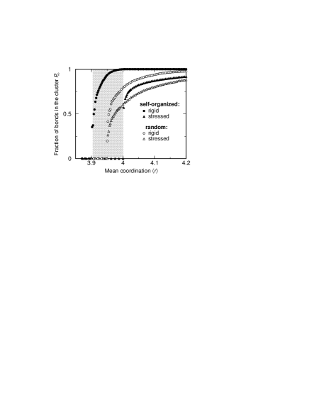
Figure 1: The dependence of the fraction of bonds in the percolating rigid cluster and the percolating stressed region for the random case and the self-organized case without equilibration. In the random case, the rigidity and stress percolation thresholds coincide. In the self-organized case, these thresholds do not coincide and there is an intermediate phase (shaded) between them. The stressed region is defined here as the contiguous percolating set of stressed bonds within the percolating rigid cluster. The simulations are averaged over 2 realizations on the bond-diluted triangular lattice of $400\times 400$ sites. The figure is taken from Ref. Thorpe and Chubynsky (2001).

In the self-organization model of Thorpe et al., a numerical simulation reveals instead two phase transitions (Fig. 1). As the coordination is increased from the floppy phase, a percolating rigid cluster appears at $\langle r\rangle=3.905$. At this point, by construction, the network is still stress-free. This is the lower boundary of the rigid but stress-free intermediate phase — the rigidity percolation transition. As the mean coordination continues to grow, keeping the network stress-free becomes impossible. At this point, which, as mentioned above, is at $\langle r\rangle=4$, the stress appears and immediately percolates. This is the stress percolation transition, which is the upper boundary of the intermediate phase.

The probability of a percolating cluster in the model of Thorpe et al. is zero below the rigidity percolation threshold and one above in the thermodynamic limit, as normally is the case for percolation transitions. This is illustrated in Fig. 2, where the probability of having a percolating cluster is shown for different network sizes. As expected, the dependence gets closer to a step function as the size increases.

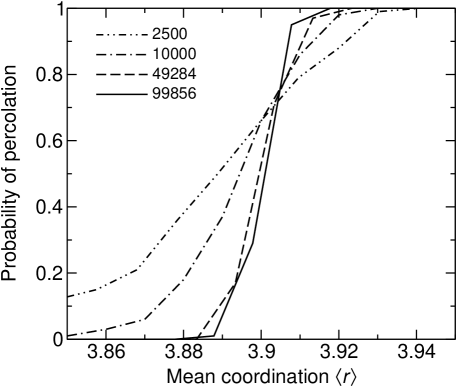
Figure 2: The fraction of networks in which the percolating rigid cluster is present as a function of $\langle r\rangle$ for the model of self-organization without equilibration. Each curve is obtained from 100 separate runs on a bond-diluted triangular lattice; the lattice sizes are indicated in the legend.

III A self-organization model with equilibration

The self-organization model of Thorpe et al. is peculiar in that bonds are only added to the network and never removed. While one can imagine a very rapid quench process in which indeed bond formation dominates, this process does not lead to formation of good glasses. Therefore a way of building equilibrated stress-free networks is needed. As the elastic energy of a stress-free network is zero, any such networks should occur with equal probability.

A similar issue arose before in the case of conventional (or connectivity) percolation. In the rigidity case, self-organization proceeds by avoiding stress or redundancy, i.e., bonds that connect already mutually rigid sites. The connectivity analog consists in avoiding connections between sites that are already connected, i.e., creating loops. Straley Straley (1979) proposed a model directly analogous to the one by Thorpe et al., i.e., with bonds inserted one at a time and those forming loops rejected; connectivity percolation occurs at some point, and then there is an “intermediate phase” (although it was not referred to as such in the connectivity percolation context) that is connected but without any loops, until a point is reached at which avoiding loops is no longer possible (at this point the network is a spanning tree). It was realized later on that this model does not produce a uniform ensemble, in which every loopless network would occur with equal probability. Several authors, using a variety of methods Wu (1978); Braswell et al. (1984); Straley (1990) , claimed then that in the equilibrated uniform ensemble, connectivity percolation does not occur until the spanning tree limit is reached, i.e., there is no intermediate phase. This shows that the results may change significantly depending on the ensemble of self-organized networks that is considered.

Braswell et al. Braswell et al. (1984), in particular, used the following algorithm to generate equiprobable loopless networks: take an arbitrary loopless network, choose a bond at random, delete it and then reinsert at an arbitrary place where it would not form a loop, with this place chosen equiprobably among all such places. They showed that after equilibration has taken place, this method would indeed generate the uniform ensemble of networks, by proving the detailed balance condition, i.e., that given some loopless network 1, the probability that in a single step of the algorithm some other network 2 would be produced is the same as the probability of going in the opposite direction, i.e., from network 2 to network 1. Their arguments fully apply to the rigidity case as well.

In view of the above, we consider a variety of the self-organization model by Thorpe et al., adding equilibration that produces equiprobable stress-free networks. Like in the previous model, we start with the “empty” network without bonds and start inserting bonds one by one without creating stress. After every bond insertion, we equilibrate by doing bond swaps following the procedure described above, i.e., choose a bond at random, delete it and then insert a bond elsewhere choosing at random among the places where that new bond would not create stress. It is worth noting that in general it is rather difficult to handle removal of constraints within the pebble game; but it is easy to remove an unstressed constraint, as this simply involves releasing the associated pebble with no additional pebble rearrangement. Since in our case all constraints are unstressed by construction, no problem arises. In this paper we focus on the intermediate phase and do not investigate the stressed phase, so we stop at the point at which further stressless insertion becomes impossible.

A very similar model has been proposed recently by Barré et al. Barré et al. (2005) using a Bethe lattice and, as an added sophistication, an energy-cost function linear in the number of redundant constraints. While this energy is somewhat unrealistic, it provides a thermodynamic justification for the existence of the intermediate phase. However, Bethe lattices are particular constructions, leading to a first-order rigidity phase transition while 2D central-force and 3D bond-bending networks show a second-order rigidity transition. By comparison, our model in essence assigns an infinite cost to redundant bonds and corresponds therefore to the $T\to 0$ limit of Barré’s model but on a regular lattice with a second-order rigidity transition.

IV Rigidity percolation in the intermediate phase

Our simulations for the new model with equilibration are done for 2D CF bond-diluted triangular lattices. Periodic boundary conditions were used with the supercell consisting of the same number of unit cells in both directions. We have chosen the duration of equilibration equal to 100 steps above $\langle r\rangle=3.5$ and 10 steps below (where even in random networks there are very few redundant constraints, so the self-organized networks are almost completely random anyway and long equilibration is not needed). This is sufficient for convergence as shown in Fig. 3 for a $100\times 100$ lattice; we also checked that 100 steps was sufficient by comparing with a very long equilibration run at a single point $\langle r\rangle=3.95$ for the largest lattice used here (not shown). The result we get is quite different from that obtained without equilibration. Fig. 4, just as Fig. 2, shows the probability of rigidity percolation as a function of $\langle r\rangle$ for several different sizes, but now for the model with equilibration. The self-organization still opens an intermediate phase around the critical point found at $\langle r\rangle\approx 3.961$ in the standard rigidity phase diagram. But rather than approaching a step function as the size increases, the result for the probability of percolation is now a gradual increase from 0 at $\langle r\rangle\approx 3.94$ to 1 at $\langle r\rangle=4$. This is similar to the result on a Bethe lattice in the model of Barré et al., even though the rigidity percolation transition is of a different order. The dependence of the percolation probability on $\langle r\rangle$ is close to linear and this linearity may, in fact, be exact, although a very small non-linear region near the lower boundary of the intermediate phase cannot be ruled out. One difference between our result and that presented by Barré et al. is that since their consideration is at a non-zero temperature, there is always a possibility of having a small number of redundant constraints; since adding very few (perhaps $\mathcal{O}(1)$) redundant constraints to an unstressed network is often enough for stress percolation, it is not surprising that they have found a finite probability of both rigidity and stress percolation in the intermediate phase, whereas in our case, the stress percolation probability is, of course, zero by construction.

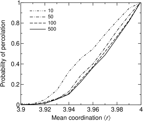
Figure 3: Same as in Fig. 2, but now for the model with equilibration, for triangular networks of 10000 sites and for several different equilibration times indicated in the legend as the number of equilibration steps per each inserted bond above $\langle r\rangle=3.5$; below $\langle r\rangle=3.5$, there are 10 equilibration steps per bond in all cases. The data are likewise from 100 separate runs, but in addition, from each run all networks obtained during the equilibration procedure at the given mean coordination are taken into account.

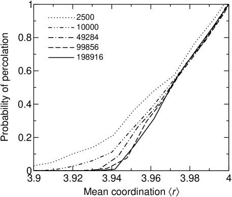
Figure 4: Same as in Fig. 3, but for different network sizes indicated in the legend, always using 10 equilibration steps per inserted bond below $\langle r\rangle=3.5$ and 100 equilibration steps above.

V Entropy cost of self-organization

Although we do not include a potential energy explicitly, the self-organization models discussed here are constructed to prevent the build-up of stress, implicitly minimizing the potential energy of the system. At a finite temperature, however, we are interested in minimizing the free energy. As glasses are formed at a non-zero temperature, the thermodynamical state will be influenced by the balance between the entropic cost associated with generating a self-organized network and the energetic cost of creating internal stress: if the entropy of the random network is large compared with that of the self-organized one, then it is likely that very little self-organization will take place and the problem discussed here becomes irrelevant.

The entropy of a covalent network can be viewed as consisting of two parts. The first part, the topological entropy, is proportional to the logarithm of the number of different possible bond topologies or bond configurations. The second part, which can be called, somewhat simplistically, the flexibility entropy, depends on the phase space available to each such bond configuration. This division of the total entropy is similar, but not identical, to the traditional division into the configurational and vibrational entropy in the inherent structure formalism Stillinger and Weber (1982). In particular, flexible networks exhibit a wide range of motions and would generally correspond to more than one inherent structure, when a potential energy function is defined. For this reason, the flexibility entropy includes both harmonic and anharmonic contributions associated with a given topology of the covalent network; its exact evaluation is difficult and goes beyond the scope of this paper. However, since the flexibility entropy is expected to be roughly proportional to the number of floppy modes Jacobs et al. (2003); Naumis (2005); Thorpe , and, according to Eq. (2), the number of floppy modes in a self-organized network (with $N_{R}=0$) is smaller than in a random network ($N_{R}>0$) with the same number of constraints $N_{c}$, the flexibility entropy of the self-organized network is likely to be smaller than that of the random network. This difference is probably not very large, especially in real systems where long-range forces reduce significantly the available configuration space even in the floppy phase.

The topological entropy is, in general, difficult to calculate as well, although methods, such as that by Vink and Barkema Vink and Barkema (2002), exist. It is much simpler for a lattice-based model like ours, as it requires only counting the number of possible bond configurations on a lattice. In this case, the topological entropy (which we can also call the bond-configurational entropy) is simply

$$S_{\rm bc}(\langle r\rangle)=\ln N_{\rm bc}(\langle r\rangle),$$ (3)

where $N_{\rm bc}(\langle r\rangle)$ is the number of stress-free configurations with mean coordination $\langle r\rangle$ and the Boltzmann constant $k_{B}$ is put equal to 1. To calculate $N_{\rm bc}$, we use the following approach. Suppose the number of stress-free networks having $N_{B}$ bonds, $N_{\rm bc}(N_{B})$, is known. From a stress-free network having $N_{B}$ bonds, it is possible to produce a stress-free network having $N_{B}+1$ bonds by adding a bond in one of those places where this added bond would not create stress. Suppose on average there are $n_{+}(N_{B})$ such places or ways to create a stress-free network with $N_{B}+1$ bonds. On the other hand, for any stress-free network with $N_{B}+1$ bonds, there are always exactly $n_{-}(N_{B}+1)=N_{B}+1$ ways of creating a stress-free network with $N_{B}$ bonds by removing any one of the $N_{B}+1$ bonds. Moreover, if a network with $N_{B}+1$ bonds can be created from a network with $N_{B}$ bonds by adding a bond, then the latter network can always be obtained from the former by removing that same bond and vice versa, so the process is reversible. Then the number of stress-free networks with $N_{B}+1$ bonds is

$$N_{\rm bc}(N_{B}+1) = N_{\rm bc}(N_{B})\cdot\frac{n_{+}(N_{B})}{n_{-}(N_{B}+1)}$$ (4)

$$= N_{\rm bc}(N_{B})\cdot\frac{n_{+}(N_{B})}{N_{B}+1}.$$

If $n_{+}(N_{B})$ is known for all $N_{B}$, then, using $N_{\rm bc}(0)=1$ as the initial condition, Eq. (4) can be iterated to yield all $N_{\rm bc}(N_{B})$. In practice, $n_{+}(N_{B})$ are obtained numerically, by a sort of Monte Carlo procedure, where some of the places in the network where a bond is missing (compared to the full undiluted lattice) are tried and it is found in what fraction of such places addition of a bond would not create stress. In our simulations, we use 100 such attempts per network. The result is then averaged over the networks with a given number of bonds obtained during the equilibration procedure.

Note that the same procedure can be repeated for the random case (without any self-organization). In this case, $n_{+}(N_{B})$ should count all ways to create a new network of $N_{B}+1$ bonds (no matter stress-free or not) out of a network of $N_{B}$ bonds, and there are as many ways to do that as there are places where a bond is missing (compared to the full lattice); thus for a random network, $n_{+}^{r}(N_{B})=N_{Bf}-N_{B}$, where $N_{Bf}$ is the number of bonds in the full lattice. On the other hand, the analog of quantity $n_{-}(N_{B}+1)$, which we denote $n_{-}^{r}(N_{B}+1)$, is still $N_{B}+1$. Therefore, for the random network,

$$N_{\rm bc}^{r}(N_{B}+1) = N_{\rm bc}^{r}(N_{B})\cdot\frac{n_{+}^{r}(N_{B})}{n_{-}^{r}(N_{B}+1)}$$ (5)

$$= N_{\rm bc}^{r}(N_{B})\cdot\frac{N_{Bf}-N_{B}}{N_{B}+1}.$$

This can, of course, be used to obtain the analytical result for any $N_{B}$, which is simply a binomial coefficient. If we are interested in the difference $\Delta S$ between the entropies of the random and self-organized networks, this is simply

$$\Delta S(N_{B})=\ln\frac{N_{\rm bc}^{r}(N_{B})}{N_{\rm bc}(N_{B})}.$$ (6)

The change of this difference when a bond is added is

$$\Delta S(N_{B}+1)-\Delta S(N_{B})=$$ (7)

$$= \ln\left(\frac{N_{\rm bc}^{r}(N_{B}+1)}{N_{\rm bc}^{r}(N_{B})}\cdot\frac{N_{\rm bc}(N_{B})}{N_{\rm bc}(N_{B}+1)}\right)$$

$$= \ln\left(\frac{n_{+}^{r}(N_{B})}{N_{B}+1}\cdot\frac{N_{B}+1}{n_{+}(N_{B})}\right)$$

$$= -\ln\nu(N_{B}),$$

where $\nu(N_{B})=n_{+}(N_{B})/n_{+}^{r}(N_{B})$ is the average fraction of bonds whose insertion would not create stress among all missing bonds in the network. Note that $\nu(N_{B})$ is what is calculated directly by the Monte Carlo procedure described above.

The entropy $S$ is, of course, an extensive quantity, i.e., it is proportional to the network size (for big sizes). We can introduce the entropy per bond of the full lattice, $s=S/N_{Bf}$. In the thermodynamic limit,

$$\frac{{\rm d}(\Delta s)}{{\rm d}\langle r\rangle} = \frac{\Delta S(N_{B}+1)-\Delta S(N_{B})}{N_{Bf}\left[\langle r\rangle\Big{|}_{N_{B}+1}-\langle r\rangle\Big{|}_{N_{B}}\right]}$$ (8)

$$= -\frac{\ln\nu}{N_{Bf}\left[\langle r\rangle\Big{|}_{N_{B}+1}-\langle r\rangle\Big{|}_{N_{B}}\right]},$$

where $\langle r\rangle\Big{|}_{N_{B}}$ is the mean coordination of a network with $N_{B}$ bonds, and since $\langle r\rangle\Big{|}_{N_{B}}=2N_{B}/N$,

$$\frac{{\rm d}(\Delta s)}{{\rm d}\langle r\rangle}=-\frac{N}{2N_{Bf}}\ln\nu.$$ (9)

In the full triangular lattice, the number of bonds $N_{Bf}$ is three times the number of sites $N$, so we get

$$\frac{{\rm d}(\Delta s)}{{\rm d}\langle r\rangle}=-{1\over 6}\ln\nu.$$ (10)

The quantity $\nu$ obtained numerically is plotted in Fig. 5. From this plot, it seems to go to zero as $\delta=4-\langle r\rangle\to 0^{+}$ and appears to change linearly as a function of $\delta$ in this limit. In general, if in this limit $\nu\sim\delta^{m}$, then, according to Eq. (10),

$$s(\delta)={m\over 6}\delta\ln\delta+\text{regular\ part}.$$ (11)

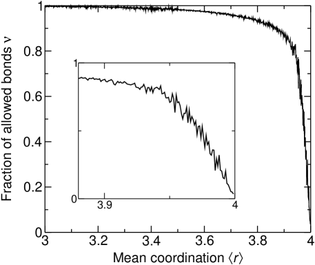
Figure 5: The fraction $\nu$ of “allowed bonds” (places where a bond can be inserted without creating stress) as a function of the mean coordination $\langle r\rangle$, for a triangular network of 50176 sites, with equilibration time of 1000 steps per inserted bond above $\langle r\rangle=3.5$ and 10 steps below. The result is obtained by a Monte Carlo procedure described in the text; at each mean coordination, it is averaged over the networks obtained during equilibration.

Figure 6 shows the entropy difference $\Delta s$ calculated by iterating Eq. (7), with $\nu$ obtained numerically after every bond addition. Since the simulations are done for networks of a finite size and with finite equilibration time, an extrapolation to the infinite size was done by fitting the simulation results to the function

$$\Delta s(\langle r\rangle;N,\tau)={A(\langle r\rangle)\over N}+{B(\langle r\rangle)\over\tau}+C(\langle r\rangle),$$ (12)

where $\tau$ is the equilibration time (in equilibration steps per added bond) used above $\langle r\rangle=3.5$ (below 3.5, we always use just 10 steps, for reasons explained above). As in different runs for different sizes the data were taken at slightly different points, linear interpolation was sometimes done to obtain the values at the same $\langle r\rangle$ in all cases. In total, data for 182 $(N,\tau)$ combinations were used, with $N$ between 5476 and 50176 sites and $\tau$ between 20 and 1000 steps (up to 10000 steps for 10000 sites). Data for higher $N$ and $\tau$ were assigned higher weights in the fit, since increasing $N$ and $\tau$ decreases the amount of noise in the data (the latter because the results for $\nu$ are averaged over all equilibration steps, and thus the more equilibration steps there are the smaller the error in $\nu$). Function $C(\langle r\rangle)$ representing the asymptotic value of the entropy difference is also shown in Fig. 6.

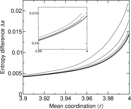
Figure 6: The difference in the bond-configurational entropy between random and self-organized triangular networks, $\Delta s$, as a function of the mean coordination $\langle r\rangle$, shown for several network sizes and equilibration times, as well as the asymptotic value (i.e., the extrapolation to the infinite size and relaxation time, as described in the text). Quantity $\nu$ used to calculate $\Delta s$ is obtained by the Monte Carlo procedure described in the text and then averaged over networks obtained during equilibration at the given $\langle r\rangle$. In the main plot, all thin lines are results for 50176 sites; the equilibration times are, top to bottom: 10 steps, 30 steps, 100 steps and 300 steps per added bond. The thick line is the asymptotic. In the inset, all thin lines are results for 1000 equilibration steps per added bond. The sizes are, top to bottom: 5476 sites, 15376 sites and 50176 sites. The thick line is again the asymptotic. The asymptotics are themselves extrapolated to $\langle r\rangle=4$, as described in the text. All equilibration times listed are for $\langle r\rangle>3.5$; for $\langle r\rangle<3.5$, 10 equilibration steps per added bond are always used.

For a finite-size network, it is only possible to reach a point 3 bonds short of $\langle r\rangle=4$ without creating stress. For this reason, our simulations were stopped somewhere around $\langle r\rangle=3.999$. Taking into account Eq. (11), we have fitted the asymptotic entropy difference $C(\delta)$ between $\langle r\rangle=3.97$ and 3.999 using the following function:

$$C(\delta)=a_{0}+a_{1}\delta\ln\delta+a_{2}\delta+a_{3}\delta^{2}.$$ (13)

The fit is essentially perfect, and the obtained value of $a_{1}=0.1636$ is consistent with the value of $1/6$ expected for $m=1$, according to Eq. (11). The fit is used to complete the curve in Fig. 6 up to $\langle r\rangle=4$. The value of the entropy difference at $\langle r\rangle=4$ is $a_{0}=0.0146$. This is the biggest value of the entropy difference, but it is still small, only about 2% of the bond-configurational entropy of the random network (which at $\langle r\rangle=4$, when 2/3 of the bonds are present, is $-[(2/3)\ln(2/3)+(1/3)\ln(1/3)]=0.6365\ldots$).

In the above calculation of the entropy we explicitly use the fact that all stress-free networks with a given number of bonds are equiprobable in our new model. A similar consideration for the old self-organization model without equilibration would be much more difficult.

We note, finally, that according to Eq. (11), there is a non-analyticity in the behavior of the entropy when $\langle r\rangle\to 4^{-}$, i.e., at the stress transition. We should also expect some very weak non-analyticity (perhaps a break or a cusp in a higher derivative) at the lower boundary of the intermediate phase (the rigidity transition) at $\langle r\rangle\approx 3.94$, but it is too weak to be seen in our simulation results.

VI Conclusion

We have considered a model of self-organization in elastic networks, adding an equilibration feature to the model previously considered by Thorpe et al. Thorpe et al. (2000); Thorpe and Chubynsky (2001). In our model, we find an intermediate phase in the rigidity phase diagram, in which the fraction of networks in which rigidity percolates is between 0 and 1 in the range of mean coordination between 3.94 and 4.0 for the bond-diluted triangular lattice, a result qualitatively similar to that obtained by Barré et al. Barré et al. (2005) in a closely related model on a Bethe lattice.

Calculating the bond-configurational entropy of these self-organized networks, we find that it is only about 2% smaller than that of randomly-connected networks. Provided that the flexibility entropy, which should reduce the stability of the intermediate phase, is not so sensitive to the self-organization, the intermediate phase is likely to be present in most systems with the right range of mean coordination.

Our results support the current explanation of the intermediate phase in chalcogenide glasses. Self-organization might also be important in the dynamics of proteins as they have a coordination near the critical value. In a real material, it is likely that the intermediate phase is not perfectly stress-free. A most likely structure will therefore be mostly unstressed with overconstrained local regions, in a mixture of the model presented here and that introduced recently by Micoulaut et al. Micoulaut (2002); Micoulaut and Phillips (2003).

The fact that there is now a possibility of having non-rigid networks in the intermediate phase does not invalidate the concept of this phase as lacking both excessive flexibility and stress. Indeed, even though the network may technically be floppy, say, because, of a single floppy mode or a very small number of such modes spanning the whole network, for any practical purposes, there would be no difference between such a network and a fully rigid and unstressed one, especially when the existence of the neglected weaker interactions is taken into account.

Knowing that self-organization can exist from a thermodynamical point of view, there is still considerable work to do in order to fully understand the intermediate phase. Among the obvious future directions of this work we can mention: repeating the simulations described here for 3D bond-bending glass networks; getting a better idea of the geometry of self-organized networks, in particular, possible long-range correlations in them; evaluating the flexibility entropy effects using a particular potential energy function.

Finally, there is a suspicious discrepancy between our results reported here and those obtained for a similar model in connectivity percolation Wu (1978); Braswell et al. (1984); Straley (1990). Even though it is in principle possible that there is an intermediate phase in the rigidity case but not in the connectivity case, this seems very unlikely. Perhaps the time has come to re-evaluate these old results — we certainly have the benefit of the much increased computational power.