From Luttinger liquid to Altshuler-Aronov anomaly in multi-channel quantum wires

Abstract

A crossover theory connecting Altshuler-Aronov electron-electron interaction corrections and Luttinger liquid behavior in quasi-1D disordered conductors has been formulated. Based on an interacting non-linear sigma model, we compute the tunneling density of states and the interaction correction to the conductivity, covering the full crossover.

I Introduction

In many regards, the theory of interacting one-dimensional (1D) conductors seems to have reached a mature state gogolin ; voit . In the absence of disorder, interacting 1D conductors are often described as Luttinger liquids (LL) gogolin . The LL model has been shown to be relevant for a variety of physical systems, e.g. carbon nanotubes, semiconductor quantum wires (QWs), nanowires, cold atoms in 1D traps, and quantum Hall edge states. Thanks to the work of Kane and Fisher kane , a number of precursors mattis ; luther ; apel , and a lot of research activity in the past decade, the physical properties of both clean LL’s and LL’s polluted by only few impurities appear to be reasonably well understood. In particular, various expected scaling laws have been checked numerically using the functional renormalization group  metzner . In the complementary case of significantly disordered systems, two distinct scenarios may be realized: in quantum wires supporting only a small number $N=\mathcal{O}(1)$ of conducting channels, a conspiracy of interactions and impurity scattering leads to instant localization on microscopic length scales $\sim l$, where $l$ is the (renormalized) elastic mean free path. However, in systems with many conducting channels — as realized in, for instance, multi-wall carbon nanotubes (MWNTs) — low energy excitations may diffuse over distances $Nl\gg l$ much larger than the mean free path (before Anderson localization sets in at scales $\sim Nl$.) The low-temperature behavior of transport coefficients, tunneling rates, etc., is governed by strong anomalies differing from both the characteristic power laws of the non-Fermi liquid clean LL state, and the strongly localized disordered few-channel state. While for thick diffusive wires, both the Altshuler-Aronov corrections to the conductivity aa and the zero-bias anomaly (ZBA) in the tunneling density of states (TDoS) kamenev ; yuli are well understood, much less is known about the crossover between the LL and the diffusion-dominated regime. In one exemplary study on the TDoS, Mishchenko, Andreev and Glazman (MAG) mishchenko quantitatively worked out the crossover from a LL dominated high-temperature regime to the diffusive low-energy regime. However, the intermediate physics of several other important system characteristics, say, the conductivity, remains unexplored.

Motivated by the fact that LL/diffusive crossover scenarios are realized in several experimentally relevant systems, the purpose of this paper is the construction of a comprehensive theory interpolating between the two regimes. We will apply this theory to rederive earlier results on the TDoS, and to obtain an expression of the conductivity that contains LL power laws and Altshuler-Aronov corrections as limiting cases. Specifically, we will formulate and analyze a model of spinless electrons with repulsive forward-scattering Coulomb interactions and a short-ranged Gaussian random potential. This model will be shown to reproduce known limiting behaviors. Of course, in real-life systems, additional mechanisms, such as electron-phonon scattering, magnetic impurity scattering, or electronic (e.g. superconducting, charge-density wave, or Peierls) instabilities may also be important gruner , but we do not address those complications here. The theory of dirty few-channel Luttinger liquids has been pioneered by Giamarchi and Schulz giamarchi , see also Refs. akira ; ogata ; sandler ; nattermann ; gornyi for related work. In contrast, we here consider the case of wide $N$-channel wires, $N\gg 1$, termed ’quasi-1D’ throughout. We note that in the absence of disorder, and despite the presence of many channels, LL behavior may still be realized matv . This is well-known from studies of many-chain systems gogolin ; voit ; gruner , where an LL phase is observable as long as interchain hopping can be neglected footint .

Besides offering various technical simplifications, the multi-channel theory is also of considerable practical interest. For example, MWNTs typically carry $N\approx 5$ to $20$ open channels. Many recent MWNT experiments have shown that the interplay of disorder and interactions plays a decisive role in these systems bachtold ; avouris ; graugnard ; hakonen ; kang ; kanda . On the theoretical side, the TDoS of a MWNT was shown to exhibit a characteristic ZBA at low energies egger ; mishchenko ; kopietz . As far as we know, no results for the interaction correction to the Drude conductivity for arbitrary disorder have been published so far. Other examples of experimental interest include quasi-1D organic conductors dressel , charge-density wave nanowires zant , polymer nanofibers aleshin , In₂O₃ wires liu , or MoSe nanowires kim . In particular, InAs nanowires currently receive a great deal of attention. They have typical mean free paths of the order 10 to 100 nm, with $N\approx 10$ to several 100 and lengths of microns up to millimetres.

Both LL power laws and the low-temperature anomalies in diffusive systems root in the same physical mechanism: scattering off impurities creates a $2k_{F}$ oscillatory screening cloud (Friedel oscillation) in the conduction electron density which acts as an additional source of backscattering. This idea was put forward in Ref. matveev for a weakly interacting 1D system with a single barrier. For a disordered two-dimensional system, the ZBA rudin and the conductivity zna ; gornyi1 were explored for arbitrary $T\tau_{0}$ within a perturbative diagrammatic framework. However, in (quasi) 1D, the power-law decay exponent of the Friedel oscillation itself is affected by interactions, and the simple picture outlined above no longer applies. Relatedly, Fermi liquid renormalization procedures zna must break down in the 1D setting gogolin . A coherent description of quasi-1D systems rather requires the construction of a generalized approach, and will be the main subject of this paper. We note in passing that recent work by Golubev et al.zaikin1 ; zaikin2 has also explored similar crossover phenomena in granular models.

Building on a replicated coherent-state field integral, we will derive an interacting nonlinear $\sigma$ model (NL$\sigma$M), similar in spirit to that of Ref. finkelstein . This field theory will allow for a nonperturbative treatment of interaction diagrams that dominate in the ballistic limit, and thereby captures the relevant LL physics without invoking standard bosonization schemes foot_boson . A superimposed perturbative treatment will then allow us to compute the low-temperature diffusive corrections to the conductivity in conceptual analogy to earlier diagrammatic approaches. (In many respects, the ideas entering this combination of perturbative and nonperturbative elements are similar to those developed in the theory of Kamenev and Andreev kamenev .)

The rest of the paper is organized as follows: In Sec. II, we describe the model and the field-theoretical approach taken here. The TDoS is discussed in Sec. III, while the linear conductivity will be studied in Sec. IV. Finally, in Sec. V, we conclude and offer an outlook. Technical details have been delegated to several appendices. Below, we put $\hbar=k_{B}=1$.

II Model and field-theoretical approach

II.1 The model

We consider a disordered and interacting quasi-1D quantum wire supporting $N$ conducting channels below the Fermi energy. To describe the system we employ the prototypical Hamiltonian

$$H=H_{0}+H_{dis}+H_{I},$$ (1)

where

$$H_{0}=-i\sum_{C}v_{F}C\int dx\Psi^{\dagger}\partial_{x}\Psi,$$

represents the kinetic energy, $C=\pm 1$ labels right- and left-moving states, $v_{F}$ is the Fermi velocity, and $\Psi=(\Psi_{1,C},\dots,\Psi_{N,C})$ is an $N$-component vector of field operators. Disorder scattering is described by

$$H_{dis} = H_{\rm FS}+H_{\rm BS},$$ (2)

$$H_{\rm FS} = \sum_{C}\int dx\,\Psi_{C}^{\dagger}(x)\hat{V}_{C}(x)\Psi_{C}(x),$$ (3)

$$H_{\rm BS} = \int dx\,\Psi_{R}^{\dagger}(x)\hat{W}(x)\Psi_{L}(x)+{\rm h.c.},$$ (4)

where $H_{\rm FS}$ and $H_{\rm BS}$ represent the forward (FS) and the backward (BS) scattering, respectively. Here, $\hat{V}_{C}=\{V_{nn^{\prime}}(x)\}$ and $\hat{W}=\{W_{nn^{\prime}}(x)\}$ are $N\times N$ matrices in channel space which we assume to be randomly distributed. Specifically,

$$\langle W_{nm}(x)W^{*}_{m^{\prime}n^{\prime}}(x^{\prime})\rangle_{dis}={1\over 2\pi\nu_{1}\tau_{0}}\delta_{nn^{\prime}}\delta_{mm^{\prime}}\delta(x-x^{\prime}),$$ (5)

where $\nu_{1}=N/\pi v_{F}$ is the 1D density of states, and $\tau_{0}$ the (bare) elastic scattering time. The (bare) mean free path then is $l=v_{F}\tau_{0}$. Finally, defining the local electron density as $\rho=\sum_{C}\rho_{C}$, $\rho_{C}=\Psi_{C}^{\dagger}\Psi_{C}$, the interaction Hamiltonian is defined as

$$H_{I}=\frac{U}{2}\int dx\rho^{2}(x),$$ (6)

where the constant $U$ sets the interaction strength. The Hamiltonian implies several idealizing assumptions: linearizable spectrum, channel-independent Fermi velocity, absence of electron-electron backscattering, and a number of others more. In Appendix A we detail how the above Hamiltonian may be derived from a more microscopic model, e.g. one describing a MWNT. In particular, we will argue that at energies $\epsilon<\epsilon_{\perp}$ smaller than the characteristic energy above which structures in the direction transverse to the wire are resolved, the above model Hamiltonian properly describes all relevant system characteristics.

Following and generalizing Ref. giamarchi , a further simplification may be effected by a gauge transformation removing the forward scattering disorder. For $N=1$, forward scattering merely leads to phase multiplying the electron wave functions and, therefore, does not affect (gauge invariant) observables. A non-abelian generalization of that argument may be used to eliminate the forward scattering matrices $\hat{V}_{c}$. To this end, we perform the unitary transformation $\Psi_{C}(x)=\mathcal{U}_{C}(x)\tilde{\Psi}_{C}(x),$ where

$$\mathcal{U}_{C}(x)={\cal P}\exp\left[\frac{-iC}{v_{F}}\int^{x}dx^{\prime}\hat{V}_{C}(x^{\prime})\right]$$ (7)

with the path-ordering operator ${\cal P}$ defined via

$${\cal P}\exp\left[-\frac{iC}{v_{F}}\int^{x}dx^{\prime}\hat{V}(x^{\prime})\right]\equiv\sum_{n=0}^{\infty}(-iC/v_{F})^{n}$$

$$\times\int^{x}dx_{n}\int^{x_{n}}dx_{n-1}\cdots\int^{x_{2}}dx_{1}$$

$$\times\hat{V}(x_{n})\hat{V}(x_{n-1})\cdots\hat{V}(x_{1}).$$

This unitary transformation eliminates all FS processes, $H_{0}+H_{\rm FS}\to H_{0}$, when $H$ is expressed in terms of the ‘new’ fermions, $\tilde{\Psi}_{C}$. One can check explicitly that under this unitary transformation, $H_{\rm BS}$ does not change its structure, and $\hat{W}(x)$ remains a Gaussian random variable with statistical properties (5). Moreover, the gauge invariant interaction term $H_{I}$, and all observables studied below remain unaffected by this transformation footgauge . From now on, we switch to the fields $\tilde{\Psi}$ and rename them $\Psi$. Effectively, we can then forget about the FS processes.

Before proceeding we note that the clean Hamiltonian $H_{0}+H_{I}$ describes a (multi-channel) LL phase, described by the dimensionless Luttinger interaction parameter $K$ and the plasmon velocity $v$,

$$K=\frac{1}{\sqrt{1+\nu_{1}U}},\quad v=v_{F}/K.$$ (8)

This LL phase comes along with $N-1$ (effectively noninteracting) plasmon excitations moving at velocity $v_{F}$ matv . For $K=1$, we retrieve a Fermi gas, while the repulsively interacting case corresponds to $K<1$.

II.2 Hubbard-Stratonovich transformations

Our aim is to formulate a tractable low-energy field theory from the above model. Restricting ourselves to equilibrium phenomena, we will employ an imaginary time formalism and the replica trick: To compute the free energy $F=-T\ln Z$, we use that $\ln Z=\lim_{r\to 0}(Z^{r}-1)/r$ and represent the disorder average of the $r$th power of the partition function $\langle Z^{r}\rangle_{dis}$ in terms of an $r$-fold replicated coherent-state Grassmann field $\psi_{nC\alpha}(x,\tau)$, where $\alpha=1,\ldots,r$. (As usual, an analytic continuation $r\to 0$ to be performed in the end of the calculation is implied.)

We begin by decoupling the interaction Hamiltonian in a standard way via a Hubbard-Stratonovich (HS) transformation. Introducing the (replicated) real field $\varphi_{\alpha}(x,\tau)$, this generates the action for the interaction part,

$$S_{I}=\sum_{\alpha}\int dxd\tau\left(\frac{\varphi_{\alpha}^{2}}{2U}+i\varphi_{\alpha}\rho_{\alpha}\right).$$ (9)

Note that the fields $\varphi$ do not carry a channel index, but couple only to the 1D density $\rho(x)$. (For the more general case $g_{2}\neq g_{4}$ discussed in Appendix A one introduces a doublet $\varphi_{C}$ and proceeds in a similar way.)

One advantage of the replicated framework is that the disorder average may be conveniently performed at an early stage of the calculation. The action describing the disorder contribution to $\langle Z^{r}\rangle_{dis}$ then assumes the form

$$S_{dis} = \frac{1}{4\pi\nu_{1}\tau_{0}}\sum_{C,nm,\alpha\alpha^{\prime}}\int dxd\tau d\tau^{\prime}$$

$$\times \bar{\psi}_{nC\alpha}(x,\tau)\psi_{nC\alpha^{\prime}}(x,\tau^{\prime})$$

$$\times \bar{\psi}_{m,-C,\alpha^{\prime}}(x,\tau^{\prime})\psi_{m,-C,\alpha}(x,\tau),$$

where we used Eq. (5). We decouple the time-nonlocal action $S_{dis}$ by another Hubbard-Stratonovich transformation to obtain

$$S_{dis} = \frac{\pi\nu_{1}}{8\tau_{0}}\int dxd\tau d\tau^{\prime}\sum_{\alpha\alpha^{\prime}}\tilde{Q}_{R,\alpha\alpha^{\prime}}(x,\tau,\tau^{\prime})$$

$$\times \tilde{Q}_{L,\alpha^{\prime}\alpha}(x,\tau^{\prime},\tau)+\frac{i}{4\tau_{0}}\int dxd\tau d\tau^{\prime}\sum_{nC,\alpha\alpha^{\prime}}$$

$$\times \bar{\psi}_{nC\alpha}(x,\tau)\tilde{Q}_{C,\alpha\alpha^{\prime}}(x,\tau,\tau^{\prime})\psi_{nC\alpha^{\prime}}(x,\tau^{\prime}).$$

This HS transformation introduces a functional integral over a pair of time-bilocal but spatially local auxiliary matrix fields $\tilde{Q}_{R/L}$. To warrant convergence of the functional integral, the condition

$$\tilde{Q}_{R}^{\dagger}=\tilde{Q}_{L}$$ (11)

is imposed. Implicitly understood in the above discussion is the case of broken time-reversal invariance, e.g., by application of a weak magnetic field. Otherwise, proper inclusion of the Cooperon channel (describing, e.g., one-loop weak localization effects) would require an additional doubling of the field degrees of freedom finkelstein .

At this stage, we may integrate out the fermion fields to arrive at the action

$$S[\tilde{Q},\varphi] = \frac{1}{2}{\rm Tr}\varphi U^{-1}\varphi+\frac{\pi\nu_{1}}{8\tau_{0}}{\rm Tr}(\tilde{Q}_{R}\tilde{Q}_{L})$$

$$- N\sum_{C=\pm}{\rm Tr}\ln\left(\partial_{C}+i\varphi+\frac{i}{4\tau_{0}}\tilde{Q}_{C}\right),$$

where $\partial_{C}=\partial_{\tau}-iCv_{F}\partial_{x}$. The trace symbol indicates summation over replica indices and integration over space and (imaginary) time.

In the noninteracting limit $U=0$, a standard gradient expansion of the tracelog in Eq. (II.2) leads to a diffusive action. This expansion is stabilized by the condition $N\gg 1$ (for $N=1$, there is of course no diffusive phase), and starts by identifying the saddle-point solution. It is convenient to switch from time to energy space via a double Fourier transform. The saddle configurations are then homogeneous ($x$-independent), parity invariant ($\tilde{Q}_{R}=\tilde{Q}_{L}$), and time-translational invariant (diagonal in energy space). The noninteracting saddle $\tilde{Q}_{R/L}=\Lambda$ can be expressed using the standard notation finkelstein

$$\Lambda_{\alpha\alpha^{\prime}}(\epsilon,\epsilon^{\prime})={\rm sgn}(\epsilon)\delta_{\epsilon\epsilon^{\prime}}\delta_{\alpha\alpha^{\prime}}.$$ (13)

[Our Fourier convention is $\psi(x,\tau)=T\sum_{\epsilon}\int\frac{dq}{2\pi}e^{iqx+i\epsilon\tau}\psi(q,\epsilon)$, with fermionic Matsubara frequencies $\epsilon=(2m+1)\pi T$ (integer $m$).] In order to study diffusion properties, we need to include fluctuation modes around the saddle $\Lambda$. There is one important subtlety at that stage, which we discuss in detail in Appendix B, namely there are two different types of massive fluctuation modes. These are (i) excitations with $\tilde{Q}^{2}\neq 1$, and (ii) chirally asymmetric excitations with $\tilde{Q}^{2}=1$ but $\tilde{Q}_{L}\neq\tilde{Q}_{R}$ [involving the field $W_{1}$ in Sec. II.5]. Excitations of type (i) are not coupled to massless fluctuations at the Gaussian level, and hence can safely be neglected. However, type-(ii) excitations are linearly coupled to massless excitations [the field $W_{0}$ in Sec. II.5], and thus cannot simply be ignored. In fact, only when integrating them out, we do obtain the physically meaningful 1D result for the longitudinal diffusion constant, $D=v_{F}^{2}\tau_{0}$. Moreover, we also recover the transversal diffusion constant. Including only Gaussian fluctuations around the saddle (13), we thus reproduce the full anisotropic (cf. remark in the end of Appendix B) diffusive theory egger ; mishchenko , with the correct longitudinal and transversal diffusion constants. This provides an a posteriori justification of the simplifying assumptions underlying the effective Hamiltonian (1).

II.3 Chiral anomaly

We now turn to the interacting case and look for the saddle-point configurations corresponding to the action (II.2). Unfortunately, we are unable to determine the exact saddle, except for the clean limit ($\tau_{0}\to\infty$). Hence we will adopt an Ansatz, motivated by Ref. kamenev , which will lead to results generally exact to lowest order in $U$, and to any order in the ballistic limit. (In the diffusive case, the approximate saddle point scheme is good enough to address the strongest low-temperature singularities in transport coefficients.) Specifically, we will, for fixed $\varphi_{\alpha}$, consider field configurations of the form

$$\tilde{Q}_{C}(x,\tau,\tau^{\prime})=e^{iK_{C}(x,\tau)}\ \Lambda(\tau-\tau^{\prime})\ e^{-iK_{C}(x,\tau^{\prime})},$$ (14)

i.e. configurations differing from the noninteracting saddle $\tilde{Q}_{C}=\Lambda$ only by a chiral gauge transformation, mediated by a space-time local field $K_{C}=\{K_{C\alpha}(x,\tau)\}$. Varying the action with respect to $K_{C}$ determines the particular $K_{C}$ that solves the saddle-point equation to lowest order in the interaction.

Before proceeding to the saddle-point solution, let us analyze the effect of a gauge transformation breaking chiral symmetry. To remove the phase factors dressing $\Lambda$ in Eq. (14), we apply a gauge transformation to the fermionic fields corresponding to the tracelog in Eq. (II.2),

$$\psi_{C}(x,\tau)\mapsto e^{iK_{C}(x,\tau)}\psi_{C}(x,\tau).$$ (15)

This transformation has two effects, namely (i) the term $\varphi$ in the tracelog is replaced by $\Gamma_{C}$, where

$$\Gamma_{C}=\varphi+\partial_{C}K_{C},$$ (16)

and (ii) the classical chiral $U(1)$ invariance is broken at the quantum level, leading to a chiral anomaly zinn ; fujikawa . The anomaly arises from the Jacobian of the measure of the fermionic path integral under the chiral gauge transformation (15), and is at the basis of path-integral bosonization. The calculation can be done by separating gauge transformations like Eq. (15) into infinitesimal steps, and then adding the corresponding Jacobian contributions fujikawa . One finds that the $Q_{C}$ fields, describing low-energy properties, do not contribute to the anomaly (which is a high-energy feature). For the sake of simplicity, however, we here show a different derivation solely relying on known results for the clean case.

We first recapitulate the ’standard’ form of the anomaly zinn ,

$$-N{\rm Tr}\ln(\partial_{C}+i\varphi)=-N{\rm Tr}\ln(\partial_{C})+\frac{1}{2}{\rm Tr}(\varphi\Pi_{C}\varphi),$$ (17)

where the frequency-momentum representation of the chiral polarization bubble is given by

$$\Pi_{C}(q,\omega_{m})=\frac{\nu_{1}}{2}\frac{v_{F}q}{v_{F}q+iC\omega_{m}}$$ (18)

and $\omega_{m}=2\pi mT$ (integer $m$) are bosonic Matsubara frequencies. For later convenience, we also define

$$\Pi(q,\omega_{m})=\sum_{C}\Pi_{C}(q,\omega_{m})=\nu_{1}\,\frac{(v_{F}q)^{2}}{(v_{F}q)^{2}+\omega_{m}^{2}}.$$ (19)

We then use the identity

$$\begin{split}&{\rm Tr}\ln\left(\partial_{C}+i\varphi+\frac{i}{4\tau_{0}}\tilde{Q}_{C}\right)=\\[5.69054pt] &{\rm Tr}\ln(\partial_{C}+i\varphi)+{\rm Tr}\ln\left(1+\frac{i}{4\tau_{0}}(\partial_{C}+i\varphi)^{-1}\tilde{Q}_{C}\right)=\\[5.69054pt] &{\rm Tr}\ln(\partial_{C}+i\varphi)+{\rm Tr}\ln\left(1+\frac{i}{4\tau_{0}}(\partial_{C}+i\Gamma_{C})^{-1}\Lambda\right),\end{split}$$ (20)

where $\tilde{Q}_{C}$ is given by (14), we used

$$e^{-iK_{C}}(\partial_{C}+i\varphi)^{-1}e^{iK_{C}}=(\partial_{C}+i\Gamma_{C})^{-1},$$

and the cyclic invariance of the trace. (Unlike with the UV singular logarithmic contribution to the trace, usage of ’cyclic invariance’ is a permissible operation in the expansion terms.) Similarly,

$$\begin{split}&{\rm Tr}\ln\left(\partial_{C}+i\Gamma_{C}+\frac{i}{4\tau_{0}}\Lambda\right)=\\[5.69054pt] &{\rm Tr}\ln(\partial_{C}+i\Gamma_{C})+{\rm Tr}\ln\left(1+\frac{i}{4\tau_{0}}(\partial_{C}+i\Gamma_{C})^{-1}\Lambda\right).\end{split}$$ (21)

Subtracting Eqs. (20) and (21), and using Eq. (17), we obtain

$$\begin{split}&-N{\rm Tr}\ln\left(\partial_{C}+i\varphi+\frac{i}{4\tau_{0}}e^{iK_{C}}\Lambda e^{-iK_{C}}\right)\\[5.69054pt] &=-N{\rm Tr}\ln\left(\partial_{C}+i\Gamma_{C}+\frac{i}{4\tau_{0}}\Lambda\right)\\[5.69054pt] &+\frac{1}{2}{\rm Tr}(\varphi\Pi_{C}\varphi)-\frac{1}{2}{\rm Tr}(\Gamma_{C}\Pi_{C}\Gamma_{C}).\end{split}$$ (22)

The last two terms constitute the chiral anomaly contribution to the action. Summing over $C$, the anomaly reads $S_{a}=\frac{1}{2}{\rm Tr}(\varphi\Pi_{a}\varphi)$, with

$$\Pi_{a}=\Pi-\sum_{C}\frac{\Gamma_{C}}{\varphi}\Pi_{C}\frac{\Gamma_{C}}{\varphi}.$$ (23)

Clearly, both $\Gamma_{C}$ and $\Pi_{a}$ depend on the field $K_{C}$. As a result, Eq. (14) together with the gauge transformation (15) puts the action (II.2) into the equivalent form

$$S = \frac{1}{2}{\rm Tr}\left[\varphi\,(U^{-1}+\Pi_{a})\varphi\right]$$

$$+ \frac{\pi\nu_{1}}{8\tau_{0}}{\rm Tr}\left[e^{iK_{2}}\Lambda e^{-iK_{2}}\Lambda\right]$$

$$-N \sum_{C}{\rm Tr}\ln\left(\partial_{C}+i\Gamma_{C}+\frac{i}{4\tau_{0}}\Lambda\right),$$

where $K_{2}=K_{R}-K_{L}$.

II.4 Saddle-point solution

Our so far discussion applied to arbitrary time-dependent gauge transformations $K_{C}$. We now wish to find values of $K_{C}$ such that the transformed $Q$-field (14) represents an (approximate) saddle point of the theory. To this end, we define

$$\tilde{Q}_{C}=e^{iK_{C}}\ Q_{C}\ e^{-iK_{C}}$$ (25)

and determine $K_{C}$ such that at $Q_{C}=\Lambda$ the action is approximately stationary. Put differently, we require that at the saddle-point values of $K_{C}$, first-order variations $Q_{C}\to\Lambda+\delta Q_{C}$ vanish. Substituting $\Lambda\to\Lambda+\delta Q_{C}$ into Eq. (II.3) and expanding to linear order in $\delta Q_{C}$, we thus obtain the saddle-point equations (one for each value of $C=\pm$)

$$e^{-iCK_{2}(x,\tau)}\Lambda(\tau-\tau^{\prime})e^{iCK_{2}(x,\tau^{\prime})}$$ (26)

$$=\frac{2iN}{\pi\nu_{1}}\left(\partial_{C}+i\Gamma_{C}+\frac{i}{4\tau_{0}}\Lambda\right)_{x,\tau,\tau^{\prime}}^{-1}.$$

These equations can generally not be solved exactly. Following Ref. kamenev we will thus be content with determining a solution that holds to leading order in the interaction strength $U$. Expanding Eq. (26) to lowest order in $\varphi$ and hence $U$, we find

$$[K_{2},\Lambda]_{-}=\frac{2iNC}{\pi\nu_{1}}\left(G_{C}(\varphi+\partial_{C}K_{C})G_{C}\right)_{x,\tau,\tau^{\prime}}.$$ (27)

Here we define the noninteracting chiral disordered Green function as footgreen

$$G_{C}^{-1}=\partial_{C}+(i/4\tau_{0})\Lambda.$$ (28)

One may then check that

$$K_{C\alpha}(q,\omega_{m})=\frac{i\omega_{m}+qv_{F}C+i\,{\rm sgn}(\omega_{m})/\tau_{0}}{\omega_{m}^{2}+(qv_{F})^{2}+|\omega_{m}|/\tau_{0}}\,\varphi_{\alpha}(q,\omega_{m})$$ (29)

solves Eq. (27). In the clean (ballistic) limit, the solution reduces to

$$K_{C}(q,\omega_{m})=-\frac{\varphi(q,\omega_{m})}{i\omega_{m}-Cv_{F}q}.$$

Indeed, these functions represent exact (to all orders in $U$) solutions of the saddle point equation (26). In the complementary diffusive limit $|\omega_{m}|\tau_{0},|q|l\ll 1$, $K_{R/L}$ asymptote to kamenev

$$K_{R/L}(q,\omega_{m})=\frac{i{\rm sgn}(\omega_{m})}{Dq^{2}+|\omega_{m}|}\ \varphi(q,\omega_{m}),$$

where $D=v_{F}^{2}\tau_{0}$ and the left-right asymmetry vanishes. With Eq. (29), $\Gamma_{C}$ follows from Eq. (16) as

$$\Gamma_{C}(q,\omega)=2v_{F}q\frac{v_{F}q+iC(\omega+{\rm sgn}(\omega)/2\tau_{0})}{\omega^{2}+(v_{F}q)^{2}+|\omega|/\tau_{0}}\ \varphi(q,\omega),$$ (30)

and Eq. (23) yields

$$\Pi_{a}(q,\omega)=\nu_{1}\,(v_{F}q)^{2}\,\,\frac{-3(v_{F}q)^{2}+(|\omega|+1/\tau_{0})^{2}}{(\omega^{2}+(v_{F}q)^{2}+|\omega|/\tau_{0})^{2}}.$$ (31)

II.5 Interacting non-linear sigma model

Let us now substitute Eq. (25) into the original action (II.2) to obtain

$$S = \frac{1}{2}{\rm Tr}\left[\varphi\,(U^{-1}+\Pi_{a})\varphi\right]$$

$$+ \frac{\pi\nu_{1}}{8\tau_{0}}{\rm Tr}\left[e^{iK_{2}}Q_{R}e^{-iK_{2}}Q_{L}\right]$$

$$-N \sum_{C=\pm}{\rm Tr}\ln\left(\partial_{C}+i\Gamma_{C}+\frac{i}{4\tau_{0}}Q_{C}\right).$$

To make further progress, we need to include fluctuations in $Q_{C}$ around the saddle $\Lambda$ of the interacting system. These fluctuations may be conveniently parameterized as

$$Q_{C}=T_{C}\Lambda T_{C}^{-1},\quad T_{C}=\exp(-W_{0}/2)\exp(iCW_{1}/2),$$ (33)

where $[W_{0,1},\Lambda]_{+}=0$ for the relevant low-energy modes. (Fluctuations departing from the manifold (33) are massive and decoupled from massless excitations at the Gaussian level. Therefore they have no significant effect as long as $N\gg 1$.) The condition $[W_{0,1},\Lambda]_{+}=0$ is resolved by setting

$$W_{0,1}=\begin{pmatrix}0&B_{0,1}\\ -B_{0,1}^{\dagger}&0\end{pmatrix},$$ (34)

where the $2\times 2$ structure refers to energy space ($\epsilon>0,\epsilon<0$). The soft fluctuations of the theory are thus parametrized by unconstrained complex-valued matrix elements $(B_{0,1})_{\epsilon\epsilon^{\prime},\alpha\alpha^{\prime}}(x)$, with $\epsilon>0,\epsilon^{\prime}<0$. Note that this parametrization gives $Q_{R}^{\dagger}=Q_{L}$ as required by Eq. (11), and $Q_{R}^{2}=Q_{L}^{2}=1$.

At this point, it is convenient to integrate out high-energy fluctuations of the field $\varphi$ within the framework of a standard renormalization group (RG) analysis giamarchi . Starting with the bandwidth $\omega_{c}$ (which is of the order of the Fermi energy) as an UV cutoff, we subsequently integrate out all $\varphi$ fields in the strip $\omega_{c}^{\prime}<|\omega_{m}|<\omega_{c}$. Here, the intermediate cutoff $\omega_{c}^{\prime}\gg(\tau_{0}^{-1},T)$, but small enough to allow for a perturbative treatment of the remaining (low-energy) interaction field. We will show in Sec. IV.1 that the precise value of $\omega_{c}^{\prime}$ drops out in the calculation of observables like the interaction correction to the conductivity. To implement the RG, we temporarily switch to yet another gauge representation of the theory, viz.

$$S = \frac{1}{2}{\rm Tr}[\varphi(U^{-1}+\Pi)\varphi]+\frac{\pi\nu_{1}}{8\tau_{0}}{\rm Tr}(e^{iK_{2}}Q_{R}e^{-iK_{2}}Q_{L})$$

$$- N\sum_{C}{\rm Tr}\ln\left(\partial_{C}+\frac{i}{4\tau_{0}}e^{i(K_{C}-K_{C}^{0})}Q_{C}e^{-i(K_{C}-K_{C}^{0})}\right),$$

differing from Eq. (II.5) by a gauge transformation mediated by $\exp(i(K_{C}^{0}-K_{C}))$, where $\partial_{C}K_{C}^{0}=-\varphi$. Within the high-energy strip, $B$-fluctuations, coupling to the action through a ’low-energy’ perturbation of $\mathcal{O}(1/\tau_{0})$, are expected to be of no importance, and will be disregarded here. It then turns out that high-energy $\varphi$ fluctuations renormalize both $\tau_{0}$’s, the one in the second term and that inside the tracelog of Eq. (II.5), in the same manner. Since $K_{C}-K_{C}^{0}=K_{2}$ for high energies, this renormalization follows by evaluation of $\langle e^{i[K_{2}(x,\tau)-K_{2}(x,0)]}\rangle$ for energies within the strip, using the first term of Eq. (II.5) to carry out this Gaussian average. As net result, we end up with an effective renormalization of the mean free time,

$$\tau_{0}\to\tau_{0}^{\prime}=\tau_{0}(\omega^{\prime}_{c}/\omega_{c})^{\gamma_{i}},$$ (36)

with the Luttinger liquid power-law exponent for weak backscattering by a single impurity kane ,

$$\gamma_{i}=2(1-K)/N,$$ (37)

where $K$ is the Luttinger parameter (8). In what follows, we imagine that the RG has been carried out, and only discuss its effects explicitly where required. (In Sec. III, it will in fact be more convenient not to perform the RG transformation at all.)

Its logarithmic nonlinearity makes the general analysis of the action (II.5) difficult. For momenta $q\lesssim 1/(v_{F}\tau_{0}^{\prime})$, and frequencies $\omega\lesssim\tau_{0}^{\prime-1}$, probing the multiple scattering regime, a gradient expansion in small momenta can be performed to obtain

$$S = \frac{1}{2}{\rm Tr}\left[\varphi\,(U^{-1}+\Pi_{a})\varphi\right]$$

$$+ \frac{\pi\nu_{1}}{8\tau_{0}}{\rm Tr}\left[T_{R}\Lambda T_{R}^{-1}e^{-iK_{2}}T_{L}\Lambda T_{L}^{-1}e^{iK_{2}}\right]$$

$$+ \frac{i\pi\nu_{1}}{2}\sum_{C}{\rm Tr}\left(\Lambda(T_{C}^{-1}\partial_{C}T_{C}+i\Gamma_{C})\right)$$

$$+ \frac{\pi\nu_{1}v_{F}}{2}\sum_{C}{\rm Tr}\left(G_{C}(T_{C}^{-1}\partial_{C}T_{C}+i\Gamma_{C})\right)^{2}+\dots$$

where the Green functions are given by (28). In Appendix B we show how the standard form of the diffusive $\sigma$-model may be obtained from this prototype action. However, for arbitrary momenta and frequencies no such reduction is possible. Nonetheless progress can be made, viz. by noting that an expansion of the action (II.5) to second order in the fluctuation generators $B$ is sufficient to compute our observables of prime interest. In essence, this expansion is tantamount to an RPA approximation to the model where the ’RPA-bubble’ accounts for impurity scattering. Our neglect of higher-order fluctuations essentially implies that the renormalization of diffusion and interaction by quantum interference processes is not taken into account.

III Zero-bias anomaly

To warm up, before addressing the more involved interaction corrections to the conductivity in Sec. IV, let us briefly discuss the energy-dependent bulk tunneling density of states (TDoS), see also Refs. egger ; mishchenko ; kopietz . The TDoS governs temperature- or voltage-dependent transport quantities when contacts or other conductors are weakly coupled to the QW. It is well known that in both limits, Luttinger and diffusive, the DoS exhibits pronounced structure as a function of energy. The crossover between the two limiting scenarios was addressed by MAG mishchenko by a direct analysis of the screened interaction in multi-channel quantum wires. We here rederive and extend their results, essentially to illustrate the application of the present formalism.

For a particle-hole symmetric system, the TDoS is gogolin

$$\rho(\omega,T)=-(2/\pi)\coth(\omega/2T)\sum_{C}\int_{0}^{\infty}dt\sin\omega t\,\,{\rm Im}{\cal G}_{C}(t),$$ (39)

where ${\cal G}_{C}(t)$ is the real time analytic continuation, $\tau\to it+0^{+}$, of

$$\sum_{n}\langle T_{\tau}\psi_{nC}(x,\tau)\bar{\psi}_{nC}(x,0)\rangle=$$ (40)

$$=-i\pi\nu_{1}\Lambda(\tau)\langle e^{i[K_{C}(x,\tau)-K_{C}(x,0)]}\rangle_{S_{\varphi}},$$

$T_{\tau}$ the time-ordering operator, and $x$ an (arbitrary) space coordinate. Since ${\cal G}_{R}={\cal G}_{L}$, we are free to focus on ${\cal G}_{R}$. In Eq. (40), fluctuations $T_{C}\neq 1$ do not contribute, and the average in Eq. (40) is taken using the action $S_{\varphi}$ obtained from Eq. (II.5) with $T_{C}=1$. (The replica limit is then trivial to take.) For noninteracting fermions, $K_{C}=0$, and hence

$${\cal G}_{R}(t) = -i\pi\nu_{1}\Lambda(t)=-i\pi\nu_{1}T/\sinh(\pi Tt),$$

$$\rho(\omega,T) = 2\nu_{1}T\coth(\omega/2T)\int_{0}^{\infty}dt\,\frac{\sin(\omega t)}{\sinh(\pi Tt)}=\nu_{1}.$$

In order to analytically evaluate $\langle e^{i[K_{R}(x,\tau)-K_{R}(x,0)]}\rangle_{S_{\varphi}}$, we expand $S_{\varphi}$ to quadratic order in $\varphi$, leading to

$$S_{\varphi}=\frac{1}{2}{\rm Tr}\varphi\Pi_{0}\varphi.$$ (41)

This truncation does not introduce any approximation in the ballistic limit, and is consistent with the weak-interaction condition inherent in the construction of the saddle (14). The kernel $\Pi_{0}$ includes (i) the term $(U^{-1}+\Pi_{a})$, (ii) a contribution from the second term in Eq. (II.5), and (iii) from the expansion of the tracelog, a term $\sim{\rm Tr}(G_{C}\Gamma_{C})^{2}$. For instance, (ii) gives

$$\frac{\pi\nu_{1}}{8\tau_{0}}{\rm Tr}(\Lambda K_{2}\Lambda K_{2}-K_{2}^{2})$$

$$={\rm Tr}\left(\varphi(-q,-\omega)\frac{\nu_{1}(v_{F}q)^{2}|\omega|/2\tau_{0}}{(\omega^{2}+(v_{F}q)^{2}+|\omega|/\tau_{0})^{2}}\varphi(q,\omega)\right).$$

Combining all three terms, the kernel in Eq. (41) reads

$$\Pi_{0}(q,\omega_{m})=\frac{1}{U}+\nu_{1}\,\frac{(v_{F}q)^{2}}{\omega_{m}^{2}+(v_{F}q)^{2}+|\omega_{m}|/\tau_{0}}.$$ (42)

This expression bridges the ballistic and diffusive regimes. It is exact in the LL limit, while it describes diffusively screened interactions in the opposite limit, assuming weak interactions.

It is then straightforward to arrive at the TDoS. With the definition (8) of the LL parameter $K$, and the bulk ($\gamma$) and boundary ($\gamma_{b}$) Luttinger tunneling exponents matv ,

$$\gamma=(K+1/K-2)/2N,\quad\gamma_{b}=(1/K-1)/N,$$ (43)

some algebra leads to foot1 ,

$$\frac{\rho(\omega,T)}{\nu_{1}} = \frac{2}{\pi}\coth(\omega/2T)\,{\rm Re}\int_{0}^{\infty}\frac{dt}{t}\sin(\omega t)$$

$$\times \left(\frac{\pi Tt}{\sinh(\pi Tt)}\right)^{\gamma+1}(1+i\omega_{c}t)^{-\gamma}$$

$$\times e^{\gamma F_{1}(t/\tau_{0},T)+\gamma_{b}H_{1}(t/\tau_{0},T)+i\gamma F_{2}(t/\tau_{0})+i\gamma_{b}H_{2}(t/\tau_{0})},$$

where we have defined

$$F_{1}(y,T) = {\rm Re}\int_{0}^{\infty}du\left(\frac{1}{u}-\frac{1}{\sqrt{u^{2}+iu}}\right)\frac{1-\cos(2yu)}{\tanh(u/(2T\tau_{0}))}$$

$$F_{2}(y) = \frac{\pi}{2}\left(1-I_{0}(y)e^{-y}\right)$$

$$H_{1}(y,T) = \frac{{\rm Im}}{2}\int_{0}^{\infty}du\frac{u+i}{(u^{2}+iu)^{3/2}}\frac{1-\cos(2yu)}{\tanh(u/(2T\tau_{0}))}$$

$$H_{2}(y) = -\frac{\pi}{2}ye^{-y}\left(I_{1}(y)+I_{0}(y)\right),$$

and $I_{0,1}$ are Bessel functions of imaginary argument gradsteyn . For $T=0$, the integrals for $F_{1}$ and $H_{1}$ can be evaluated in closed form,

$$F_{1}(y,0) = -\ln\left(\frac{2e^{-{\rm C}}}{y}\right)+K_{0}(y)\cosh(y),$$

$$H_{1}(y,0) = 1-y\left[\cosh(y)K_{1}(y)+\sinh(y)K_{0}(y)\right],$$

where ${\rm C}=0.577\ldots$ is the Euler constant, and $K_{0,1}$ are related Bessel functions of imaginary argument gradsteyn . Note again that Eq. (III) has been derived under the assumption of large channel number $N$.

Before proceeding, let us pause to briefly comment on the relation of Eq. (III) to the results of MAG. The far reaching equivalence between Eq. (III) and MAG’s Eq. (14) is best exposed by shifting their integration variable $t$ according to $t\to t-i/2T$. The results then turn out to be identical, provided one identifies the integral kernel $\mathcal{V}(\omega)$ of MAG with

$${\cal V}(\omega)=-\frac{1/K-1}{2N}{\rm Re}\frac{\omega(1-K)+i/\tau_{0}}{\omega^{3/2}\sqrt{\omega+i/\tau_{0}}}.$$

Effectively, however, in MAG the limiting case of strong interactions and/or large channel number, $K\to 0$, is considered. In the ballistic regime, and for moderate interactions and channel numbers, their results do, therefore, not scale according to the Luttinger exponent Eq. (43). Within the framework of MAG’s analysis, this deviation is however straightforward to avoid by not taking the limit of strong interactions at an early stage.

We next discuss Eq. (III) in various limits of interest. Beginning with the zero temperature case, $T=0$, for $\omega\tau_{0}\gg 1$, only small $t$ contribute to the integral (III). The functions $F_{1,2}$ and $H_{1,2}$ are then basically negligible, the $t$-integral can be done, and we obtain the well-known LL power-law TDoS gogolin ,

$$\frac{\rho(\omega)}{\nu_{1}}=\frac{1}{\Gamma(1+\gamma)}(\omega/\omega_{c})^{\gamma}$$ (45)

with the Gamma function $\Gamma(x)$. In the diffusive regime, $\omega\tau_{0}\ll 1$, large $t$ dominate in Eq. (III), and one can use asymptotic expansions for $F_{1,2}$ and $H_{1,2}$. Actually, the precise crossover scale separating the diffusive from the ballistic regime in the $T=0$ TDoS is set by $\omega\tau_{0}\sim\gamma$, see Ref. mishchenko . With the error function $\Phi$, we find

$$\frac{\rho(\omega)}{\nu_{1}} = \frac{e^{{\rm C}\gamma+\gamma_{b}}}{(2\omega_{c}\tau_{0})^{\gamma}}\left[1-\Phi\left(\sqrt{\frac{2\pi}{\omega\tau_{0}}}\ \gamma_{b}\right)\right]$$ (46)

$$\simeq \frac{e^{{\rm C}\gamma+\gamma_{b}}}{(2\omega_{c}\tau_{0})^{\gamma}}\frac{\sqrt{\omega\tau_{0}/2}}{\pi\gamma_{b}}e^{-2\pi\gamma_{b}^{2}/(\omega\tau_{0})},$$

corresponding to an exponentially vanishing TDoS at low energies. This pseudogap behavior was first noted by Nazarov yuli , and subsequently rederived in Refs. mishchenko ; kopietz . While a direct expansion of the $\sin(\omega t)$ in Eq. (III) would suggest a linearly vanishing TDoS kopietz , the correct result is the nonperturbative exponential law (46). In fact, one can show by complex integration methods that in the 1D case the prefactor of any polynomial-in-$\omega$ term must vanish. Similarly, one can show that the $T$-dependence of $\rho(\omega=0)$ also has to be exponential as $T\to 0$. Figure 1 shows the full $T=0$ crossover solution together with the asymptotic results (45) and (46).

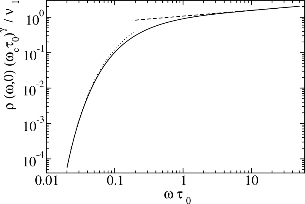
Figure 1: Zero-temperature crossover solution (III) for the TDoS (full curve) at $K=0.3$ and $N=5$. Here $\omega_{c}\tau_{0}=5\times 10^{4}$ was chosen, which is large enough to render results insensitive to its value. Dotted and dashed curves give the limiting expressions (46) and (45), respectively. Note the double-logarithmic scales.

Next we turn to the regime $T\tau_{0}\ll 1$ and $\omega\tau_{0}\ll 1$. The crossover function describing the transition from $\omega<T$ to $\omega>T$, reported in Ref. mishchenko , can be reproduced from Eq. (III) using asympotic expansions of $F_{1,2}$ and $H_{1,2}$. In particular, for $\omega\ll T\ll 1/\tau_{0}$,

$$\frac{\rho(T)}{\nu_{1}}=\frac{e^{{\rm C}\gamma+\gamma_{b}}}{(2\omega_{c}\tau_{0})^{\gamma}}\sqrt{\frac{\pi}{2.389}}\left(\frac{T\tau_{0}}{2\pi\gamma_{b}^{2}}\right)^{1/4}\,e^{-1.075\gamma_{b}\sqrt{2\pi/T\tau_{0}}}.$$ (47)

Finally, once either $T\tau_{0}\gg 1$ or $\omega\tau_{0}\gg 1$, typical values for $t$ in Eq. (III) are $t\sim{\rm min}(1/T,1/\omega)$, such that effectively the standard LL power laws are recovered. For $T\gg(1/\tau_{0},\omega)$,

$$\frac{\rho(T)}{\nu_{1}}\simeq\left(\frac{\pi}{2}\right)^{\gamma}\frac{\Gamma(1+\gamma)}{\Gamma^{2}(1+\gamma/2)}(T/\omega_{c})^{\gamma}.$$ (48)

IV Conductivity

IV.1 Interaction correction

In this section, we discuss the interaction correction to the Drude conductivity for arbitrary disorder, connecting the diffusive Altshuler-Aronov result aa with the ballistic limit, where Luttinger liquid power laws emerge. It is worth reiterating that weak localization corrections are not included in our theory, see Sec. II.2.

The Kubo formula determines the linear dc conductivity as the $q\to 0,i\omega_{m}\to\omega+i0^{+}$ limit of

$$\sigma(q,\omega_{m})=-\frac{e^{2}}{\omega_{m}}\langle j(q,\omega_{m})j(-q,-\omega_{m})\rangle+\frac{e^{2}\rho_{0}}{m\omega_{m}},$$ (49)

where $\rho_{0}$ is the Drude resistivity, $m$ the effective mass, and $j$ the particle current. The conductivity can alternatively be expressed as

$$\sigma(q,\omega_{m})=-(e/q)^{2}\,\omega_{m}\,P(q,\omega_{m}),$$ (50)

where the density-density correlator can be written as

$$P(q,\omega)=\frac{\langle\varphi(q,\omega)\varphi(-q,-\omega)\rangle}{U^{2}}-\frac{1}{U}.$$ (51)

Starting from the full action in the original formulation, see Eq. (II.2), the formula (51) may be derived as follows: Introduce a source field $\eta(q,\omega_{m})$ that is added to $\varphi$ in the tracelog only. The density correlator then follows from the resulting generating functional $Z[\eta]$ by means of

$$P(q,\omega_{m})=\left(\frac{\partial^{2}\ln Z}{\partial\eta(q,\omega_{m})\partial\eta(-q,-\omega_{m})}\right)_{\eta=0}.$$ (52)

Under the local gauge transformation (15), $\eta$ remains invariant, and one can safely perform the shift $\varphi\to\varphi-\eta$ in the action. After that shift, it is a simple matter to carry out the derivatives in Eq. (52) and to arrive at Eq. (51). In what follows, we use the intermediate cutoff $\omega_{c}^{\prime}$ and the mean free time $\tau^{\prime}_{0}=\tau_{0}(\omega_{c}^{\prime}/\omega_{c})^{\gamma_{i}}$ with the exponent (37), see Sec. II.5. After the corresponding RG procedure, the remaining interactions are treated by a first-order perturbation theory approach.

The classical Drude conductivity can now be recovered by our formalism as follows. Dropping all $B$ fluctuations in Eq. (II.5), the action up to quadratic order in $\varphi$ is $S_{\varphi}$, given by Eqs. (41) and (42). Keeping only $S_{\varphi}$, we may then apply Eq. (50), continue to real frequencies and arrive at the Drude conductivity

$$\sigma^{\prime}_{D}=e^{2}\nu_{1}v^{2}_{F}\tau^{\prime}_{0}=\frac{Ne^{2}v_{F}}{\pi\hbar}\tau^{\prime}_{0}.$$ (53)

This result includes an interaction correction encoded in the high-frequency RG scheme above. When substituting $\tau^{\prime}_{0}\to\tau_{0}$, one recovers the standard (noninteracting) Drude conductivity,

$$\sigma_{D}=e^{2}\nu_{1}v_{F}^{2}\tau_{0}.$$

We mention in passing that the above approximation also obtains the correct ac Drude form of the optical conductivity

$$\sigma_{D}(\omega)=\sigma_{D}/(1-i\omega\tau_{0}).$$ (54)

Interaction corrections to the dc Drude conductivity (53), defined via $\sigma=\sigma^{\prime}_{D}+\delta\sigma^{\prime}$, are obtained by inclusion of (i) $B$ fluctuations, and (ii) higher-order contributions in $\varphi$ to the action. To lowest order in the interactions, these additional ingredients to the theory conspire to obtain the result

$$\frac{\sigma(T)}{\sigma_{D}} = (\omega_{c}\tau_{0})^{-\gamma_{i}/(1+\gamma_{i})}\Biggl{[}1+\gamma_{i}\ln(2\pi e^{-1-{\rm C}}T\tau_{0}^{\prime})$$ (55)

$$- \gamma_{i}{\rm Re}\int_{0}^{\infty}d\Omega\frac{F(\Omega)}{\Omega}\Biggl{(}\sqrt{\frac{\Omega}{\Omega+i/\tau^{\prime}_{0}}}-1$$

$$+ \frac{i}{2\tau^{\prime}_{0}(1+K)\sqrt{\Omega^{2}+i\Omega/\tau^{\prime}_{0}}}\Biggr{)}\Biggr{]},$$

with the function

$$F(\Omega)=\frac{\partial\left(\Omega{\rm coth}(\Omega/2T)\right)}{\partial\Omega}.$$ (56)

For weak interactions, it is justified to use the renormalized mean free time in the form

$$\tau_{0}^{\prime}=\tau_{0}(\omega_{c}\tau_{0})^{-\gamma_{i}/(\gamma_{i}+1)}.$$ (57)

Before turning to the derivation of this result, let us discuss its physical meaning. We first note that, up to the prefactor $(\omega_{c}\tau_{0})^{-\gamma_{i}/(\gamma_{i}+1)}$, the conductivity is a universal function of the interaction parameter $K$, the channel number $N$, and the parameter $T\tau_{0}^{\prime}$. Importantly, the crossover temperature separating the LL and the Altshuler-Aronov regions, respectively, is determined by the renormalized scale $\tau_{0}^{\prime}$. For $T\tau_{0}^{\prime}>1$ and $\gamma\ll 1$ Eq. (55) simplifies to

$${\sigma(T)\over\sigma_{D}}\simeq(\omega_{c}\tau_{0}^{\prime})^{-\gamma_{i}}\left[1+\gamma_{i}\ln(2\pi e^{-(1+C)}T\tau_{0}^{\prime})\right],\;\;T\gtrsim\tau^{\prime-1}.$$ (58)

Exponentiation of the logarithm obtains the familiar Luttinger liquid high-temperature power law mattis ; giamarchi ; gornyi ,

$$\frac{\sigma(T)}{\sigma_{D}}\simeq e^{-\gamma_{i}(1+{\rm C})}(2\pi T/\omega_{c})^{\gamma_{i}},\;\;T\gg\tau^{\prime-1},$$ (59)

otherwise obtained by stopping the RG procedure of Sec. II.5 at $T\gg\tau^{\prime-1}$. Governed by the single-impurity backscattering exponent $\gamma_{i}$ (cf. Eq. (37) and Ref. kane ), the exponentiated form is valid only at asymptotically large temperatures where multiple interference is negligible. In the complementary regime $T\tau_{0}^{\prime}\ll 1$ the interaction correction becomes

$$\frac{\sigma-\sigma_{D}}{\sigma_{D}}\simeq-\gamma_{i}\frac{3\sqrt{\pi/2}\ \zeta(-1/2)}{1+K}(T\tau^{\prime}_{0})^{-1/2},$$ (60)

where $\zeta$ is the Riemann zeta function gradsteyn . This expression recovers the well-known $T^{-1/2}$ Altshuler-Aronov correction in 1D aa , leading to a pronounced suppression of the conductivity at low temperatures. At very low temperatures, this correction becomes sizeable and our first-order perturbative approach ceases to be valid. In that case, also quantum interference corrections have to be included.

The crossover solution (55) smoothly interpolates between the limits (59) and (60), respectively, as is shown for $K=0.9$ and $N=30$ in Figure 2. Note that Eqs. (59) and (60) match each other at $T\tau_{0}^{\prime}$ of order unity. Related crossover scenarios from diffusive dynamics at low temperatures to non-diffusive dynamics at high temperature have been discussed in earlier work. Specifically, in Refs. zaikin1 ; zaikin2 , the conductance of a quantum dot array was considered. In that system the high-temperature regime is governed by the chaotic dynamics of individual quantum dots. The latter differs strikingly from the ballistic dynamics of clean quantum wires which is why the results obtained for the high-temperature conductivity corrections are quantitatively different from ours. (Nonetheless, the qualitative high-$T$ profile looks similar, cf. Fig. 2 of Ref. zaikin1 .)

We finally note that our calculation above ignores finite-size effects, which are of minor importance in sufficiently long wires with good contact to external leads, where the resistance is dominated by the intrinsic part. Note also that four-terminal resistance measurements allow to circumvent boundary effects as long as the electrodes act as non-invasive probes. In both cases, the conductivity is the relevant transport coefficient. This regime has been experimentally studied in carbon nanotubes and other quantum wires for many years by now. In particular, linear voltage drops along a MWNT can be measured and have been reported in Ref. afm .

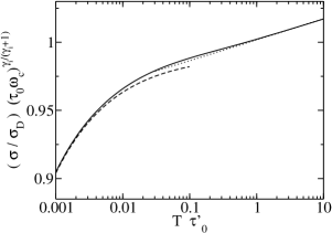
Figure 2: Temperature dependence of the conductivity (55) for $K=0.9$ and $N=30$. The limiting behaviors (59) and (60) are shown as dotted and dashed curves, respectively.

IV.2 Derivation

Let us now sketch the derivation of Eq. (55). For notational simplicity, the primes in $\tau^{\prime}_{0}$ and $\omega_{c}^{\prime}$ will be omitted for the moment. Our strategy is as follows: We expand Eq. (II.5) to second order in $B$-fluctuations, and integrate them out. This will generate an effective action for $\varphi$, which we expand up to fourth order. In addition, for internal consistency, the $B$-independent terms in Eq. (II.5) must also be kept up to fourth order. Schematically, our starting action then reads

$$S=S_{\varphi}+S_{B}+S_{4}^{(1)}+S_{4}^{(2)}.$$ (61)

The interaction correction results from the last three terms. The contribution $S_{B}$ combines (i) terms of second order in $B_{0,1}$ but zeroth order in $\varphi$, and (ii) of first order in $B$ but second order in $\varphi$. Note that the first order in both $B$ and $\varphi$ is strictly zero, due to our choice of the saddle point. Moreover, contributions to second order in $B$ and first or second order in $\varphi$ identically vanish in the replica limit. Finally,

$$S_{4}^{(1)}=\frac{\pi\nu_{1}v_{F}}{4}\sum_{C}{\rm Tr}(G_{C}\Gamma_{C})^{4}$$ (62)

comes from $B$-independent terms in the expansion of the tracelog in Eq. (II.5), while

$$S_{4}^{(2)}=\frac{\pi\nu_{1}}{8\tau_{0}}\left(\frac{1}{12}{\rm Tr}K_{2}^{4}-\frac{1}{3}{\rm Tr}\Lambda K_{2}\Lambda K_{2}^{3}+\frac{1}{4}{\rm Tr}\Lambda K_{2}^{2}\Lambda K_{2}^{2}\right)$$ (63)

similarly follows from the second term in Eq. (II.5).

Since Eq. (51) involves only $\varphi$, the $B$-fluctuations can be integrated out at the level of the action, replacing $S_{B}$ effectively by a new fourth-order term $S_{4}^{(3)}[\varphi]$. The lengthy but straightforward derivation of this term is detailed in Appendix C. Defining $S_{4}\equiv S_{4}^{(1)}+S_{4}^{(2)}+S_{4}^{(3)}$, the lowest-order correction to the conductivity, Eq. (51), is obtained by first-order expansion in $S_{4}$,

$$\delta P(q,\omega)=-U^{-2}\left\langle\varphi(q,\omega)\varphi(-q,-\omega)[S_{4}-\langle S_{4}\rangle_{S_{\varphi}}]\right\rangle_{S_{\varphi}}.$$ (64)

Loosely speaking, fluctuations of the $\varphi$ field ($S^{(1)}_{4},S^{(2)}_{4}$) describe the RPA screening of the Coulomb interaction by impurity-dressed Green functions (’empty bubble’), while joint fluctuations of the $B$ and the $\varphi$ field ($S^{(3)}_{4}$) account for the vertex renormalization of the RPA bubbles by impurity ladders. Accordingly, we will find that $S^{(3)}_{4}$ holds responsible for the corrections to the conductivity showing the strongest low-temperature singularities. Conversely, the terms $S^{(1)}_{4},S^{(2)}_{4}$ dominantly contribute to the conductivity in the Luttinger limit $T\tau_{0}^{\prime}>1$.

Doing the $\varphi$-contractions, we obtain for the conductivity

$$\delta\sigma = -\sigma_{D}\,{\rm Im}\int\frac{d\Omega}{\pi}F(\Omega)\int\frac{dq}{2\pi}\Pi_{0,R}^{-1}(q,\Omega)$$

$$\times (v_{F}q)^{2}{(K_{1}+K_{2}+K_{3})(q,\Omega)\over(v_{F}^{2}q^{2}-\Omega^{2}-i\Omega/\tau_{0})^{2}},$$

with the auxiliary quantities

$$K_{1}(q,\Omega) = 4\Bigl{(}1+\frac{1-2i\Omega\tau_{0}}{(2v_{F}q\tau_{0})^{2}+(1-2i\Omega_{0}\tau_{0})^{2})}\Bigr{)},$$

$$K_{2}(q,\Omega) = -2,$$

$$K_{3}(q,\Omega) = \frac{1}{\tau_{0}^{2}(v_{F}^{2}q^{2}-\Omega^{2}-i\Omega/\tau_{0})}\times$$

$$\times \frac{2-6i\Omega\tau_{0}-(2\Omega\tau_{0})^{2}+(2v_{F}q\tau_{0})^{2}}{(1-2i\Omega\tau_{0})^{2}+(2v_{F}q\tau_{0})^{2}},$$

where the function $F(\Omega)$ has been defined in (56). The contributions $K_{1,2,3}$ stem from $S_{4}^{(1,2,3)}$, respectively, and $\Pi_{0,R}^{-1}$ denotes the retarded function corresponding to $\Pi_{0}^{-1}$, see Eq. (42). Specifically, the ’ballistic contributions’ $K_{1,2}$ result from summing 12 terms corresponding to the diagrams in Fig. 3, followed by analytic continuation to real frequencies. (Although standard in principle, the actual calculation obtaining these terms, in particular the analytic continuation to real frequencies for the product of four Green functions, is rather involved. We refer to Appendix A of Ref. zna for related technical details.) The calculation of the third term $K_{3}$ is detailed in Appendix C. Dominating in the diffusive limit, it obtains the standard 1D Altshuler-Aronov correction aa , see Eq. (60).

Figure 3: Diagrams corresponding to $S_{4}^{(1)}$ and $S_{4}^{(2)}$ in the conductivity calculation. The contraction of $S_{4}^{(1)}$ or $S_{4}^{(2)}$ with $\varphi(q,\omega)\varphi(-q,-\omega)$ (denoted by $\varphi(\pm)$, respectively) leads to the pairing of $\varphi(\pm)$ with two different $\Gamma_{C}$ (or $K_{2}$ in the case of $S_{4}^{(2)}$), implying $12$ different contractions. Due to the cyclic invariance of the trace, only three different contributions emerge, depending on the $\Gamma_{C}$ ordering. Solid curves represent schematically the trace, external dotted lines the two $\Gamma_{C}$ connected to $\varphi(\pm)$, and dashed-dotted lines the pairing between the remaining $\Gamma_{C}$.

Equation (IV.2) implies the total correction to the Drude conductivity to lowest order in the interaction,

$$\delta\sigma = -2\sigma_{D}U\,\,{\rm Im}\int\frac{d\Omega}{\pi}F(\Omega)\int\frac{dq}{2\pi}$$

$$\times \frac{v_{F}^{2}q^{2}\left[v_{F}^{2}q^{2}+(1/\tau_{0}-i\Omega)^{2}\right]}{(v_{F}^{2}q^{2}-\Omega^{2}-i\Omega/\tau_{0})^{2}(v^{2}q^{2}-\Omega^{2}-i\Omega/\tau_{0})},$$

where $v=v_{F}/K$, see Eq. (8). After carrying out the final momentum integration and restoring primed quantities, we arrive at the preliminary result

$$\delta\sigma^{\prime} = -\gamma_{i}\sigma^{\prime}_{D}{\rm Re}\int_{0}^{\omega_{c}^{\prime}}d\Omega\frac{F(\Omega)}{\Omega}\Biggl{[}\sqrt{\frac{\Omega}{\Omega+i/\tau^{\prime}_{0}}}$$

$$+ \frac{i}{2\tau^{\prime}_{0}(1+K)\sqrt{\Omega^{2}+i\Omega/\tau^{\prime}_{0}}}\Biggr{]},$$

which may give the misleading impression that the conductivity depends on the somewhat arbitrary cutoff $\omega_{c}^{\prime}$. Noting that $\omega_{c}^{\prime}\tau_{0}^{\prime}\gtrsim 1$, to first order in the interaction, we have

$$\tau^{\prime}_{0}=\frac{\tau_{0}}{(\omega_{c}\tau_{0})^{\gamma_{i}/(\gamma_{i}+1)}}\left(1+\gamma_{i}\ln(\tau^{\prime}_{0}\omega_{c}^{\prime})\right),$$

leading to the estimate (57). Splitting off the UV divergent part in Eq. (IV.2) leads to the logarithmic term in Eq. (55), while the upper limit can be sent to infinity for the remaining integral in Eq. (IV.2). We finally arrive at the $\omega_{c}^{\prime}$-independent form (55).

V Conclusion

In this paper, we have developed a low-energy field theory of weakly interacting disordered multi-channel conductors. The theory is formulated in terms of two auxiliary fields, a scalar field $\varphi(x,\tau)$ decoupling the electron-electron interactions, and a matrix field $Q_{C}(x,\tau,\tau^{\prime})$ decoupling the effective interactions arising from the disorder ensemble average. The two fields $\varphi$ and $Q_{C}$ are coupled by a gauge mechanism. For general values of interaction/disorder/channel number, the theory is governed by a nonlinear action — the notorious ’tracelog’ — and remains difficult to evaluate. However, in a number of important cases analytical progress is possible. Specifically, at energies $\epsilon<\tau_{0}^{-1}$ smaller than the elastic scattering rate, and for large channel numbers, we recover the diffusive interacting $\sigma$ modelfinkelstein with all the known consequences. In the opposite limit $\epsilon\gg\tau_{0}^{-1}$, an (asymptotically exact) mapping onto the familiar action of the Luttinger liquid is possible. Finally, for weak interactions, a low-order expansion of the tracelog in $\varphi$ and in the generators of $Q$-fluctuations becomes permissible.

Focusing on the latter regime, we apply the formalism to study the crossover of the tunneling DoS (previously described in Ref. mishchenko ) and the conductivity from the ballistic to the diffusive regime. In the ballistic limit, we recover the standard Luttinger liquid power law behaviors in these quantities, while in the diffusive limit, we obtain a pseudogap in the low-energy part of the TDoS and the $T^{-1/2}$ Altshuler-Aronov interaction correction. Our main results are Eq. (III) for the tunneling density of states, and Eq. (55) for the temperature dependence of the conductivity. We believe that these results, covering the entire crossover from ballistic to diffusive, will be valuable in understanding experimental data on nanotubes or nanowires.

Let us conclude by noting some of the open problems in this area. The question of what happens to the conductivity at very low $T$ cannot be answered by our lowest-order calculation. Relatedly, in order to treat the small-$N$ limit, new conceptual advances will be necessary. (Progress along this line has been reported in Ref.gornyi .) Other interesting open questions not addressed here include the weak localization correction and the magnetoconductivity, the inclusion of the spin degree of freedom, and a microscopic calculation of the dephasing time in 1D. These topics may be addressed by future work.

Appendix A Derivation of the effective model Hamiltonian

In this appendix we review how the model Hamiltonian (1) may be distilled from more microscopic descriptions of a quasi-1D conductor. Generally, the simplifying assumptions below are expected to hold for energies $\epsilon\lesssim\epsilon_{\perp}$, where $\epsilon_{\perp}$ is the characteristic energy scale related to transversal (to the cross section of the wire) excitations in the system. For $l<L_{\perp}$, we have $\epsilon_{\perp}\sim v_{F}/L_{\perp}$, where $L_{\perp}$ is a typical transverse width of the wire. For $l>L_{\perp}$, on the other hand, $\epsilon_{\perp}\sim v_{F}l/L_{\perp}^{2}$. Resolving phenomena on larger energy scales is a doable task which, however, requires a more refined (and less universal) modeling. Throughout, the phrase ’low energy’ refers to the regime $\epsilon<\epsilon_{\perp}$.

In the absence of disorder and interactions, a quasi-1D conductor is characterized by $N$ open channels energetically below the Fermi energy. The number $N\approx S_{\perp}/\lambda_{F}^{2}$ is often tunable, e.g., via doping or backgate voltages, where $S_{\perp}=L_{\perp}^{2}$. We assume that (i) $N\gg 1$ is sufficiently large to justify the approximations employed later on, and (ii) the Fermi energy is located sufficiently far away from the bottom of the bands formed by longitudinal momentum components to justify introduction of well-defined chiral (right- or left-moving, $C=R/L=\pm$) electron branches for each channel; clearly, this becomes problematic if the Fermi energy is close to the bottom of a band. Moreover, we shall (iii) focus on the case of spinless (or spin-polarized) electrons. The generalization to the spinful case does not pose conceptual problems and is left to future work.

Denoting the 1D coordinate as $x$ (where we assume that no confinement along this axis is present) and the transverse degrees of freedom as ${\bf r}_{\perp}$, the electron operator $\Psi_{e}({\bf r})$, with ${\bf r}=(x,{\bf r}_{\perp})$, can be expanded into the $N$ transverse eigenfunctions as

$$\Psi_{e}({\bf r})=\sum_{n=1}^{N}\sum_{C=R/L}e^{iCk_{n}x}\phi_{n}({\bf r}_{\perp})\psi_{nC}(x),$$ (69)

where $\phi_{n}({\bf r}_{\perp})$ are the transverse eigenmodes normalized according to

$$\int d{\bf r}_{\perp}\phi^{\ast}_{n}({\bf r}_{\perp})\phi_{m}({\bf r}_{\perp})=\delta_{nm}.$$ (70)

To give an example, for MWNTs, the eigenmodes, arising from the wrapping of a 2D graphene sheet onto a cylinder, are egger

$$\phi_{n}(y)=L_{\perp}^{-1/2}\exp(2\pi iny/L_{\perp}),$$ (71)

where $L_{\perp}=2\pi R_{0}$ for outermost-shell radius $R_{0}$ of the MWNT. Here, the transverse coordinate is the angular variable $y$, with $0<y\leq L_{\perp}$. For given confinement, each band intersects the Fermi surface at $k=\pm k_{n}$ with its own Fermi momentum $k_{n}$, where the slope is given by the respective Fermi velocity $v_{n}$. At low energy scales, the kinetic part of the Hamiltonian then is

$$H_{0}=-i\sum_{C}C\int dx\Psi_{C}^{\dagger}(x)\hat{v}\partial_{x}\Psi_{C}(x),$$ (72)

with $\hat{v}={\rm diag}(v_{1},v_{2},\ldots,v_{N})$. The noninteracting DoS is thus given by $\nu_{1}=\sum_{n=1}^{N}1/(\pi v_{n})$. To simplify matters, we neglect differences in the channel-dependent velocity, $v_{n}\to\langle v_{n}\rangle_{n}\equiv v_{F}$, where $v_{F}$ denotes the average channel velocity. As may be checked, e.g., by an explicit calculation of the diffusive two-point correlation function of the system, this assumption is permissible at low energies. For equal Fermi velocities, the kinetic part of the Hamiltonian assumes the form of $H_{0}$ in Eq. (1).

Next let us turn to the repulsive Coulomb interactions among the electrons in the QW. Starting from an arbitrary microscopic interaction potential $U_{micr}({\bf r},{\bf r}^{\prime})$, which incorporates external screening effects due to the substrate or surrounding gates, one arrives at a rather complicated 1D interaction Hamiltonian. At low energies, it is however sufficient to consider a simple model interaction, which is assumed to be long-ranged (e.g., a $1/r$ potential) on length scales larger than $L_{\perp}$. In that case, the long-range tail of the interaction is expected to dominate all relevant 1D Coulomb interaction matrix elements, such as

$$U_{nm}(x-x^{\prime}) = \int d{\bf r}_{\perp}d{\bf r}_{\perp}^{\prime}U_{micr}(x-x^{\prime},{\bf r}_{\perp},{\bf r}_{\perp}^{\prime})$$

$$\times |\phi_{n}({\bf r}_{\perp})|^{2}|\phi_{m}({\bf r}_{\perp}^{\prime})|^{2}.$$

For $|x-x^{\prime}|\gg L_{\perp}$, the potential $U_{micr}$ is basically independent of the transverse coordinates ${\bf r}_{\perp}$ and ${\bf r}^{\prime}_{\perp}$, implying that the projected interaction does not depend on the channel indices, $U_{mn}\to U(x-x^{\prime})$. The expansion (69) then leads to an effective contribution to the Hamiltonian,

$$H_{I} = \frac{1}{2}\sum_{n,m=1}^{N}\sum_{C_{1},C_{2},C_{3},C_{4}}\int dxdx^{\prime}U(x-x^{\prime})$$

$$\times e^{-i(C_{1}-C_{4})k_{n}x}e^{-i(C_{2}-C_{3})k_{m}x^{\prime}}$$

$$\times \psi^{\dagger}_{nC_{1}}(x)\psi^{\dagger}_{mC_{2}}(x^{\prime})\psi_{mC_{3}}(x^{\prime})\psi_{nC_{4}}(x).$$

Following the standard reasoning leading to LL models gogolin ; voit , for a long-ranged potential, electron-electron (e-e) backscattering ($C_{1}=-C_{4},C_{2}=-C_{3}$) processes will be strongly suppressed. Moreover, e-e Umklapp scattering is important only close to commensurabilities and will not be discussed here. For a long-ranged interaction, the dominant interaction process then corresponds to e-e forward scattering, where $C_{1}=C_{4}$ and $C_{2}=C_{3}$ in Eq. (A). Such processes describe interactions coupling the 1D density fluctuations, $H_{I}=\frac{1}{2}\int dxdx^{\prime}\rho(x)U(x-x^{\prime})\rho(x^{\prime})$. It is then justified to express $H_{I}$ in terms of the $q=0$ Fourier component of $U(x-x^{\prime})$, denoted by $U$. (In the clean case, up to multiplicative logarithmic corrections in most observables, this procedure also describes the case of the unscreened $1/r$ interaction gogolin .) We are then left with the simple 1D forward-scattering interaction (6). We mention in passing that e-e backscattering can be (partially) included by allowing for different interaction strengths $g_{4}$ and $g_{2}$ in the $\rho_{C}\rho_{C}$ and $\rho_{C}\rho_{-C}$ couplings, respectively gogolin . With minor modifications, our approach can be adjusted to this situation.

Finally, quenched disorder is included by starting from a short-ranged (3D) Gaussian random potential $V({\bf r})$, with the disorder average defined by its only nonvanishing cumulant

$$\langle V({\bf r})V({\bf r}^{\prime})\rangle_{dis}=\frac{1}{2\pi\nu_{3}\tau_{0}}\delta({\bf r}-{\bf r}^{\prime}),$$ (74)

where $\nu_{3}=\nu_{1}/S_{\perp}$ is the 3D noninteracting DoS and we assume that disorder is weak, $k_{n}l\gg 1$ for all $k_{n}$. With Eq. (69), we then obtain FS and BS scattering as in Eqs. (3) and (4), respectively, where

$$\hat{V}_{C,nn^{\prime}} = e^{-iC(k_{n}-k_{n^{\prime}})x}\int d{\bf r}_{\perp}\phi_{n}^{*}({\bf r}_{\perp})\phi_{n^{\prime}}({\bf r}_{\perp})V({\bf r}),$$

$$\hat{W}_{nn^{\prime}} = e^{-i(k_{n}+k_{n^{\prime}})x}\int d{\bf r}_{\perp}\phi_{n}^{*}({\bf r}_{\perp})\phi_{n^{\prime}}({\bf r}_{\perp})V({\bf r})$$

can be taken as independent random variables whose statistical properties follow from Eq. (74). To simplify matters, we assume the specific torus-type confinement (71). Unless one is interested in details of transverse fluctuations or other high-energy features, the precise form of the confinement potential is not expected to change the essential physics. Statistical correlations of $W_{nm}(x)$ can then be described by the simple form (5).

Appendix B Noninteracting limit of the NL${\sigma}$M

Let us here discuss the diffusive properties at $|q|l\ll 1,|\omega_{m}|\tau_{0}\ll 1$ of the NL$\sigma$M (II.5) in the noninteracting limit. Using the parametrization (33), we have two different types of quantum fluctuations, $B_{0}$ and $B_{1}$, where the latter break chiral symmetry. The $B_{1}$ modes have a gap, but nevertheless are not to be discarded since they couple to the massless $B_{0}$ fluctuations. We show this now on the Gaussian level, starting from the noninteracting version of Eq. (II.5),

$$S = \frac{\pi\nu_{1}}{8\tau_{0}}{\rm Tr}(Q_{R}Q_{L})+\frac{\pi\nu_{1}}{4}\sum_{C}{\rm Tr}\Bigl{[}D(\partial_{x}Q_{C})^{2}$$ (75)

$$+2C\Lambda(T_{C}^{-1}\partial_{x}T_{C})-2\hat{\epsilon}Q_{C}\Bigr{]},$$

where we put $v_{F}=1$ in intermediate steps. In order to recover the conventional NL$\sigma$M, we define the chirally symmetric field $Q_{0}=T_{0}\Lambda T_{0}^{-1}$ with $T_{0}=\exp(-W_{0}/2)$, and integrate over the massive modes $B_{1}$. Expanding $S$ to second order in $B_{1}$ (but zeroth order in $B_{0}$), the first term in Eq. (75) produces

$$-\frac{\pi\nu_{1}}{4\tau_{0}}{\rm Tr}(W_{1}^{2})=\frac{\pi\nu_{1}}{2\tau_{0}}{\rm Tr}(B_{1}^{\dagger}B_{1}),$$

see Eq. (34), which determines the mass gap of the fluctuation mode $B_{1}$ referred to in Sec. II.2. The remaining parts of the action (75) are then expanded to linear order in $B_{1}$, where only the $T^{-1}_{C}\partial_{x}T_{C}$ term gives a contribution. Here one has to be careful because of the non-commuting nature of $B_{0,1}$, but within a first-order expansion, no difficulties arise under the parametrization (33). Terms that are quadratic in $B_{1}$ or involve spatial derivatives of $B_{1}$ are neglected since they vanish at low energy and/or long length scales. We finally arrive at

$$S = \frac{\pi\nu_{1}}{2}{\rm Tr}\Bigl{(}D(\partial_{x}Q_{0})^{2}-2\hat{\epsilon}Q_{0}-W_{1}^{2}/2\tau_{0}$$

$$- iW_{1}[T_{0}^{-1}\partial_{x}T_{0},\Lambda]_{-}\Bigr{)}.$$

Next $B_{1}$ is integrated out, and we finally obtain the 1D diffusive action for $Q_{0}$,

$$S=\frac{\pi\nu_{1}}{4}\left(D{\rm Tr}(\partial_{x}Q_{0})^{2}-4{\rm Tr}(\hat{\epsilon}Q_{0})\right).$$ (76)

On the Gaussian level, keeping replica indices implicit, this results in

$$S = \frac{\pi\nu_{1}T^{2}}{2}\sum_{\epsilon_{n}>0,\epsilon_{m}<0}\int\frac{dq}{2\pi}$$

$$\times \left[Dq^{2}+(\epsilon_{n}-\epsilon_{m})\right]|B_{0;nm}(q)|^{2},$$

implying the usual diffusion pole.

We finally remark that at energies $\epsilon\gtrsim\epsilon_{\perp}$, the diffusion properties (e.g. of MWNTs) become anisotropic. These ’medium energy effects’ may be resolved by employing the full disorder correlator of the $W_{nm}(x)$, and decoupling the impurity four-fermion action in terms of a channel-dependent $Q$-field. One thus obtains a more structured theory wherein details of anisotropic transport are resolved.

Appendix C Interaction correction

Here we provide the derivation of $S_{4}^{(3)}$ and of the corresponding interaction correction, see Sec. IV.2. The expansion of Eq. (II.5) in $B$ yields

$$S_{B} = \frac{\pi\nu_{1}}{8\tau_{0}}{\rm Tr}[W_{1}\Pi_{3}W_{1}+W_{0}\Pi_{1}W_{0}$$

$$-W_{0}\Pi_{2}W_{1}+2W_{0}P_{0}+2W_{1}P_{1}],$$

with kernels

$$\Pi_{1}(q,\omega) = \frac{v_{F}^{2}q^{2}+|\omega|\left(|\omega|+1/2\tau_{0}\right)}{v_{F}^{2}q^{2}+(|\omega|+1/2\tau_{0})^{2}},$$

$$\Pi_{2}(q,\omega) = \frac{qv_{F}{\rm sgn}(\omega)/\tau_{0}}{v_{F}^{2}q^{2}+(|\omega|+1/2\tau_{0})^{2}},$$

$$\Pi_{3}(q,\omega) = \frac{\left(|\omega|+1/\tau_{0}\right)\left(|\omega|+1/2\tau_{0}\right)+v_{F}^{2}q^{2}}{v_{F}^{2}q^{2}+(|\omega|+1/2\tau_{0})^{2}}.$$

Moreover,

$$P_{0}(q_{0},\epsilon_{n},\epsilon_{n}-\omega_{0})=\sum_{C,\omega_{m}}\int\frac{dq}{2\pi}\Bigl{(}\Gamma_{C}(q,\omega_{m})$$

$$\times \Gamma_{C}(q_{0}-q,\omega_{0}-\omega_{m})I_{C}(q,\omega_{m},q_{0},\omega_{0})$$

$$+ K_{2}(q,\omega_{m})K_{2}(q_{0}-q,\omega_{0}-\omega_{m}){\rm sgn}(\epsilon_{n}-\omega_{m})\Bigr{)},$$

and

$$P_{1}(q_{0},\epsilon_{n},\epsilon_{n}-\omega_{0})=\sum_{C,\omega_{m}}(-iC)\int\frac{dq}{2\pi}\Bigl{(}\Gamma_{C}(q,\omega_{m})$$

$$\times \Gamma_{C}(q_{0}-q,\omega_{0}-\omega_{m})I_{C}(q,\omega_{m},q_{0},\omega_{0})\Bigr{)},$$

with the kernel

$$I_{C}(q,\omega_{m},q_{0},\omega_{0})=iv_{F}\,\int\frac{dp}{2\pi}G_{C}(p,\epsilon)$$

$$\times G_{C}(p-q_{0},\epsilon-\omega_{0})G_{C}(p-q,\epsilon-\omega_{m}).$$

The Gaussian $B$-fluctuations are then integrated out. Calling the resulting action $S_{4}^{(3)}$, we find

$$S_{4}^{(3)}=-\frac{\pi\nu_{1}}{4\tau_{0}}\sum_{q_{0},q_{1},q_{2}}\sum_{\omega_{0}>0,\omega_{1},\omega_{2}}\sum_{0\leq\epsilon_{n}\leq\omega_{0}}$$

$$\Bigg{\{}\Bigg{[}\sum_{C}\Gamma_{C}(q_{1},\omega_{1})\Gamma_{C}(q_{0}-q_{1},\omega_{0}-\omega_{1})$$

$$\times I_{C}(q_{0},\omega_{0},q_{1},\omega_{1})\left(1-\frac{iC}{4}\frac{\Pi_{2}(q_{0},\omega_{0})}{\Pi_{3}(q_{0},\omega_{0})}\right)$$

$$+K_{2}(q_{1},\omega_{1})K_{2}(q_{0}-q_{1},\omega_{0}-\omega_{1}){\rm sgn}(\epsilon_{n}-\omega_{1})\Bigg{]}$$

$$\times\Bigg{[}\sum_{C^{\prime}}\Gamma_{C^{\prime}}(q_{2},\omega_{2})\Gamma_{C^{\prime}}(-q_{0}-q_{2},-\omega_{0}-\omega_{2})$$

$$\times I_{C^{\prime}}(q_{0},\omega_{0},q_{0}+q_{2},\omega_{0}+\omega_{2})\left(1-\frac{iC^{\prime}}{4}\frac{\Pi_{2}(q_{0},\omega_{0})}{\Pi_{3}(q_{0},\omega_{0})}\right)$$

$$+K_{2}(q_{2},\omega_{2})K_{2}(-q_{0}-q_{2},-\omega_{0}-\omega_{2}){\rm sgn}(\epsilon_{n}-\omega_{0}-\omega_{2})\Bigg{]}$$

$$\times\left(\Pi_{1}(q_{0},\omega_{0})-\Pi^{2}_{2}(q_{0},\omega_{0})/4\Pi_{3}(q_{0},\omega_{0})\right)^{-1}$$

$$+\Bigg{[}\sum_{C}(-iC)\Gamma_{C}(q_{1},\omega_{1})\Gamma_{C}(q_{0}-q_{1},\omega_{0}-\omega_{1})$$

$$\times I_{C}(q_{0},\omega_{0},q_{1},\omega_{1})\Bigg{]}\Bigg{[}\sum_{C^{\prime}}(-iC^{\prime})\Gamma_{C^{\prime}}(q_{2},\omega_{2})$$

$$\times\Gamma_{C^{\prime}}(q_{0}-q_{2},\omega_{0}-\omega_{2})$$

$$\times I_{C^{\prime}}(q_{0},\omega_{0},q_{0}+q_{2},\omega_{0}+\omega_{2})\Bigg{]}/\Pi_{3}(q_{0},\omega_{0})\Bigg{\}}.$$

Equation (64) is then used to compute the conductivity correction. The contraction of $\varphi(q,\omega)\varphi(-q,-\omega)$ with $S_{4}^{(3)}$ leads to eight terms, with four different terms appearing twice each. These four terms are in fact two by two equivalent via the symmetry $\omega\to-\omega$. In particular, the two contributions with $-\omega$ vanish after the summation over $\epsilon_{n}$ is performed. The two possible contractions are (i) $q_{1}=-q_{2}=q$, $\omega_{1}=-\omega_{2}=\omega$, and (ii) $q_{1}=q$, $\omega_{1}=\omega$, $q_{2}=q-q_{0}$, $\omega_{2}=\omega-\omega_{0}$. The external momentum $q$ is now taken to zero, and we also let $\omega\to 0$ under the constraint ${\rm Re}\,\omega>0$. The $\epsilon_{n}$-summation can be done easily and yields, after the frequency shift $\omega_{0}\to\omega_{0}+\omega_{m}$,

$$\delta\sigma_{3} = -\frac{8v_{F}^{2}e^{2}\nu_{1}\tau_{0}^{3}}{\omega_{m}}\sum_{\omega_{0}>0,q_{0}}\frac{\omega_{0}+\omega_{m}-|\omega_{0}-\omega_{m}|}{\Pi_{0}(q_{0},\omega_{0})}$$

$$\times \bigg{[}X_{1}^{2}(q_{0},\omega_{0})\left(\Pi_{1}(q_{0},\omega_{0})-\Pi^{2}_{2}(q_{0},\omega_{0})/4\Pi_{3}(q_{0},\omega_{0})\right)^{-1}$$

$$+ X_{2}^{2}(q_{0},\omega_{0})/\Pi_{3}(q_{0},\omega_{0})\bigg{]},$$

where $\omega_{m}\to 0$ has been anticipated and we have used the abbreviations

$$X_{1}(q_{0},\omega_{0})=\frac{1}{4\tau_{0}^{2}}\sum_{C}\frac{C\Gamma_{C}(q_{0},\omega_{0})}{2iv_{F}q_{0}\varphi(q_{0},\omega_{0})}$$

$$\times\left(1-\frac{iC}{4}\frac{\Pi_{2}(q_{0},\omega_{0})}{\Pi_{3}(q_{0},\omega_{0})}\right)I_{C}^{0}(q_{0},\omega_{0})+\frac{i}{2\tau_{0}}\frac{K_{2}(q_{0},\omega_{0})}{iv_{F}q_{0}\varphi(q_{0},\omega_{0})},$$

$$X_{2}(q_{0},\omega_{0})=\frac{1}{4\tau_{0}^{2}}\sum_{C}\frac{(-i)\Gamma_{C}(q_{0},\omega_{0})}{2iv_{F}q_{0}\varphi(q_{0},\omega_{0})}I_{C}^{0}(q_{0},\omega_{0}),$$

$$I_{C}^{0}(q_{0},\omega_{0})=2\tau_{0}\,\frac{1/\tau_{0}+\omega_{0}-iCv_{F}q_{0}}{(1/2\tau_{0}+\omega_{0}-iCv_{F}q_{0})^{2}}.$$

The summation over $\omega_{0}$ is then replaced by a contour integral, with a line cut for $\Omega=i\omega_{0}=i\omega$. Performing the analytic continuation $i\omega=\omega^{\prime}+i0^{+}$ with $\omega^{\prime}\to 0$, we finally obtain $K_{3}$ in Eq. (IV.2).

References

- (1) A.O. Gogolin, A.A. Nersesyan, and A.M. Tsvelik, Bosonization and Strongly Correlated Systems (Cambridge University Press, Cambridge, 1998).
- (2) J. Voit, Rep. Prog. Phys. 58, 977 (1995).
- (3) C.L. Kane and M.P.A. Fisher, Phys. Rev. B 46, 15233 (1992).
- (4) D.C. Mattis, Phys. Rev. Lett. 32, 714 (1974).
- (5) A. Luther and I. Peschel, Phys. Rev. Lett. 32, 992 (1974).
- (6) W. Apel and T.M. Rice, Phys. Rev. B 26, R7063 (1982).
- (7) S. Andergassen, T. Enss, V. Meden, W. Metzner, U. Schollwöck, and K. Schönhammer, Phys. Rev. B 70, 075102 (2004).
- (8) B.L. Altshuler and A.G. Aronov, in Electron-electron Interactions in Disordered Solids, edited by A.L. Efros and M. Pollak (Elsevier, Amsterdam, 1985).
- (9) A. Kamenev and A. Andreev, Phys. Rev. B 60, 2218 (1999).
- (10) Yu.V. Nazarov, Sov. Phys. JETP Lett. 49, 126 (1989); Sov. Phys. JETP 68, 561 (1989).
- (11) E.G. Mishchenko, A.V. Andreev, and L.I. Glazman, Phys. Rev. Lett. 87, 246801 (2001).
- (12) G. Grüner, Density Waves in Solids (Addison-Wesley, Reading, 1994).
- (13) T. Giamarchi and H.J. Schulz, Phys. Rev. B 37, 325 (1988).
- (14) A. Furusaki and N. Nagaosa, Phys. Rev. B 47, 4631 (1993).
- (15) M. Ogata and H. Fukuyama, Phys. Rev. Lett. 73, 468 (1994).
- (16) N.P. Sandler and D.L. Maslov, Phys. Rev. B 55, 13808 (1997).
- (17) S.V. Malinin, T. Nattermann, and B. Rosenow, Phys. Rev. B 70, 235120 (2004).
- (18) I.V. Gornyi, A.D. Mirlin, and D.G. Polyakov, Phys. Rev. Lett. 95, 046404 (2005); ibid. 95, 206603 (2005).
- (19) K.A. Matveev and L.I. Glazman, Phys. Rev. Lett. 70, 990 (1993).
- (20) Once interchain hopping becomes relevant, coherent electron transfer among the chains is important and eventually induces a crossover into a Fermi liquid state. Such effects are implicitly contained in the model studied below, since the ’open channels’ directly represent the eigenmodes of the noninteracting clean system.
- (21) A. Bachtold, M. de Jonge, K. Grove-Rasmussen, P.L. McEuen, M. Buitelaar, and C. Schönenberger, Phys. Rev. Lett. 87, 166801 (2001).
- (22) K. Liu, Ph. Avouris, R. Martel, and W.K. Hsu, Phys. Rev. B 63, 161404(R) (2001).
- (23) E. Graugnard, P.J. de Pablo, B. Walsh, A.W. Ghosh, S. Datta, and R. Reifenberger, Phys. Rev. B 64, 125407 (2001).
- (24) R. Tarkiainen, M. Ahlskog, J. Penttila, L. Roschier, P. Hakonen, M. Paalanen, and E. Sonin, Phys. Rev. B 64, 195412 (2001); R. Tarkiainen, M. Ahlskog, M. Paalanen, A. Zyuzin , P. Hakonen, ibid. 71, 125425 (2005).
- (25) N. Kang et al., Phys. Rev. B 66, 241403(R) (2002).
- (26) A. Kanda, K. Tsukagoshi, Y. Aoyagi, and Y. Ootuka, Phys. Rev. Lett. 92, 036801 (2004).
- (27) R. Egger and A.O. Gogolin, Phys. Rev. Lett. 87, 066401 (2001).
- (28) L. Bartosch and P. Kopietz, Eur. Phys. J. B 28, 29 (2002).
- (29) T. Lorenz et al., Nature 418, 614 (2002).
- (30) E. Slot, M.A. Holst, H.S.J. van der Zant, and S.V. Zaitsev-Zotov, Phys. Rev. Lett. 93, 176602 (2004).
- (31) A.N. Aleshin, H.J. Lee, Y.W. Park, and K. Akagi, Phys. Rev. Lett. 93, 196601 (2004).
- (32) F. Liu, M. Bao, K.L. Wang, C. Li, B. Lei, and C. Zhou, Appl. Phys. Lett. 86, 213101 (2005).
- (33) L. Venkataraman, Y.S. Hong, and P. Kim, Phys. Rev. Lett. 96, 076601 (2006).
- (34) K.A. Matveev, D. Yue, and L.I. Glazman, Phys. Rev. Lett. 71, 3351 (1993).
- (35) A.M. Rudin, I.L. Aleiner, and L.I. Glazman, Phys. Rev. B 55, 9322 (1997).
- (36) G. Zala, B.N. Narozhny, and I.L. Aleiner, Phys. Rev. B 64, 214204 (2001).
- (37) I.V. Gornyi and A.D. Mirlin, Phys. Rev. Lett. 90, 076801 (2003).
- (38) A.M. Finkel’stein, Sov. Phys. JETP 57, 97 (1983).
- (39) D.S. Golubev and A.D. Zaikin, Phys. Rev. B 70, 165423 (2004).
- (40) D.S. Golubev, A.V. Galaktionov, and A.D. Zaikin, Phys. Rev. B 72, 205417 (2005).
- (41) The reason for avoiding bosonization is that a straightforward multi-channel generalization of the bosonized theory giamarchi does not properly describe the diffusive phase in the noninteracting limit. Technically, this failure can be traced to a breaking of the replica rotation symmetry originally present in the non-interacting model, yet absent in the (abelian) bosonized theory giamarchi . For related comments, see also Ref. gornyi .
- (42) For channel-dependent interactions beyond Eq. (6), and for non-uniformly distributed Fermi velocities additional terms may be generated. However, we do not believe these terms to be of physical relevance. Specifically, on the noninteracting level, and independently of fluctuations in the Fermi velocities, the correct (anisotropic) diffusion properties are recovered from impurity backscattering alone.
- (43) J. Zinn-Justin, Quantum Field Theory and Critical Phenomena, 4th edition (Oxford University Press, Oxford, 2002).
- (44) K. Fujikawa and H. Suzuki, Phys. Rep. 398, 221 (2004).
- (45) In the diagrammatic approach, the disordered Green function has a prefactor before , in contrast to Eq. (28). The difference arises here quite naturally.
- (46) There is an additional prefactor in Eq. (III), which we drop here. For and , it is very close to unity.
- (47) I.S. Gradshteyn and I.M. Ryzhik, Table of Integrals, Series, and Product (Academic Press, Inc., 1980).
- (48) The critical value follows by taking into account the disorder-induced renormalization of the interaction. This effect is only important for very low temperatures, a regime not considered in this paper.
- (49) T. Giamarchi, Quantum Physics in One Dimension (Oxford University Press, Oxford, 2004).
- (50) A. Bachtold, M.S. Fuhrer, S. Plyasunov, M. Forero, E.H. Anderson, A. Zettl, and P.L. McEuen, Phys. Rev. Lett. 84, 6082 (2000).