A variational approach to the moving contact line hydrodynamics

Abstract

In immiscible two-phase flows, contact line denotes the intersection of the fluid-fluid interface with the solid wall. When one fluid displaces the other, the contact line moves along the wall. A classical problem in continuum hydrodynamics is the incompatibility between the moving contact line and the no-slip boundary condition, as the latter leads to a non-integrable singularity. The recently discovered generalized Navier boundary condition (GNBC) offers an alternative to the no-slip boundary condition which can resolve the moving contact line conundrum. We present a variational derivation of the GNBC through the principle of minimum energy dissipation (entropy production), as formulated by Onsager for small perturbations away from the equilibrium. Through numerical implementation of a continuum hydrodynamic model, it is demonstrated that the GNBC can quantitatively reproduce the moving contact line slip velocity profiles obtained from molecular dynamics simulations. In particular, the transition from complete slip at the moving contact line to near-zero slip far away is shown to be governed by a power-law partial slip regime, extending to mesoscopic length scales. The sharp (fluid-fluid) interface limit of the hydrodynamic model, together with some general implications of slip versus no-slip, are discussed.

1 Introduction

The no-slip boundary condition states that there can be no relative motion at the fluid-solid interface (Batchelor 1991). It is generally regarded as a cornerstone in continuum hydrodynamics, owing to its proven applicability in diverse fluid-flow problems. However, decades ago it was discovered that in immiscible two-phase flows, the moving contact line (MCL), defined as the intersection of the fluid-fluid interface with the solid wall, is incompatible with the no-slip boundary condition (Moffatt 1964; Hua & Scriven 1971; Dussan & Davis 1974; Dussan 1976; Dussan 1979; de Gennes 1985). As shown by ?, under usual hydrodynamic assumptions, viz. incompressible Newtonian fluids, no-slip boundary condition, and smooth, rigid, solid walls, there is a velocity discontinuity at the MCL, and the tangential force exerted by the fluids on the solid bounding surface in the vicinity of the MCL is infinite. This is the well-known contact-line singularity. In the past two decades, it was shown through molecular dynamics (MD) simulations that near-complete slip indeed occurs at the MCL (Koplik, Banavar & Willemsen 1988; Koplik, Banavar & Willemsen 1989; Thompson & Robbins 1989; Thompson, Brinckerhoff & Robbins 1993). This finding presented a conundrum for classical hydrodynamics, due to a lack of viable alternatives apart from ad hoc fixes. Furthermore, in the absence of a viable boundary condition which can reproduce the MD results, accurate continuum description of immiscible flows in the micro- or nanoscales remained an elusive goal.

Through analysis of extensive MD data, it was recently discovered that there is indeed a differential boundary condition, denoted the generalized Navier boundary condition (GNBC), which resolves the MCL conundrum (Qian, Wang & Sheng 2003). Here we show that the GNBC can be derived variationally from the principle of minimum energy dissipation (Onsager 1931a and 1931b), and its implementation through the use of a Cahn-Hilliard (CH) free energy functional (Cahn & Hilliard 1958) leads to quantitative predictions in excellent agreement with MD simulation results. In what follows, the MCL problem is briefly recapitulated in Sec. 2. The variational derivation of the GNBC in Sec. 3 is followed by a numerical demonstration of its consequences in Sec. 4. It is shown that the transition from near-complete slip at the MCL to near-zero slip (no-slip) far away from the MCL is not confined to a molecular-sized region around the MCL. Instead, the transition follows a power-law profile of partial slipping, extending to mesoscopic scales (Qian, Wang & Sheng 2004). The sharp/diffuse (fluid-fluid) interface limits of our theory and their associated issues are described in Sec. 5. In Sec. 6 we discuss some general implications of replacing the no-slip boundary condition, which can be regarded as an approximation to the GNBC in single-phase flow regions, by the more accurate GNBC. In particular, it is argued that slip and partial slip boundary conditions offer the prospect of nanoscale interface engineering to “tune” the amount of slipping.

2 Recapitulation of the moving contact line problem

Consider an immiscible two-phase flow where one fluid displaces the other (see figure 1). If the no-slip boundary condition is applied along the wall, it can be shown that the tangential viscous stress varies as $\eta V/x$, where $\eta$ is the viscosity, $V$ is the wall speed in the reference frame where the fluid-fluid interface is stationary, and $x$ is the distance along the wall away from the MCL. This variation leads to diverging stress as $x\to 0$. In particular, this stress divergence is non-integrable and implies infinite (viscous) dissipation (Dussan & Davis 1974). Over the years there have been numerous models and proposals aiming to resolve this problem. For example, there have been the kinetic adsorption/desorption model by ?, the slip models by ?, ?, and ?, and the diffuse-interface models by ?, ?, ?, ?, and ?.

Figure 1: When one fluid displaces another immiscible fluid, the contact line is moving relative to the solid wall. Due to the contact-line motion, the dynamic contact angle $\theta_{d}$ deviates from the static contact angle $\theta_{s}$ which is determined by the Young equation $\gamma\cos\theta_{s}+\gamma_{2}=\gamma_{1}$.

In another approach to the MCL problem, ? carried out an asymptotic analysis and found, to the leading order in the capillary number $Ca=\eta V/\gamma$, a relation for the dependence of the apparent contact angle (the angle of the fluid-fluid interface at some mesoscopic distance away from the fluid-solid interface) on the microscopic contact angle, the capillary number, and the distance from the contact line over which slip occurs. In this approach, the details of the slip flow in the inner region around the MCL are absorbed into a model-dependent constant in the asymptotic relation. In particular, it has been shown that the asymptotic behavior is independent of the microscopic boundary condition(s) (Dussan 1976). But this conclusion only deepens the mystery of what happens at the contact line.

In the past two decades, MD simulations have shown that near-complete slip indeed occurs at the MCL (Koplik, Banavar & Willemsen 1988; Koplik, Banavar & Willemsen 1989; Thompson & Robbins 1989; Thompson, Brinckerhoff & Robbins 1993). Small amount of partial slipping was also observed in single-phase flows (Thompson & Robbins 1990; Thompson & Troian 1997; Barrat & Bocquet 1999a; Cieplak, Koplik & Banavar 2001). Such partial slip can be accounted for by the Navier boundary condition (NBC), proposed nearly two centuries ago by ?: $v^{slip}=l_{s}\dot{\gamma}$, where $v^{slip}$ is the slip velocity at the surface, measured relative to the (moving) wall, $l_{s}$ is the slip length, and $\dot{\gamma}$ is the shear rate at the surface. The small value of $l_{s}$ explains why the NBC is practically indistinguishable from the no-slip boundary condition in single-phase macroscopic flows.

While the NBC can account for the small amount of slip in high shear-rate single-phase flows, it fails to account, by an order of magnitude, for the near-complete slip at the MCL (Thompson & Robbins 1989; Thompson, Brinckerhoff & Robbins 1993). Recently, the MD-continuum hybrid simulation has been applied as a tool to investigate this problem by ?, and by ?. But such approaches leave unresolved the problem of MCL boundary condition. Lack of a viable boundary condition implies that accurate MCL description (and hence immiscible two-phase flows) can only be attained through MD simulations, in systems far too small compared with most of the experimentally achievable samples.

The recent discovery of the GNBC (Qian, Wang & Sheng 2003) resolves the MCL conundrum. The GNBC states that the slip velocity is proportional to the total tangential stress — the sum of the viscous stress and the uncompensated Young stress; the latter arises from the deviation of the fluid-fluid interface from its static configuration. Here we show the GNBC to be derivable from the principle of minimum energy dissipation. Its form is hence uniquely necessitated by the thermodynamics of immiscible two-phase flows.

3 Variational derivation of the moving contact line hydrodynamics

There is a minimum dissipation theorem for incompressible single-phase flows. According to ? (attributable to Helmholtz), “the rate of dissipation in the flow in a given region with negligible inertia forces is less than that in any other solenoidal velocity distribution (of zero divergence) in the same region with the same values of the velocity at all points of the boundary of the region.” The variational principles involving dissipation have been further developed in the works of ?, ?, ?, ?, and ?. In mathematical terms, if we ignore inertia forces for the moment (this can be added in at the end, see equation (3.36)) and let the variables $\alpha_{1},\cdot\cdot\cdot,\alpha_{n}$ describe the displacement from thermodynamic equilibrium, $\dot{\alpha_{1}},\cdot\cdot\cdot,\dot{\alpha_{n}}$ being the corresponding rates and $F(\alpha_{1},\cdot\cdot\cdot,\alpha_{n})$ the free energy, then for a set of simultaneous irreversible processes governed by

$$\sum_{j=1}^{n}\rho_{ij}\dot{\alpha}_{j}=-\displaystyle\frac{\partial F(\alpha_{1},\cdot\cdot\cdot,\alpha_{n})}{\partial\alpha_{i}},\;\;\;(i=1,\cdot\cdot\cdot,n),$$ (3.1)

where the coefficients $\rho_{ij}$ are introduced through the linear relations between the rates $\{\dot{\alpha_{i}}\}$ and the “forces” $\{-\partial F/\partial\alpha_{i}\}$, a variational principle (Onsager 1931a and 1931b) can be formulated, namely

$$\delta\left[\Phi(\dot{\alpha},\dot{\alpha})+\dot{F}(\alpha,\dot{\alpha})\right]=\sum_{i=1}^{n}\left(\displaystyle\frac{\partial\Phi}{\partial\dot{\alpha}_{i}}+\displaystyle\frac{\partial F}{\partial\alpha_{i}}\right)\delta\dot{\alpha}_{i}=0,$$ (3.2)

where $\Phi(\dot{\alpha},\dot{\alpha})$ is the dissipation-function defined by

$$\Phi(\dot{\alpha},\dot{\alpha})\equiv\displaystyle\frac{1}{2}\sum_{i,j}\rho_{ij}\dot{\alpha}_{i}\dot{\alpha}_{j},$$ (3.3)

and $\dot{F}(\alpha,\dot{\alpha})$ is the rate of change of the free energy:

$$\dot{F}(\alpha,\dot{\alpha})\equiv\sum_{i=1}^{n}\displaystyle\frac{\partial F(\alpha_{1},\cdot\cdot\cdot,\alpha_{n})}{\partial\alpha_{i}}\dot{\alpha}_{i}.$$ (3.4)

Microscopic reversibility requires the reciprocal relations $\rho_{ij}=\rho_{ji}$. We note that the variation in equation (3.2) should be taken with respect to the rates $\{\dot{\alpha_{i}}\}$ for prescribed $\{\alpha_{i}\}$, and the extremum given by equation (3.2) is always a minimum because $\Phi(\dot{\alpha},\dot{\alpha})$ is quadratic in $\{\dot{\alpha_{i}}\}$ and positive definite (Onsager 1931b). The dissipation-function $\Phi$ as given by equation (3.3) is noted to be half the rate of energy dissipation, owing to the required consistency between the “force balance” condition (3.1), the minimum condition (3.2), and the fact that the dissipative forces are linear in rates. It can be shown that the principle of minimum energy dissipation yields the most probable course of an irreversible process, provided the displacements from thermodynamic equilibrium are small (Onsager 1931b, Onsager & Machlup 1953). We note that the variational principle presented here is a special form of the principle of minimum energy dissipation formulated by Onsager. First, the dissipation-function $\Phi$ defined here is different from that by Onsager by a factor of $T$, the temperature which is assumed to be uniform in the fluids. Second, the rate of change of the free energy $\dot{F}$ equals $-T\dot{S}+\dot{W}$, where $S$ and $W$ denote the entropy and work, respectively (Doi 1983). This point will be elaborated after equation (3.24). In Appendix A we use a single-variable case to illustrate the underlying physics of the principle of minimum energy dissipation.

When applied to a single-phase flow confined by solid surfaces, the variational principle in equation (3.2) becomes

$$\delta\Phi(\dot{\alpha},\dot{\alpha})=\sum_{i=1}^{n}\displaystyle\frac{\partial\Phi}{\partial\dot{\alpha}_{i}}\delta\dot{\alpha}_{i}=0.$$ (3.5)

Here the rates $\{\dot{\alpha_{i}}\}$ correspond to the velocity field ${\bf v}({\bf r})$ and the $\dot{F}(\alpha,\dot{\alpha})$ term defined by equation (3.4) drops out in the variation because there is no such free energy $F(\{\alpha_{i}\})$ in single-phase flows. As the dissipation-function $\Phi(\dot{\alpha},\dot{\alpha})$ equals half the rate of energy dissipation, equation (3.5) leads directly to the minimum dissipation theorem by Helmholtz (Batchelor 1991). That is, once the values of the velocity are prescribed at the solid surfaces, the rate of viscous dissipation is minimized by the solution of the Stokes equation. Physically, when fluid slipping occurs at the solid surface, there is dissipation at the fluid-solid interface as well. Below we show that to minimize the total rate of energy dissipation $R_{1}\left[{\bf v}\right]$ $(=2\Phi(\dot{\alpha},\dot{\alpha}))$, the incompressible flow has to satisfy the Stokes equation and the NBC simultaneously. Mathematically, this means that the Stokes equation

$$-\nabla p+\eta\nabla^{2}{\bf v}=0,$$ (3.6)

and the NBC

$$\beta v_{\tau}^{slip}=-\sigma^{visc}_{n\tau}=-\eta(\partial_{n}v_{\tau}+\partial_{\tau}v_{n}),$$ (3.7)

can be derived by minimizing the functional

$$R_{1}\left[{\bf v}\right]=\int d{\bf r}\left[\displaystyle\frac{\eta}{2}(\partial_{i}v_{j}+\partial_{j}v_{i})^{2}\right]+\int dS\left[\beta\left(v_{\tau}^{slip}\right)^{2}\right],$$ (3.8)

with respect to the velocity distribution. Here $p$ is the pressure which plays the role of the Lagrange multiplier for the incompressibility condition $\nabla\cdot{\bf v}=0$, $\eta$ is the shear viscosity, $\beta$ is the slip coefficient, subscript $n$ denotes the outward surface normal, subscript $\tau$ denotes the direction tangential to the surface, $v_{\tau}^{slip}$ is the slip velocity, defined as the tangential fluid velocity at the solid surface, measured relative to the (moving) wall, $\sigma^{visc}_{n\tau}$ is the $n\tau$ component of the Newtonian viscous stress tensor, and $\int dS$ denotes the integration over the solid surface. The functional $R_{1}[{\bf v}]$ is $2\Phi(\dot{\alpha},\dot{\alpha})$ for single-phase flows, measuring the total rate of dissipation due to viscosity in the bulk and slipping at the solid surface. We write the single-phase flow dissipation $R_{1}$ as the sum of $R_{v}$ due to viscosity and $R_{s}$ due to slipping: $R_{1}=R_{v}+R_{s}$, with

$$R_{v}\left[{\bf v}\right]=\int d{\bf r}\left[\displaystyle\frac{\eta}{2}(\partial_{i}v_{j}+\partial_{j}v_{i})^{2}\right]$$ (3.9)

and

$$R_{s}\left[{\bf v}\right]=\int dS\left[\beta\left(v_{\tau}^{slip}\right)^{2}\right].$$ (3.10)

While $R_{s}$ may appear to be very different from $R_{v}$ in form, yet in reality the two terms are very similar if it is realized that $v_{\tau}^{slip}$ is just the tangential velocity difference/differential at the fluid-solid interface. Hence $\beta$ is just the viscosity divided by a length scale $l_{s}$, defined as the slip length. Associated with the variation of the velocity field ${\bf v}({\bf r})\to{\bf v}({\bf r})+\delta{\bf v}({\bf r})$, the change in $R_{v}$ is given by

$$\delta R_{v}=-2\eta\int d{\bf r}\left[\partial_{j}\left(\partial_{j}v_{i}+\partial_{i}v_{j}\right)\delta v_{i}\right]+2\eta\int dS\left[\partial_{n}v_{\tau}\delta v_{\tau}+\partial_{\tau}v_{n}\delta v_{\tau}\right],$$ (3.11)

and that in $R_{s}$ given by

$$\delta R_{s}=2\beta\int dS\left[v_{\tau}^{slip}\delta v_{\tau}\right].$$ (3.12)

Imposing the incompressibility condition $\partial_{i}v_{i}=0$ by the use of a Lagrange multiplier $\alpha({\bf r})$ leads to one more term $\int d{\bf r}\left[\alpha\partial_{i}v_{i}\right]$, whose variation is given by

$$\delta\int d{\bf r}\left[\alpha\partial_{i}v_{i}\right]=-\int d{\bf r}\left[\partial_{i}\alpha\delta v_{i}\right].$$ (3.13)

Here the boundary condition $v_{n}=0$ has been used at the solid surface, where only $\delta v_{\tau}$ is allowed. From equations (3.11), (3.12), and (3.13), we obtain the Euler-Lagrange equations

$$-2\eta\partial_{j}\left(\partial_{j}v_{i}+\partial_{i}v_{j}\right)-\partial_{i}\alpha=0$$ (3.14)

in the bulk and

$$2\eta\left(\partial_{n}v_{\tau}+\partial_{\tau}v_{n}\right)+2\beta v_{\tau}^{slip}=0$$ (3.15)

at the surface. Note that equation (3.14) is identical to the Stokes equation (3.6) with $\partial_{j}v_{j}=0$ and $\alpha=-2p$, and equation (3.15) reduces to the NBC (3.7). That equations (3.6) and (3.7) can both be derived variationally from the minimization of $R_{1}$ is a generalization of the minimum dissipation theorem by taking into account fluid slipping at the solid surface.

It should be emphasized that while $R_{s}$ arises from the assumption of fluid-solid interface slipping, there is no specification of how much slipping there should be. In other words, even an infinitesimal amount of interface slipping would lead to equations (3.6) and (3.7). In particular, the no-slip boundary condition is obtained in the limit of $\beta\to\infty$, corresponding to a vanishing slip length $l_{s}=\eta/\beta$. In the other limit, $\beta\to 0$, we would have only the first term on the right-hand side of equation (3.8), and $\sigma^{visc}_{n\tau}=0$ on the boundary. Thus the NBC interpolates between the zero tangential viscous stress limit and the no-slip limit.

To generalize the functional $\Phi(\dot{\alpha},\dot{\alpha})=\frac{1}{2}R_{1}[{\bf v}]$ from single-phase to immiscible two-phase flows, it is recognized that a free energy functional is required to stabilize the interface separating the two immiscible fluids. Hence the introduction of a Landau free energy functional ${\cal F}[\phi({\bf r})]$ is a necessity, presumably of the form (Cahn & Hilliard 1958; Bray 1994)

$${\cal F}[\phi({\bf r})]=\int d{\bf r}\left[\displaystyle\frac{K}{2}\left(\nabla\phi\right)^{2}+f(\phi)\right],$$ (3.16)

where the potential $f(\phi)$ has a double-well structure. Here the phase field $\phi({\bf r})$ measures the (conserved) composition locally defined by $\phi=(\rho_{2}-\rho_{1})/(\rho_{2}+\rho_{1})$, with $\rho_{1}$ and $\rho_{2}$ being the number densities of the two fluid species. We also introduce the interfacial free energy per unit area at the fluid-solid interface, $\gamma_{fs}(\phi)$, which is a function of the local composition. Two quantities $\mu$ and $L$ can be defined from the variation of the total free energy

$$F={\cal F}[\phi]+\int dS\left[\gamma_{fs}(\phi)\right],$$

that is,

$$\delta\left\{{\cal F}[\phi]+\int dS\left[\gamma_{fs}(\phi)\right]\right\}=\int d{\bf r}\left[\mu\delta\phi\right]+\int dS\left[L\delta\phi\right],$$ (3.17)

in which $\mu=\delta{\cal F}/\delta\phi=-K\nabla^{2}\phi+\partial f(\phi)/\partial\phi$ by definition is the chemical potential and $L$, given by $K\partial_{n}\phi+\partial\gamma_{fs}(\phi)/\partial\phi$, is the corresponding quantity at the solid surface. Minimizing the total free energy with respect to $\phi$ yields the equilibrium conditions $\mu=C$ in the bulk and $L=0$ at the surface, $C$ being a constant acting as the Lagrange multiplier for the conservation of $\phi$. It will be shown later that $L=0$ leads to the Young equation for the static contact angle.

From the equilibrium conditions derived above, we see that deviations from the two-phase equilibrium may be measured by the “forces” $\nabla\mu$ in the bulk and $L$ at the fluid-solid interface. For small perturbations away from the equilibrium, the additional rate of dissipation $R_{\phi}$ arises from system responses that are linear in $\nabla\mu$ and $L$. Such responses are described by the diffusive current $\bf J$ in the bulk and the material time derivative of $\phi$ at the solid surface, i.e., $\dot{\phi}=\partial\phi/\partial t+v_{\tau}\partial_{\tau}\phi$. The conservation of $\phi$ means that the diffusive current and the material time derivative of $\phi$ satisfy the continuity equation

$$\dot{\phi}\equiv\displaystyle\frac{\partial\phi}{\partial t}+{\bf v}\cdot\nabla\phi=-\nabla\cdot{\bf J}.$$ (3.18)

But at the fluid-solid interface, diffusive transport normal to the interface is possible ($\partial_{n}J_{n}\neq 0$ in general), hence the interfacial $\phi$ is not conserved. In anticipation of the relevant dynamics governing the conserved $\phi$ in the bulk and nonconserved interfacial $\phi$, $\bf J$ in the bulk and $\dot{\phi}$ at the solid surface are hence the two additional rates associated with the coexistence of two phases. The additional rate of dissipation $R_{\phi}$ due to the displacement from the two-phase equilibrium may be constructed as a functional quadratic in the rates, $R_{\phi}=R_{d}+R_{r}$, where

$$R_{d}=\int d{\bf r}\left[\displaystyle\frac{{\bf J}^{2}}{M}\right],$$ (3.19)

and

$$R_{r}=\int dS\left[\displaystyle\frac{\dot{\phi}^{2}}{\Gamma}\right],$$ (3.20)

with $M$ and $\Gamma$ introduced as two phenomenological parameters. Combining $R_{\phi}$ with $R_{1}$ in equation (3.8), we obtain the dissipation-function $\Phi(\dot{\alpha},\dot{\alpha})$ for immiscible two-phase flows:

$$\Phi=\int d{\bf r}\left[\displaystyle\frac{\eta}{4}(\partial_{i}v_{j}+\partial_{j}v_{i})^{2}\right]+\int dS\left[\displaystyle\frac{\beta}{2}\left(v_{\tau}^{slip}\right)^{2}\right]+\int d{\bf r}\left[\displaystyle\frac{{\bf J}^{2}}{2M}\right]+\int dS\left[\displaystyle\frac{\dot{\phi}^{2}}{2\Gamma}\right],$$ (3.21)

which equals half the total rate of energy dissipation $R_{2}$ in two-phase flows, i.e.,

$$\Phi=\displaystyle\frac{1}{2}R_{2}=\displaystyle\frac{1}{2}(R_{1}+R_{\phi})=\displaystyle\frac{1}{2}(R_{v}+R_{s}+R_{d}+R_{r}),$$ (3.22)

Now the viscosity $\eta$ and slip coefficient $\beta$ in equation (3.21), respectively, are understood to take on their respective values for the two immiscible fluids on two sides of the interface. Note that the right-hand side of equation (3.21) consists of four terms, contributed by the four physically distinct sources of dissipation — the shear viscosity in the bulk, the fluid slipping at the solid surface, the composition diffusion in the bulk, and the composition relaxation at the solid surface. In addition, each term that contributes to $\Phi$ is positive definite and quadratic in a rate that arises from the displacement from the equilibrium and accounts for a particular source of dissipation. This quadratic dependence follows the general rule governing entropy production in a thermodynamic process (Landau & Lifshitz 1997), it directly arises from the linear response to a small perturbation away from the equilibrium.

The rate of change of the free energy, i.e., $\dot{F}(\alpha,\dot{\alpha})$ in equation (3.4), may be written as

$$\dot{F}=\int d{\bf r}\left[\mu\displaystyle\frac{\partial\phi}{\partial t}\right]+\int dS\left[L\displaystyle\frac{\partial\phi}{\partial t}\right],$$ (3.23)

in accordance with the variation of the total free energy in equation (3.17). Substituting ${\partial\phi}/{\partial t}=\dot{\phi}-{\bf v}\cdot\nabla\phi$ into equation (3.23) and using $\int d{\bf r}\left[\mu\dot{\phi}\right]=\int d{\bf r}\left[-\mu\nabla\cdot{\bf J}\right]=\int d{\bf r}\left[\nabla\mu\cdot{\bf J}\right]$ with $\int d{\bf r}\left[\nabla\cdot(\mu{\bf J})\right]=\int dS\left[\mu J_{n}\right]=0$ because of the impermeability condition $J_{n}=0$ at the solid surface, we obtain

$$\dot{F}=\int d{\bf r}\left[\nabla\mu\cdot{\bf J}-\mu{\bf v}\cdot\nabla\phi\right]+\int dS\left[L(\dot{\phi}-v_{\tau}\partial_{\tau}\phi)\right].$$ (3.24)

Note that the laws of thermodynamics require $\dot{F}=-T\dot{S}+\dot{W}$, where $S$ and $W$ denote the entropy and work, respectively. Here $F$ is the free energy associated with the composition field $\phi$, consequently the entropy part $-T\dot{S}$ must arise from the composition diffusion (in the bulk) and relaxation (at the fluid-solid interface) while the work rate $\dot{W}$ is due to the work done by the flow to the fluid-fluid interface. That is,

$$-T\dot{S}=\int d{\bf r}\left[\nabla\mu\cdot{\bf J}\right]+\int dS\left[L\dot{\phi}\right],$$ (3.25)

and

$$\dot{W}=\int d{\bf r}\left[-{\bf v}\cdot(\mu\nabla\phi)\right]+\int dS\left[-v_{\tau}(L\partial_{\tau}\phi)\right].$$ (3.26)

It will be seen that $\mu\nabla\phi$ and $L\partial_{\tau}\phi$ are the “elastic” force/stress exerted by the interface to the flow. It is clear that in the steady state $\dot{F}=0$ because the work is fully transformed into entropy, i.e., $\dot{W}=T\dot{S}$. This should be obvious since in the steady state the diffusive transport of the fluid-fluid interface is balanced by its kinematic transport by the flow, hence its free energy is invariant in the course of time.

Therefore, for immiscible two-phase flows the variational principle in equation (3.2) may be expressed by using the functional

$$\begin{array}[]{ll}\Phi+\dot{F}=&\int d{\bf r}\left[\displaystyle\frac{\eta}{4}(\partial_{i}v_{j}+\partial_{j}v_{i})^{2}\right]+\int dS\left[\displaystyle\frac{\beta}{2}\left(v_{\tau}^{slip}\right)^{2}\right]+\int d{\bf r}\left[\displaystyle\frac{{\bf J}^{2}}{2M}\right]+\int dS\left[\displaystyle\frac{\dot{\phi}^{2}}{2\Gamma}\right]+\\ &\int d{\bf r}\left[\nabla\mu\cdot{\bf J}-\mu{\bf v}\cdot\nabla\phi\right]+\int dS\left[L(\dot{\phi}-v_{\tau}\partial_{\tau}\phi)\right].\end{array}$$ (3.27)

Based on equation (3.27), a hydrodynamic model for the contact-line motion can be derived by minimizing $\Phi+\dot{F}$ with respect to the rates $\{{\bf v},\;{\bf J},\;\dot{\phi}\}$, supplemented with the incompressibility condition $\nabla\cdot{\bf v}=0$.

As $\Phi$ is quadratic in $({\bf J},\dot{\phi})$ and $\dot{F}$ is linear in $({\bf J},\dot{\phi})$, the Euler-Lagrange equation with respect to $\bf J$ is given by

$${\bf J}=-M\nabla\mu,$$ (3.28)

where the parameter $M$ introduced in equation (3.19) is seen to have the meaning of a mobility coefficient. Substituting equation (3.28) into the continuity equation (3.18) for $\phi$ yields the anticipated advection-diffusion equation

$$\dot{\phi}=\displaystyle\frac{\partial\phi}{\partial t}+{\bf v}\cdot\nabla\phi=-\nabla\cdot{\bf J}=M\nabla^{2}\mu.$$ (3.29)

Similarly, the corresponding Euler-Lagrange equation for minimizing $\Phi+\dot{F}$ with respect to $\dot{\phi}$ at the solid surface is

$$\dot{\phi}=\displaystyle\frac{\partial\phi}{\partial t}+v_{\tau}\partial_{\tau}\phi=-\Gamma L(\phi).$$ (3.30)

That is, at the fluid-solid interface, the relaxation dynamics of the interfacial $\phi$ is linear in $L(\phi)$, i.e., Allen-Cahn dynamics for nonconserved quantities (Bray 1994).

Now we show that the Stokes equation with the capillary force,

$$-\nabla p+\eta\nabla^{2}{\bf v}+\mu\nabla\phi=0,$$ (3.31)

and the GNBC with the uncompensated Young stress,

$$\beta(\phi)v_{\tau}^{slip}=-\eta(\partial_{n}v_{\tau}+\partial_{\tau}v_{n})+L(\phi)\partial_{\tau}\phi,$$ (3.32)

can be obtained by minimizing $\Phi+\dot{F}$ with respect to the fluid velocity. Here $\mu\nabla\phi$ is the capillary force density (Chella & Vinals 1996; Qian, Wang & Sheng 2003), $\beta(\phi)$ is the slip coefficient which may locally depend on the composition, and $L(\phi)\partial_{\tau}\phi$ is the uncompensated Young stress which vanishes in equilibrium (Qian, Wang & Sheng 2003). From equations (3.21), (3.22), (3.24) and (3.27), we see that the dependence of $\Phi+\dot{F}$ on the velocity comes from $\frac{1}{2}R_{1}=\frac{1}{2}(R_{v}+R_{s})$ in $\Phi$ and $\int d{\bf r}\left[-\mu{\bf v}\cdot\nabla\phi\right]+\int dS\left[-Lv_{\tau}\partial_{\tau}\phi\right]$ in $\dot{F}$. Consider a variation of the velocity field ${\bf v}({\bf r})\to{\bf v}({\bf r})+\delta{\bf v}({\bf r})$. The associated changes in $R_{v}$ and $R_{s}$ are already given by equations (3.11) and (3.12), and those in $\dot{F}$ are given by

$$\delta\dot{F}=\int d{\bf r}\left[-\mu\nabla\phi\cdot\delta{\bf v}\right]+\int dS\left[-L\partial_{\tau}\phi\delta v_{\tau}\right]=\int d{\bf r}\left[-\mu\partial_{i}\phi\delta v_{i}\right]+\int dS\left[-L\partial_{\tau}\phi\delta v_{\tau}\right].$$ (3.33)

Combining equations (3.11), (3.12), (3.13), and (3.33), we obtain the Euler-Lagrange equations

$$-\eta\partial_{j}\left(\partial_{j}v_{i}+\partial_{i}v_{j}\right)-\displaystyle\frac{1}{2}\partial_{i}\alpha-\mu\partial_{i}\phi=0$$ (3.34)

in the bulk and

$$\eta\left(\partial_{n}v_{\tau}+\partial_{\tau}v_{n}\right)+\beta v_{\tau}^{slip}-L(\phi)\partial_{\tau}\phi=0$$ (3.35)

at the surface. Note that equation (3.34) is identical to the Stokes equation (3.31) with $\partial_{j}v_{j}=0$ and $\alpha=-2p$, and equation (3.35) reduces to the GNBC (3.32). An important point of this derivation is that the uncompensated Young stress at the boundary (last term on the left side of equation (3.35)) must accompany the capillary force density in the bulk (last term on the left side of equation (3.34)), both being the “elastic” interfacial force. Hence the uncompensated Young stress is simply the manifestation of the fluid-fluid interfacial tension at the solid boundary.

Once the free energies ${\cal F}[\phi]$ and $\gamma_{fs}(\phi)$ are fixed, the contact-line motion (in the regime of small Reynolds number) is fully determined by equations (3.29), (3.30), (3.31), and (3.32), supplemented by the incompressibility condition $\nabla\cdot{\bf v}=0$ and the impermeability conditions $v_{n}=0$ and $\partial_{n}\mu=0$ at the solid surface (Qian, Wang & Sheng 2003). The Stokes equation can be readily generalized to the Navier-Stokes equation

$$\rho\left[{\partial{\bf v}\over\partial t}+\left({\bf v}\cdot\nabla\right){\bf v}\right]=-\nabla p+\eta\nabla^{2}{\bf v}+\mu\nabla\phi,$$ (3.36)

by including the inertia forces, where $\rho$ is the mass density. Together, the Navier-Stokes equation (3.36), the GNBC (3.32), the advection-diffusion equation (3.29), and equation (3.30) for the relaxation of interfacial $\phi$, form a consistent hydrodynamic model for the contact-line motion in immiscible two-phase flows, first presented by ?. It is now clear that our model is necessitated by more general considerations.

4 Comparison between MD and continuum results

To demonstrate the physical validity of our model, numerical solutions have been obtained for direct comparison to the MD velocity and interfacial profiles. For this purpose, we make use of the CH free energy functional (Cahn & Hilliard 1958)

$${\cal F}_{CH}[\phi({\bf r})]=\int d{\bf r}\left[\displaystyle\frac{K}{2}\left(\nabla\phi\right)^{2}+\left(-\displaystyle\frac{r}{2}\phi^{2}+\displaystyle\frac{u}{4}\phi^{4}\right)\right],$$ (4.37)

to fix the form of $f(\phi)$ for ${\cal F}[\phi]$ in equation (3.16). Here $K$, $r$, and $u$ are material parameters that can be determined from the interfacial thickness $\xi=\sqrt{K/r}$, the interfacial tension $\gamma=2\sqrt{2}r^{2}\xi/3u$, and the two homogeneous equilibrium phases $\phi_{\pm}=\pm\sqrt{r/u}=\pm 1$.

The two coupled equations of motion are the advection-diffusion equation for the phase field $\phi({\bf r})$ and the Navier-Stokes equation in the presence of the capillary force density:

$$\frac{\partial\phi}{\partial t}+{\bf v}\cdot\nabla\phi=M\nabla^{2}\mu,$$ (4.38)

$$\rho\left[{\partial{\bf v}\over\partial t}+\left({\bf v}\cdot\nabla\right){\bf v}\right]=-\nabla p+\nabla\cdot{\mbox{\boldmath$\sigma$}}^{v}+\mu\nabla\phi+{\bf f}_{e},$$ (4.39)

together with the incompressibility condition $\nabla\cdot{\bf v}=0$. Here $M$ is the mobility coefficient, $\mu=\delta{\cal F}_{CH}/\delta\phi$ is the chemical potential derived from the CH free energy functional ${\cal F}_{CH}$, $\rho$ is the mass density of the fluid, $p$ is the pressure, ${\mbox{\boldmath$\sigma$}}^{v}=\eta\left[(\nabla{\bf v})+(\nabla{\bf v})^{T}\right]$ is the Newtonian viscous stress tensor with $\eta$ being the viscosity, $\mu\nabla\phi$ is the capillary force density, and ${\bf f}_{e}$ is the external force. The boundary conditions at the solid surface are the impermeability conditions $\partial_{n}\mu=0$, $v_{n}=0$, the relaxational equation for surface $\phi$:

$$\frac{\partial\phi}{\partial t}+v_{\tau}\partial_{\tau}\phi=-\Gamma L(\phi),$$ (4.40)

and the GNBC in continuum differential form:

$$\beta(\phi)v_{\tau}^{slip}=-\eta(\partial_{n}v_{\tau}+\partial_{\tau}v_{n})+L(\phi)\partial_{\tau}\phi.$$ (4.41)

Here $\tau$ denotes the direction tangent to the solid surface, $n$ denotes the outward surface normal, $\Gamma$ is a positive phenomenological parameter, $L(\phi)=K\partial_{n}\phi+\partial\gamma_{fs}(\phi)/\partial\phi$ with $\gamma_{fs}(\phi)$ being the fluid-solid interfacial free energy per unit area, $\beta(\phi)$ is the slip coefficient which may locally depend on the local surface composition $\phi$, and $L(\phi)\partial_{\tau}\phi$ is the uncompensated Young stress. We use $\gamma_{fs}(\phi)=(\Delta\gamma_{fs}/2)\sin(\pi\phi/2)$ which is a smooth interpolation from $\gamma_{fs}(\phi_{-})=-\Delta\gamma_{fs}/2$ to $\gamma_{fs}(\phi_{+})=\Delta\gamma_{fs}/2$. According to the Young equation for the static contact angle $\theta_{s}$: $\gamma_{fs}(\phi_{+})+\gamma\cos\theta_{s}=\gamma_{fs}(\phi_{-})$, we have $\Delta\gamma_{fs}=-\gamma\cos\theta_{s}$.

To interpret physically the second term on the right-hand side of equation (4.41), let us consider a fluid-fluid interface that intersects the planar solid surface $z=0$ with a contact angle $\theta$ relative to the $x$ axis. For simplicity we assume the contact line to be straight and parallel to the $y$ axis, and hence $\tau=x$. If the fluid-fluid interface is gently curved, then $\int_{int}dx\left[(K\partial_{n}\phi)\partial_{x}\phi\right]=\int_{int}d\phi(K\partial_{m}\phi)\cos\theta$, where $\int_{int}dx$ denotes the integration across the fluid-fluid interface along $x$ and $\partial_{m}$ means taking spatial derivative along the fluid-fluid interface normal $m$, with $\partial_{n}\phi\approx\partial_{m}\phi\cos\theta$. As $\int_{int}d\phi(K\partial_{m}\phi)=\gamma$, we have $\int_{int}dx\left[(K\partial_{n}\phi)\partial_{x}\phi\right]=\gamma\cos\theta$. In the equilibrium, $L(\phi)=0$, and hence

$$\int_{int}dx\left[L(\phi)\partial_{x}\phi\right]=\int_{int}dx\left[(K\partial_{n}\phi+\partial\gamma_{fs}/\partial\phi)\partial_{x}\phi\right]$$

vanishes. This leads directly to the Young equation

$$\gamma\cos\theta_{s}+\gamma_{fs}(\phi_{+})-\gamma_{fs}(\phi_{-})=0,$$ (4.42)

where $\theta_{s}$ is the static contact angle, $\gamma\cos\theta_{s}$ comes from $\int_{int}dx\left[(K\partial_{n}\phi)\partial_{x}\phi\right]$, and $\gamma_{fs}(\phi_{+})-\gamma_{fs}(\phi_{-})$ from $\int_{int}dx\left[(\partial\gamma_{fs}/\partial\phi)\partial_{x}\phi\right]$. When the fluids are in motion, integrating the uncompensated Young stress $L(\phi)\partial_{x}\phi$ across the fluid-fluid interface along $x$ yields

$$\int_{int}dx\left[L(\phi)\partial_{x}\phi\right]=\gamma\cos\theta_{d}+\gamma_{fs}(\phi_{+})-\gamma_{fs}(\phi_{-})=\gamma(\cos\theta_{d}-\cos\theta_{s}),$$ (4.43)

where $\theta_{d}$ is the dynamic contact angle. Equation (4.43) implies that the uncompensated Young stress arises from the deviation of the fluid-fluid interface from its static configuration. However, it must be pointed out that here the contact angle is the so-called “microscopic contact angle.” It differs from the “apparent contact angle” when the contact line is in motion. In particular, the apparent contact angle can change rather sharply when the contact line begins to move. But $\theta_{d}$ can only vary linearly and relatively slowly with velocity.

From equation (4.43) and the fact that for moderate flow rates the field $\phi$ for gently curved (fluid-fluid) interface relaxes to essentially the local stationary structure, we can write

$$L(\phi)\partial_{x}\phi=\gamma\cos\theta_{d}f(x)+\partial_{x}\gamma_{fs},$$ (4.44)

where $f(x)$ is a function which peaks at $x_{CL}$, the contact line center, and $\int dxf(x)=1$. In particular, when the static contact angle is $90^{\circ}$ and $\gamma_{fs}$ is a constant, $f(x)$ can be well approximated by $(3/4\sqrt{2}\xi)\cosh^{-4}[(x-x_{CL})/\sqrt{2}\xi]$, derived from the stationary solution $\phi_{e}=\phi_{+}\tanh[(x-x_{CL})/\sqrt{2}\xi]$. Thus the uncompensated Young stress is a peaked function centered at the contact line (note that $\partial_{x}\gamma_{fs}$ is also peaked at the interfacial region). While the above expressions give a physical interpretation to the uncompensated Young stress, it is noted that the presence of $\cos\theta_{d}$ makes the expression awkward for the purpose of calculation (as $\theta_{d}$ should be the outcome of the calculation). Thus in actual computations the formulation in terms of $\phi$ is prefered.

We have carried out the MD-continuum comparison in such a way that virtually no adjustable parameter is involved in the model calculation (Qian, Wang & Sheng 2003). This is achieved as follows. There are a total of nine material parameters in our model: $\rho$, $\eta$, $\beta$, $\xi$, $\gamma$, $|\phi_{\pm}|$, $\theta_{s}$ $M$, and $\Gamma$. Among these parameters, the first seven are directly measurable in MD simulations. As for $M$ and $\Gamma$, their values are fixed through an optimized MD-continuum comparison: one flow field from MD simulation is best fitted by that from hydrodynamic model calculation with optimized $M$ and $\Gamma$ values, although in our case the fitting is not very sensitive to the values of $M$ and $\Gamma$. That is, fitting can be almost equally good if $M$ and $\Gamma$ deviate from the optimal values. It will be shown in Sec. 5 that such insensitivity is not an accident, i.e., as long as the values of $M$ and $\Gamma$ are in the right range for the hydrodynamic model to reach the sharp interface limit, the continuum predictions should not be sensitive to these parameter values.

Once all the parameter values are determined, predictions from our hydrodynamic model can be readily compared to the results from a series of MD simulations with different external conditions. The overall agreement is excellent, thus demonstrating the validity of the GNBC and the hydrodynamic model. We emphasize that the MD-continuum agreement has been achieved from the molecular-scale vicinity of the contact line (Qian, Wang & Sheng 2003) to far fields at the large scale (Qian, Wang & Sheng 2004).

MD simulations have been carried out for immiscible two-phase flows in Couette geometry (see figure 2) (Qian, Wang & Sheng 2003). Two immiscible fluids were confined between two planar solid walls parallel to the $xy$ plane, with the fluid-solid interfaces defined at $z=0$ and $H$. The Couette flow was generated by moving the top and bottom walls at a constant speed $V$ in the $\pm x$ directions, respectively. Periodic boundary conditions were imposed along the $x$ and $y$ directions. Technical details of our MD simulations may be found from ? and ?. Two cases were considered. In the symmetric case, the static contact angle $\theta_{s}$ is $90^{\circ}$ and the fluid-fluid interface is flat, parallel to the $yz$ plane. In the asymmetric case, the static contact angle $\theta_{s}$ is $64^{\circ}$, and the fluid-fluid interface is curved in the $xz$ plane. Steady-state velocity and interfacial profiles were obtained from time average over $10^{5}\tau$ or longer, where $\tau$ is the atomic time scale $\sqrt{m\sigma^{2}/\epsilon}$, with $\epsilon$ and $\sigma$ being the energy and length scales in the Lennard-Jones potential for fluid molecules, and $m$ the fluid molecular mass. Throughout the remainder of this paper, all physical quantities are given in terms of the Lennard-Jones reduced units (defined in terms of $\epsilon$, $\sigma$, and $m$).

Figure 2: Schematic of simulation geometry. (a) Static configurations in the symmetric and asymmetric cases. Fluid 2 is sandwiched by fluid 1 due to the periodic boundary condition along the $x$ direction. (b) Dynamic configuration in the symmetric case.

Figure 3 shows the MD and continuum velocity fields for a symmetric case of Couette flow, figure 4 shows those fields for an asymmetric case of Couette flow, and figure 5 shows the MD and continuum fluid-fluid interface profiles for the above two cases, from which the difference between the “apparent” advancing and receding contact angles is clearly seen.

In order to further verify that the hydrodynamic model is local and the parameter values are local properties, hence applicable to different flow geometries, we have carried out MD and continuum simulations for immiscible Poiseuille flows (Qian, Wang & Sheng 2003). We find that the hydrodynamic model with the same set of parameters is capable of reproducing the MD velocity and interfacial profiles, shown in figure 6. Similar to what’s observed in Couette flows, here the slip is near-complete at the MCL, i.e., $v_{x}\approx 0$ and $|v_{x}^{slip}|\approx V$ (the wall speed), while far away from the contact line, the flow field is not perturbed by the fluid-fluid interface and the single-fluid unidirectional Poiseuille flow is recovered.

Figure 3: Comparison of the MD (symbols) and continuum (lines) velocity profiles ($v_{x}(x)$ and $v_{z}(x)$ at different $z$ levels) for a symmetric case of immiscible Couette flow ($V=0.25(\epsilon/m)^{1/2}$ and $H=13.6\sigma$). The profiles are symmetric about the center plane $z=H/2$, hence only the lower half is shown at $z=0.425\sigma$ (circles and solid lines), $2.125\sigma$ (squares and dashed lines), $3.825\sigma$ (diamonds and dotted line), and $5.525\sigma$ (triangles and dot-dashed lines).

Figure 4: Comparison of the MD (symbols) and continuum (lines) velocity profiles ($v_{x}(x)$ and $v_{z}(x)$ at different $z$ levels) for an asymmetric case of immiscible Couette flow ($V=0.2(\epsilon/m)^{1/2}$ and $H=13.6\sigma$), shown at $z=0.425\sigma$ (circles and solid lines), $2.975\sigma$ (squares and long-dashed lines), $5.525\sigma$ (diamonds and dotted line), $8.075\sigma$ (up-triangles and dot-dashed lines), $10.625\sigma$ (down-triangles and dashed lines), $13.175\sigma$ (left-triangles and solid lines). Although the solid lines are used to denote two different $z$ levels, for each solid line, whether it should be compared to circles or left-triangles is self-evident.

Figure 5: Comparison of the MD (symbols) and continuum (lines) fluid-fluid interface profiles, defined by $\rho_{1}=\rho_{2}$ ($\phi=0$). The circles and dotted line denote the symmetric immiscible Couette flow with $V=0.25(\epsilon/m)^{1/2}$ and $H=13.6\sigma$; the squares and dashed line denote the asymmetric immiscible Couette flow with $V=0.2(\epsilon/m)^{1/2}$ and $H=13.6\sigma$.

Figure 6: Comparison of the MD (symbols) and continuum (lines) results for an asymmetric case of immiscible Poiseuille flow. An external force $mg_{ext}=0.05\epsilon/\sigma$ is applied on each fluid molecule in the $x$ direction, and the two walls, separated by $H=13.6\sigma$, move at a constant speed $V=0.51(\epsilon/m)^{1/2}$ in the $-x$ direction to maintain a stationary steady-state interface. Upper panel: Fluid-fluid interface profiles, defined by $\rho_{1}=\rho_{2}$ ($\phi=0$). Lower panel: $v_{x}(x)$ at different $z$ levels. The profiles are symmetric about the center plane $z=H/2$, hence only the lower half is shown at $z=0.425\sigma$ (circles and solid line), $2.125\sigma$ (squares and dashed line), $3.825\sigma$ (diamonds and dotted line), and $5.525\sigma$ (triangles and dot-dashed line).

The parameter values used for the MD-continuum comparison have been given by ?. We emphasize that the overall agreement is excellent in all cases, therefore the validity of the GNBC and the hydrodynamic model is well affirmed.

It should be mentioned that our MD results also show some fluid-fluid interfacial structure which is outside the realm of our continuum model. In particular, the MD data show a fairly significant density drop right at the interface ($\phi=0$). Physically this is due to the repulsive molecular interaction between the two immiscible fluids. This density drop has implication on the slip coefficient $\beta$ in that for the interfacial region $\beta$ is no longer a simple composition of $\beta_{1}$ and $\beta_{2}$ on the two sides of the contact line. At the same time, MD data also revealed and verified the form and nature of the uncompensated Young stress, just as predicted by equations (4.43) and (4.44). Details can be found in ?.

Another important comparison between MD and continuum hydrodynamics is the behavior that interpolates between the MCL, where there is near-complete slip, and far away from the contact line, where there is at most a small amount of partial slip.

MD simulations have been carried out for immiscible Couette flows in increasingly wider channels (Qian, Wang & Sheng 2004). The inset to figure 7 shows the tangential velocity profiles at the wall. Immediately next to the MCL, there is a small core region, where the slip profiles show a sharp decay within a few $l_{s}$ (the slip length in single-phase flows). As the channel width $H$ increases, a much more gentle variation of the slip profiles becomes apparent. In order to reveal the nature of this slow variation, we plot in figure 7 the same data in the log-log scale. The dashed line has a slope $-1$, indicating the $1/x$ behavior of the slip profile, where $x$ is the distance from the MCL. Because of the finite $H$, there is always a plateau in each of the single-phase flow regions, where the constant small amount of slip is given by $v_{0}^{slip}=2Vl_{s}/(H+2l_{s})$, which acts as an outer cutoff on the $1/x$ profile. This expression for $v_{0}^{slip}$ is simply derived from the NBC and the Navier-Stokes equation for uniform shear flow. Our largest MD simulation shows that the $v^{slip}\propto 1/x$ behavior extends to $\sim 50\sigma$ (or $\sim 25l_{s}$). Obviously, as $H\rightarrow\infty$ and $v_{0}^{slip}$ approaches $0$ (no-slip), the power-law region can be very wide indeed. This large $1/x$ partial slip region indicates that the outer cutoff length scale (e.g., the system dimension) would determine the integrated effects, such as the total steady-state dissipation. Actually, in the past the similarity solutions of Stokes equation have shown the $1/x$ stress variation away from the MCL (Moffatt 1964; Hua & Scriven 1971). However, to our knowledge the fact that the partial slip also exhibits the same spatial dependence was first determined by ?, even though the validity of the NBC has been verified at high shear stress (Thompson & Troian 1997; Barrat & Bocquet 1999a; Cieplak, Koplik & Banavar 2001).

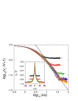
Figure 7: Log-log plot for the slip profiles. Here $v_{x}/V+1$ is the scaled slip velocity at the lower fluid-solid interface $z=0$, and $x/\sigma$ measures the distance from the MCL in units of $\sigma$. The wall is moving at $-V$, hence $v_{x}/V=0$ means complete slip and $v_{x}/V=-1$ means no slip. The $v_{x}$ profiles were obtained for five symmetric cases of Couette flow, which used different values for $H$ but the same value for $V$ ($=0.05\sqrt{\epsilon/m}$) and also the same parameters for densities and interactions. The symbols represent the MD results and the solid lines represent the continuum results, obtained for $H=6.8\sigma$ (black circles and line), $H=13.6\sigma$ (red squares and line), $H=27.2\sigma$ (green diamonds and line), $H=54.4\sigma$ (blue up-triangles and line), $H=68\sigma$ (orange down-triangles and line). There are two solid curves for each color, one for the slip profile left to the MCL and the other for that right to the MCL. The dashed line has the slope of $-1$, indicating that the $1/x$ behavior is approached for increasingly larger $H$. For $H=68\sigma$, the $1/x$ behavior extends from $|x|\approx 12\sigma\approx 6l_{s}$ to $50\sigma\approx 25l_{s}$, where $l_{s}$ was measured to be $2\sigma$. Inset: The scaled tangential velocity $v_{x}/V$ at $z=0$, plotted as a function of $x/\sigma$.

The continuum results shown in figure 7 were obtained on a uniform mesh, using the same set of parameter values corresponding to the same local properties in all the five MD simulations. We have extended the MCL simulations, through continuum hydrodynamics, to lower flow rates and much larger systems. For this purpose, we have employed the adaptive method based on iterative grid redistribution (Ren & Wang 2000). The computational mesh is redistributed following the behavior of the continuum solution so that fine molecular resolution is achieved in the interfacial region, while elsewhere a much coarser mesh is used to save computational cost. A semi-implicit time stepping scheme is also used to speed up the approach to steady state.

Figure 8: Log-log plot of the slip profiles. Here $v_{x}/V+1$ is the scaled slip velocity at the lower fluid-solid interface $z=0$, and $x/l_{s}$ measures the distance from the MCL in unit of $l_{s}$. The wall is moving at $-V$, hence $v_{x}/V=0$ means complete slip and $v_{x}/V=-1$ means no slip. There are three symmetric cases of Couette flow. The black solid line denotes the case of $H=326\sigma$, $V=0.005\sqrt{\epsilon/m}$ and $l_{s}=1.24\sigma$, the red dashed line denotes the case of $H=326\sigma$, $V=0.0025\sqrt{\epsilon/m}$ and $l_{s}=1.24\sigma$, and the blue dotted line denotes the case of $H=326\sigma$, $V=0.0025\sqrt{\epsilon/m}$ and $l_{s}=0.62\sigma$. The green dot-dashed line has the slope of $-1$, indicating a $1/x$ region much wider than that in figure 7. Inset: Universal slip profile. The scaled tangential velocity $v_{x}/V$ at $z=0$ is plotted as a function of the scaled coordinate $x/l_{s}$ for the three cases. The slip profiles exhibit a partial-slip region as large as hundreds of $l_{s}$. The relation $v_{x}/V=1/(1+{|x|}/{2.14l_{s}})-1$ is also plotted by the orange dot-dashed line, showing an extremely good fit.

The continuum results for three large systems of low flow rates are shown in figure 8. The capillary force is verified to be important in the interfacial region only, whereas the pressure gradients and viscous forces show a much slower variation. They are balanced outside the interfacial region, and hence the flow is governed by the Stokes equation. This is expected, because the Reynolds number $m\rho VH/\eta\approx 0.6$ for $\rho\approx 0.8/\sigma^{3}$, $V=0.005\sqrt{\epsilon/m}$, $H\approx 300\sigma$, and $\eta\approx 2.0\sqrt{\epsilon m}/\sigma^{2}$. Figure 8 shows the slip profiles plotted on the log-log scale, which clearly exhibit the $1/x$ behavior extending from $|x|\approx 6l_{s}$ to $|x|\approx 270l_{s}$. The inset to figure 8 shows the scaled tangential velocity profiles at the solid surface, from which the existence of a universal slip profile is evident. Physically, when $H\gg l_{s}$, the Stokes flow is governed by only one velocity scale $V$ and one length scale $l_{s}$. Thus universality becomes evident from $v_{x}/V$ plotted as a function of $x/l_{s}$. A heuristic account of the universal slip profile is as follows. Away from the MCL, the viscous shear stress is given by $-a\eta v_{x}(x)/|x|$, where $a$ is a constant $\sim 1$ and $v_{x}(x)$ is the local tangential velocity. The NBC implies $v_{x}^{slip}(x)=-al_{s}v_{x}(x)/|x|$. Combining this equation with $v_{x}^{slip}=v_{x}+V$ yields $v_{x}^{slip}(x)/V=1/(1+{|x|}/{al_{s}})$. This relation, with $a\approx 2.14$ for best fit, agrees with the continuum slip profiles extremely well, as seen in the inset to figure 8.

5 Scaling analysis: sharp or diffusive interface limit

In this section we look at the MCL problem from two different perspectives. These naturally arise from the physical reality that there are two distinct regions in the MCL problem: the interfacial region and the rest. In the perspective of the sharp interface limit, the problem is looked at from outside the interfacial region. The effect of the interfacial region is taken into account only in an integrated sense. In the diffuse interface limit, on the other hand, we examine the problem when the interfacial region is physically large. It turns out that the two limits can be mathematically analyzed by varying the magnitude of $M$ and $\Gamma$. In addition, we also give an abbreviated account of the recent work by ? on the sharp interface limit, which not only simplifies the mathematics, but also expresses the GNBC without the $\phi$ variable, and hence physically more transparent.

In appendix B we have derived the total rate of energy dissipation in steady state (see equations (B 56), (B 57), and (B 58)),

$$\begin{array}[]{lll}R_{2}\left[{\bf v}\right]&=&R_{v}\left[{\bf v}\right]+R_{s}\left[{\bf v}\right]+R_{d}\left[{\bf v}\right]+R_{r}\left[{\bf v}\right]\\ &=&\int d{\bf r}\left[\displaystyle\frac{\eta}{2}(\partial_{i}v_{j}+\partial_{j}v_{i})^{2}\right]+\int dS\left[\beta\left(v_{\tau}^{slip}\right)^{2}\right]+\\ &&\int d{\bf r}_{1}d{\bf r}_{2}\left[-\displaystyle\frac{1}{M}G({\bf r}_{1},{\bf r}_{2})\left({\bf v}\cdot\nabla\phi\right)_{{\bf r}_{1}}\left({\bf v}\cdot\nabla\phi\right)_{{\bf r}_{2}}\right]+\int dS\left[\displaystyle\frac{1}{\Gamma}\left(v_{\tau}\partial_{\tau}\phi\right)^{2}\right].\end{array}$$ (5.45)

This function(al) is useful to the variational analysis of the sharp/diffuse interface limits. It is obtained by eliminating the two rates $({\bf J},\dot{\phi})$ by expressing them in $\bf v$, for the steady state. The Stokes equation (3.31) and the GNBC (3.32) can be derived by minimizing $R_{2}[{\bf v}]$ with respect to $\bf v$, supplemented with equations (3.29) and (3.30) for the linear dissipative dynamics of $\phi$ (see equations (B 61) and (B 62)).

The CH diffuse-interface modeling allows diffusive transport through the fluid-fluid interface (Seppecher 1996; Jacqmin 2000; Chen, Jasnow & Vinals 2000; Pismen & Pomeau 2000; Briant & Yeomans 2004). By taking the limit of $M\to 0$ and $\Gamma\to 0$, we obtain the sharp interface limit in which advection dominates such that $\dot{\phi}\to 0$ and ${\partial\phi}/{\partial t}\to-{\bf v}\cdot\nabla\phi$. According to equation (5.45), if $1/M$ and $1/\Gamma$ both approach positive infinity, minimizing $R_{2}$ with respect to $\bf v$ then requires ${\bf v}\cdot\nabla\phi\to 0$ in the interfacial region (see the last two terms on the right-hand side of equation (5.45)). That means in steady state the flow is parallel to the interface.

The limiting magnitude of ${\bf v}\cdot\nabla\phi$ can be obtained through a scaling analysis. We assume that the interfacial thickness $\xi$ is much smaller than the smallest interfacial curvature radius, a limit realized for moderate shear rates. Integrating the Stokes equation (3.31) across the fluid-fluid interface yields $|\mu|\phi_{+}\sim\eta||\nabla{\bf v}||$, from which we have $|\mu|\sim\eta V/l\phi_{+}$, where $V$ and $l$ are the characteristic velocity and length scales of the flow. Integrating equation (3.29) (with ${\partial\phi}/{\partial t}=0$ in steady state) across the fluid-fluid interface yields $|v_{m}|\phi_{+}\sim M||\nabla\mu||$, from which we have $|v_{m}|\sim M|\mu|/l\phi_{+}$, where $v_{m}$ is the velocity component along the interfacial normal $m$. Together, $|\mu|\sim\eta V/l\phi_{+}$ and $|v_{m}|\sim M|\mu|/l\phi_{+}$ lead to $|v_{m}|/V\sim M\eta/l^{2}\phi_{+}^{2}$ for the dimensionless interfacial normal velocity. This relation indicates that in order to realize the sharp interface limit, $\sqrt{M\eta}/\phi_{+}$ is the length scale which must be made small enough compared to $l$. (This length scale arises from the coupling of equations (3.31) and (3.29) (Bray 1994; Jacqmin 2000).) As for the characteristic length $l$ of the flow field, it is given by the slip length $l_{s}$ in the inner region close to the contact line, where $l_{s}$ is actually the only length scale governing the Stokes flow. Far away from the contact line, $l$ becomes the dimension of the confined system, e.g., $l\sim H$. Typically $l_{s}$ is much smaller than $H$, and consequently $|v_{m}|$ reaches the maximum in the immediate vicinity of the MCL. This leads to the first conclusion that the sharp interface limit is realized in the bulk when

$$\frac{|v_{m}|}{V}\sim\displaystyle\frac{M\eta}{l_{s}^{2}\phi_{+}^{2}}\ll 1.$$ (5.46)

This relation ensures the flow to be parallel to the interface in the inner region of fast velocity variation and large interfacial curvature.

In the sharp interface limit, the tangential viscous stress is vanishingly small at the MCL because of the vanishing interfacial normal velocity there. Here we consider the case of $\theta_{s}=90^{\circ}$ for simplicity and generalization to $\theta_{s}\neq 90^{\circ}$ is straightforward. It follows that in steady state the near-complete slip at the MCL is mainly sustained by the uncompensated Young stress: $\beta V\sim\gamma\cos\theta_{d}/\xi$, where $V$ is for the maximum slip velocity (the wall speed relative to the stationary fluid-fluid interface) and $\gamma\cos\theta_{d}/\xi$ is obtained by considering the integrated uncompensated Young stress in equation (4.43) as distributed within $\xi$. The difference between the dynamic and static contact angles, $\Delta\theta=\theta_{s}-\theta_{d}$, is then obtained as $\Delta\theta\sim\xi\beta V/\gamma=\xi Ca/l_{s}$, where $l_{s}=\eta/\beta$ is the slip length and $Ca=\eta V/\gamma$ is the capillary number. Integrating equation (3.30) (with ${\partial\phi}/{\partial t}=0$) across the fluid-fluid interface along the solid surface yields the tangential velocity across the interface $|v_{\tau}|\sim\Gamma K\cos\theta_{d}\approx\Gamma K\Delta\theta$. (For $\theta_{s}=90^{\circ}$, the tangential direction $\tau$ is the same as the interfacial normal $m$, and hence $v_{\tau}$ becomes $v_{m}$.) Substituting $\Delta\theta\sim\xi Ca/l_{s}$ into $|v_{m}|\sim\Gamma K\Delta\theta$, we obtain $|v_{m}|\sim\Gamma K\xi Ca/l_{s}$, and hence $|v_{m}|/V\sim\Gamma K\xi\eta/\gamma l_{s}$. Using $\gamma=2\sqrt{2}K\phi_{+}^{2}/3\xi$, we obtain ${|v_{m}|}/{V}\sim{\Gamma\xi^{2}\eta}/{\phi_{+}^{2}l_{s}}$. This leads to the second conclusion that the sharp interface limit is realized at the contact line when

$$\frac{|v_{m}|}{V}\sim\displaystyle\frac{\Gamma\xi^{2}\eta}{\phi_{+}^{2}l_{s}}\ll 1,$$ (5.47)

which ensures the interface not to be penetrated by the flow. Note that the two conditions (5.46) and (5.47) are independent of the magnitude of $V$. This is consistent with the linearity of the hydrodynamic model (for sufficiently low flow rates) and has been well verified numerically.

In Sec. 4, it has been mentioned that $M$ and $\Gamma$ are treated as fitting parameters to optimize the MD-continuum comparison. Since the fluid-fluid interface in our MD simulations is impenetrable, the hydrodynamic model has to be within the sharp interface limit in order to reproduce the MD results. It follows that the values of $M$ and $\Gamma$ must satisfy the conditions (5.46) and (5.47). Moreover, as long as the sharp interface limit is reached, the continuum predictions are not sensitive to the values of $M$ and $\Gamma$. Such has indeed been our experience. That means $M$ and $\Gamma$ should not be regarded as fitting parameters in our MD-continuum comparison because they are simply used to realize the sharp interface limit, in accordance with the interface impenetrability conditions (viewed outside the interfacial region).

We have shown that in order to sustain the near-complete slip at the MCL, the dynamic contact angle $\theta_{d}$ has to deviate from the static angle $\theta_{s}$ by $\Delta\theta\sim\xi Ca/l_{s}$. A similar scaling relation has recently been obtained by ? in a general discussion on the sharp interface limit of the GNBC. Here we derive a complete expression for $\Delta\theta$ within the CH phase-field formulation. Consider an interface deformed by the shearing movement of confining walls (see figure 2b). In steady state the tangential viscous stress is negligibly small at the MCL where the slip is near-complete ($v_{x}^{slip}\approx V$ at the lower fluid-solid interface). Therefore the GNBC may be expressed as $\beta V=-K\partial_{z}\phi\partial_{x}\phi$. Suppose the deviation of $\theta_{d}$ from $\theta_{s}=90^{\circ}$ is very small (this is indeed the case, as we will show later). Then $\partial_{z}\phi\approx-\partial_{x}\phi\cos\theta_{d}$ and $\beta V\approx K\left(\partial_{x}\phi\right)^{2}\cos\theta_{d}$. Using the interfacial profile $\phi(x)=\phi_{+}\tanh\left(x/{\sqrt{2}\xi}\right)$ at $z=0$ (for a gently deformed interface), we obtain $\beta V\approx{K\phi_{+}^{2}}\cos\theta_{d}/{2\xi^{2}}$. It follows that

$$\Delta\theta=\displaystyle\frac{4\sqrt{2}}{3}\displaystyle\frac{\xi}{l_{s}}\displaystyle\frac{\eta V}{\gamma}.$$ (5.48)

This expression has been quantitatively verified. Substituting the MD values $l_{s}=3.8\xi$, $\gamma=5.5\epsilon/\sigma^{2}$, $\eta=1.95\sqrt{\epsilon m}/\sigma^{2}$, and $V=0.25\sqrt{\epsilon/m}$ into equation (5.48) yields $\Delta\theta=0.044$ (or $2.5^{\circ}$), in excellent agreement with $\cos\theta_{d}=0.0437$ obtained from the $\phi=0$ locus in the continuum solution. Actually there is another measure of $\cos\theta_{d}$ using the integrated Young stress $\int_{int}dxK\partial_{n}\phi\partial_{x}\phi=\gamma\cos\theta_{d}$, which produces a value only slightly different from that determined by the $\phi=0$ locus. We note that in our nanoscale MD simulations, $l_{s}$ is typically larger than $\xi$ and $\gamma>10\eta V$, and hence $\Delta\theta<0.1$. Yet this small angle of deviation is necessary for the uncompensated Young stress to sustain the near-complete slip of the MCL (Qian, Wang & Sheng 2003).

In a recent study of the sharp interface limit of the GNBC by ?, it has been shown that the deviation of the dynamic contact angle $\theta_{d}$ from the static contact angle $\theta_{s}$ is proportional to the dimensionless parameter $\beta^{*}V\delta/\gamma$, which measures the relative strength of the frictional force between the fluid and the solid and the interfacial force between the fluids. Here $\beta^{*}$ is the (average) slip coefficient in the contact line region, depending on $\beta_{1}$ and $\beta_{2}$ in the two single-phase flow regions as well as the fluid-fluid interfacial structure, and $\delta$ is the fluid-fluid interfacial thickness. Numerical results have been obtained for the relation between the microscopic contact angle $\theta_{d}$ and the apparent contact angle, demonstrating good agreement with the analytical results based on matched asymptotic expansions (Cox 1986).

From the above, it follows that in the sharp interface limit the contact angle can be set at the value of the static contact angle (for $\xi\to 0$ and/or $Ca\to 0$), and since outside the fluid-fluid interfacial region the NBC is valid, numerically the flow field can be calculated separately on the two sides of the interface, linked together via the interface transition relations (zero normal component of velocity, continuity of tangential component of velocity, continuity of tangential stress, normal stress difference across the interface being balanced by the tensile force proportional to the interface curvature) (Zhou & Sheng 1990; Ren & E 2005b). However, in such numerical solutions the tangential (viscous) stress is necessarily discontinuous at the contact line. This can be clearly seen by considering the tangential viscous stresses approached along the three interfaces (two fluid-solid and one fluid-fluid) terminating at the contact line. For simplicity, let us consider a fluid-fluid interface vertically intersecting the solid surface. Velocity continuity dictates that the tangential viscous stress at the solid surface approaches $\beta_{1}V$ (or $\beta_{2}V$) at the contact line in the single-phase flow region left (or right) to the fluid-fluid interface, with $\beta_{1}$ and $\beta_{2}$ being the slip coefficients in the left and right regions, respectively. However, the impenetrability condition at the fluid-fluid interface dictates that along this interface, the velocity component parallel to the solid surface vanishes, leading to a vanishing tangential viscous stress at the solid surface when approached along the fluid-fluid interface down to the contact line. Hence there exist three distinct values for the tangential viscous stress. The uncompensated Young stress thus enters as the required subsidiary condition to complete the picture and make the solutions physically meaningful. In particular, the uncompensated Young stress interpolates between the two values of $\beta_{1}V$ and $\beta_{2}V$, with a mean value given by $(\beta_{1}+\beta_{2})V/2$, if the two fluids are assumed to interact with the solid independently (Qian, Wang & Sheng 2003).

Opposite to the sharp interface limit is the limit of $M\to\infty$ and $\Gamma\to\infty$. Obviously, in this limit minimizing $R_{2}$ in equation (5.45) is equivalent to minimizing $R_{1}$ in equation (3.8) because $R_{d}$ and $R_{r}$ both vanish regardless of the velocity distribution (see equations (B 56) and (B 57)). As a consequence, the flow field and the fluid-fluid interface are decoupled: the velocity is distributed as if there is only one single phase while the interfacial profile approaches the equilibrium one. As the fluid-fluid interface becomes very transparent (through diffusive transport), the contact line loses its usual implications. Indeed, it has been shown that as this limit is approached, the stress singularity can be lifted even if the no-slip boundary condition is applied (Seppecher 1996; Jacqmin 2000; Chen, Jasnow & Vinals 2000; Briant & Yeomans 2004). This result can be made intuitively plausible from our variational formulation as follows.

According to equation (5.45), if the functional $R_{2}[{\bf v}]$ is to be minimized subject to $\beta$, $1/M$, and $1/\Gamma$ all approaching positive infinity, then the problem is reduced to solving the Stokes equation subject to the no-slip boundary condition $v_{\tau}^{slip}=0$ and the interface impenetrability condition $v_{m}=0$. This leads to the well-known non-integrable singularity in viscous dissipation. Therefore, mathematically the contact-line singularity may be viewed as resulting from minimizing $R_{2}[{\bf v}]$ with $\beta$, $1/M$, and $1/\Gamma\to\infty$. By removing either the $\beta\to\infty$ constraint (i.e., allowing slipping), or the $1/M$, $1/\Gamma\to\infty$ constraint (i.e., allowing diffusive relaxation), the total dissipation can only decrease from infinity, thus regularizing the solution. This is especially the case since the divergence is logarithmic in nature, i.e., the divergence is only marginal. We should note, however, that physically realistic cases correspond to $\beta$, $1/M$, and $1/\Gamma$ all remain finite, as evidenced by MD results. In fact, application of the above considerations to the problem of corner-flow singularity (involving a flow in a corner with one rigid plane sliding over another) (Batchelor 1991; Moffatt 1964; Koplik & Banavar 1995) would be equally valid (Qian & Wang 2005).

It is interesting to note that in either of the two limits discussed above, the rate of interfacial dissipation, $R_{d}+R_{r}$, tends to vanish. In the sharp interface limit of $M\to 0$ and $\Gamma\to 0$, the limiting behaviors of the interfacial normal velocity expressed in equations (5.46) and (5.47) make $R_{d}\sim M$ and $R_{r}\sim\Gamma$. (Equation (B 56) indicates $R_{d}\propto|v_{m}|^{2}/M$ while equation (5.46) indicates $|v_{m}|\propto M$, and hence $R_{d}\propto M\to 0$. Similarly, $R_{r}\propto\Gamma\to 0$.) In the opposite limit of $M\to\infty$ and $\Gamma\to\infty$, as the interface is penetrated by the flow, $R_{d}$ and $R_{r}$ simply vanish as $1/M$ and $1/\Gamma$, respectively. That the positive definite rate of interfacial dissipation, $R_{d}+R_{r}$, approaches zero in the two opposite limits implies that a maximum should be reached somewhere in between. However, the total rate of dissipation $R_{2}$ should increase monotonically from the limit of $M\to\infty$ and $\Gamma\to\infty$ to that of $M\to 0$ and $\Gamma\to 0$. Although there is only $R_{v}+R_{s}$ left for $R_{2}$ in either of the two limits, the latter (sharp interface) limit imposes vanishing interfacial normal velocity as the additional condition. This would certainly lead to a flow whose total rate of dissipation is larger than that obtained from minimizing the same functional without the additional constraint.

We want to point out that while mathematically the sharp interface limit may be simply obtained by excluding $R_{d}$ and $R_{r}$ from $R_{2}$ and applying $v_{m}=0$ at the interface instead, physically the two-phase interfacial dissipation may not always be negligible, especially when the interfacial region of partial miscibility has finite and non-negligible width such that structural relaxation may occur.

It should be noted that dimensional analysis indicates that $\left[M\right]=\left[\Gamma\right]\left[{\rm Length}\right]^{3}$, i.e., there is a length scale $l_{0}$ which links these two parameters through the relation $M=\Gamma l_{0}^{3}$. Physically it is plausible to assume that $l_{0}$ is determined by a combination of microscopic factors, such as fluid-fluid interaction, fluid-solid interaction, molecular organization of the fluids, and molecular structure of the wall. Hence $M$ and $\Gamma$ may be physically related in any given system.

6 Concluding remarks

We should point out the inadequacies in our present formulation. First, the free energy used to delineate the two fluids is a minimal model. It neglects, for example, the density variation that can be fairly significant in the interfacial region. Second, our model in its present form is only applicable to simple liquids. Complex fluids would require nontrivial extensions. Third, we have neglected the van der Waals interaction which is very important in understanding precursor films. These and other inadequacies represent tasks still to be pursued. The main purpose of this paper is to outline the framework of a general theory which can resolve the MCL problem in its simplest form.

It is important to emphasize that while the partial slip in single-phase flows is generally small and quantitatively indistinguishable from no-slip, yet its significance is qualitatively much greater. First, it is clear from the above that the GNBC goes hand-in-hand with the NBC in single-phase flows, and that it is incompatible with the no-slip boundary condition even in single-phase flows. The latter is clear from the power-law partial slip which extends mesoscopic distances into single-phase flow regimes. Second, even if the slip is small, the fact that slip exists means that its magnitude may be manipulated, i.e., it can be made larger or smaller. In particular, since the slip coefficient is a thermodynamic quantity, just as the viscosity, its magnitude should depend on molecular interactions and interface geometries (as well as the state variables such as temperature) (Barrat & Bocquet 1999b; Leger 2003; Granick, Zhu & Lee 2003; Zhu & Granick 2004; Neto et al. 2005), a fact which can be used to advantage experimentally through nanoscale manipulations and environmental controls. For example, effective slip at nano-patterned surfaces has already been studied (Philip 1972; Lauga & Stone 2003; Cottin-Bizonne et al. 2003; Cottin-Bizonne et al. 2004; Priezjev, Darhuber & Troian 2005; Qian, Wang & Sheng 2005). In contrast, no-slip boundary condition is a clean-cut statement, with no room for adjustment or for physics considerations, only carries with it the burden of proof. Here the broad applicability of the no-slip boundary condition can not be considered as proof against slipping, as a very small amount of partial slip would clearly lead to similar results. It is therefore rather obvious that whereas slip/partial-slip can be derived from general principles and demonstrated through MD simulations, no-slip has yet to be proved with similar generalities. In fact, at present slip is already a subject with some fairly extensive literature. We refer to the reviews by ? and by ? for a more complete list of references.

In closing, we note that in the case of the moving contact line, complete slip occurs in the linear regime (i.e., $\beta$ is a constant). This is in contrast to the view that complete slip can only occur when “interface fracturing” occurs, i.e., in the fully nonlinear regime (sometimes also denoted as “super slipping” or “threshold slipping”), corresponding to a stress-dependent $\beta$ (see e.g. Thompson & Troian 1997). It is rather likely that a statistical mechanical study of the slip coefficient can indeed produce a threshold behavior, e.g., $\beta$ approaches zero as the shear stress exceeds a certain threshold. However, in the linear regime this is not the case. The difference between the MCL complete slip and the interface fracturing is that in the case of MCL, the (complete) slip velocity can be very small and the relevant shear stress can be low. The fact that complete slip can occur in this case is due to the localized nature of the uncompensated Young stress, in addition to the tangential viscous stress. Thus we can have complete slip in both the linear and nonlinear regimes, with different underlying physics.

The authors are grateful to Weinan E, Chun Liu and Weiqing Ren for helpful discussions. This work was partially supported by the Hong Kong RGC CERG No. 604803, the RGC central allocation grant CA05/06.SC01, and the Croucher Foundation Grant Z0138.

A The principle of minimum energy dissipation

To outline the principle of minimum energy dissipation (Onsager 1931a and 1931b), consider a system described by one single variable $\alpha$, governed by the overdamped Langevin equation

$$\gamma\dot{\alpha}=-\displaystyle\frac{\partial F(\alpha)}{\partial\alpha}+\zeta(t),$$ (A 49)

where $\gamma$ is the frictional coefficient, $\dot{\alpha}$ is the rate of change of $\alpha$, $F(\alpha)$ is the free energy, and $\zeta(t)$ is a white noise satisfying $\langle\zeta(t)\zeta(t^{\prime})\rangle=2\gamma k_{B}T\delta(t-t^{\prime})$, with $k_{B}$ denoting the Boltzmann constant and $T$ the temperature. The probability of finding the system in the state described by $\alpha$ is a function of time, denoted by $P(\alpha,t)$ and governed by the Fokker-Planck equation

$$\frac{\partial P}{\partial t}=D\left[\displaystyle\frac{\partial^{2}P}{\partial\alpha^{2}}+\displaystyle\frac{1}{k_{B}T}\displaystyle\frac{\partial}{\partial\alpha}\left(\displaystyle\frac{\partial F}{\partial\alpha}P\right)\right],$$ (A 50)

where $D$ is the diffusion coefficient satisfying the Einstein relation $\gamma D=k_{B}T$. It is clear that the Boltzmann distribution $P_{eq}(\alpha)\propto\exp\left[-F(\alpha)/k_{B}T\right]$ is a stationary solution of the Fokker-Planck equation (A 50). It can be shown (Langer 1968) that the transition probability from $\alpha$ at $t$ to $\alpha^{\prime}$ at $t+\Delta t$, i.e., $P_{2}(\alpha^{\prime},t+\Delta t;\alpha,t)$, is given by

$$P_{2}(\alpha^{\prime},t+\Delta t;\alpha,t)=\displaystyle\frac{1}{\sqrt{4\pi D\Delta t}}\exp\left[-\displaystyle\frac{(\alpha^{\prime}-\alpha)^{2}}{4D\Delta t}\right]\exp\left[-\displaystyle\frac{F(\alpha^{\prime})-F(\alpha)}{2k_{B}T}\right],$$ (A 51)

for $\alpha^{\prime}$ in the vicinity of $\alpha$ and short time interval $\Delta t$. The most probable transition occurs between $\alpha$ and $\alpha^{\prime}$ is the one which minimizes

$$A=\displaystyle\frac{\gamma(\alpha^{\prime}-\alpha)^{2}}{2\Delta t}+\left[F(\alpha^{\prime})-F(\alpha)\right]\approx\left[\displaystyle\frac{\gamma}{2}\dot{\alpha}^{2}+\displaystyle\frac{\partial F(\alpha)}{\partial\alpha}\dot{\alpha}\right]\Delta t,$$ (A 52)

Here $\dot{\alpha}=(\alpha^{\prime}-\alpha)/\Delta t$ and the minimum of $A$ is taken with respect to $\alpha^{\prime}$, or equivalently $\dot{\alpha}$, for prescribed $\alpha$. The Euler-Lagrange equation for minimizing $A$ is thus

$$\gamma\dot{\alpha}=\displaystyle\frac{\gamma(\alpha^{\prime}-\alpha)}{\Delta t}=-\displaystyle\frac{\partial F(\alpha)}{\partial\alpha},$$ (A 53)

as expected from the Langevin equation (A 49). Equation (A 53) is actually the simplest, one-variable version of the linear relation in equation (3.1) for rates and forces, and the function $\gamma\dot{\alpha}^{2}/2+(\partial F/\partial\alpha)\dot{\alpha}$ in $A$ is the corresponding one-variable version of the function $\Phi(\dot{\alpha},\dot{\alpha})+\dot{F}(\alpha,\dot{\alpha})$ in Onsager’s variational principle, stated by equations (3.2), (3.3), and (3.4). From the above discussion, it is clear that (1) the variation of $A$ should be taken with respect to the rate $\dot{\alpha}$, for prescribed state variable $\alpha$, (2) the minimum dissipation principle implies the balance of dissipative force and the force derived from free energy (see equation (A 53)), and (3) the minimum dissipation principle yields the most probable course of a dissipative process, provided the displacement from the equilibrium is small (Onsager 1931b, Onsager & Machlup 1953).

B The dissipation function in steady state

In a steady state with ${\partial\phi}/{\partial t}=0$, the total rate of energy dissipation $R_{2}=2\Phi$ in equations (3.21) and (3.22) can be expressed as a functional of ${\bf v}({\bf r})$ only. This is because for prescribed phase field $\phi$, the rate $\bf J$ in the bulk can be determined from $\dot{\phi}={\bf v}\cdot\nabla\phi$ through equations (3.28) and (3.29) while the rate $\dot{\phi}=v_{\tau}\partial_{\tau}\phi$ at the solid surface is already given in terms of ${\bf v}$. By expressing $R_{2}$ as a functional of ${\bf v}({\bf r})$, we can obtain a form of the dissipation function that is useful to the variational analysis of the sharp interface limit and the diffuse interface limit.

From equation (3.29) with ${\partial\phi}/{\partial t}=0$, we can formally express $\mu({\bf r})$ by

$$\mu({\bf r})=\displaystyle\frac{1}{M}\int d{\bf r}^{\prime}G({\bf r},{\bf r}^{\prime})\left({\bf v}\cdot\nabla\phi\right)_{{\bf r}^{\prime}},$$ (B 54)

where $G({\bf r},{\bf r}^{\prime})$ is the Green function for the Laplacian operator satisfying the boundary condition $\partial_{n}\mu=0$ at the solid surface. From $R_{d}$ in equation (3.19) and $J=-M\nabla\mu$ (equation (3.28)), we have

$$R_{d}=\int d{\bf r}\left[M(\nabla\mu)^{2}\right]=\int d{\bf r}\left[-M\mu\nabla^{2}\mu\right],$$ (B 55)

where the integration by parts has been used with $\partial_{n}\mu=0$ at the solid surface. Substituting equation (B 54) into (B 55) yields

$$R_{d}\left[{\bf v}\right]=\int d{\bf r}_{1}d{\bf r}_{2}\left[-\displaystyle\frac{1}{M}G({\bf r}_{1},{\bf r}_{2})\left({\bf v}\cdot\nabla\phi\right)_{{\bf r}_{1}}\left({\bf v}\cdot\nabla\phi\right)_{{\bf r}_{2}}\right].$$ (B 56)

Meanwhile, substituting $\dot{\phi}=v_{\tau}\partial_{\tau}\phi$ into $R_{r}$ in equation (3.20), we obtain

$$R_{r}\left[{\bf v}\right]=\int dS\left[\displaystyle\frac{1}{\Gamma}\left(v_{\tau}\partial_{\tau}\phi\right)^{2}\right].$$ (B 57)

Combining equations (3.9), (3.10), (B 56), and (B 57) with $R_{2}$ defined in equations (3.21) and (3.22), we obtain

$$\begin{array}[]{lll}R_{2}\left[{\bf v}\right]&=&R_{v}\left[{\bf v}\right]+R_{s}\left[{\bf v}\right]+R_{d}\left[{\bf v}\right]+R_{r}\left[{\bf v}\right]\\ &=&\int d{\bf r}\left[\displaystyle\frac{\eta}{2}(\partial_{i}v_{j}+\partial_{j}v_{i})^{2}\right]+\int dS\left[\beta\left(v_{\tau}^{slip}\right)^{2}\right]+\\ &&\int d{\bf r}_{1}d{\bf r}_{2}\left[-\displaystyle\frac{1}{M}G({\bf r}_{1},{\bf r}_{2})\left({\bf v}\cdot\nabla\phi\right)_{{\bf r}_{1}}\left({\bf v}\cdot\nabla\phi\right)_{{\bf r}_{2}}\right]+\int dS\left[\displaystyle\frac{1}{\Gamma}\left(v_{\tau}\partial_{\tau}\phi\right)^{2}\right],\end{array}$$ (B 58)

for the total rate of dissipation in two-phase flows, which is the sum of $R_{v}$ due to viscosity, $R_{s}$ due to slipping, $R_{d}$ due to diffusion in the bulk, and $R_{r}$ due to relaxation at the surface.

In accordance with the principle of minimum energy dissipation (Onsager 1931a and 1931b), for steady state the equation(s) of motion can be derived from minimizing the dissipation-function $\Phi$ ($=\frac{1}{2}R_{2}$ here) with respect to the rates. Here we note that in steady state, the rates $\bf J$ in the bulk and $\dot{\phi}$ at the solid surface are already determined by $\bf v$ for prescribed $\phi$, and $R_{2}[{\bf v}]$ in equation (B 58) displays a symmetric, quadratic form as a function(al) of $\bf v$, in accordance with the reciprocal relations, i.e., $\rho_{ij}=\rho_{ji}$ for the coefficients $\rho_{ij}$ in $\Phi(\dot{\alpha},\dot{\alpha})=\frac{1}{2}\sum_{i,j}\rho_{ij}\dot{\alpha}_{i}\dot{\alpha}_{j}$ (equation (3.3)). The variation of the total dissipation $R_{2}[{\bf v}]$ should be taken with respect to $\bf v$ only, as it is the only rate.

Based on equation (B 58), minimizing $R_{2}$ with respect to ${\bf v}$ in the bulk yields the Stokes equation (3.31), while minimizing $R_{2}$ with respect to tangential fluid velocity $v_{\tau}$ at the solid surface yields the GNBC (3.32). That is, consider a variation of the velocity field ${\bf v}({\bf r})\to{\bf v}({\bf r})+\delta{\bf v}({\bf r})$. The associated changes in $R_{v}$ and $R_{s}$ are already given by equations (3.11) and (3.12), and those in $R_{d}[{\bf v}]$ and $R_{r}[{\bf v}]$ are given by

$$\delta R_{d}=\int d{\bf r}d{\bf r}^{\prime}\left[-\displaystyle\frac{2G({\bf r},{\bf r}^{\prime})\left({\bf v}\cdot\nabla\phi\right)_{{\bf r}^{\prime}}\left(\delta{\bf v}\cdot\nabla\phi\right)_{{\bf r}}}{M}\right]=-2\int d{\bf r}\left[\mu\partial_{i}\phi\delta v_{i}\right],$$ (B 59)

and

$$\delta R_{r}=\int dS\left[\displaystyle\frac{2}{\Gamma}\left(v_{\tau}\partial_{\tau}\phi\right)\delta v_{\tau}\partial_{\tau}\phi\right]=-2\int dS\left[L(\phi)\partial_{\tau}\phi\delta v_{\tau}\right],$$ (B 60)

where equations (3.29) and (3.30) have been used. Combining equations (3.11), (3.12), (3.13), (B 59), and (B 60), we obtain the Euler-Lagrange equations

$$-2\eta\partial_{j}\left(\partial_{j}v_{i}+\partial_{i}v_{j}\right)-\partial_{i}\alpha-2\mu\partial_{i}\phi=0$$ (B 61)

in the bulk and

$$2\eta\left(\partial_{n}v_{\tau}+\partial_{\tau}v_{n}\right)+2\beta v_{\tau}^{slip}-2L(\phi)\partial_{\tau}\phi=0$$ (B 62)

at the surface. Note that equation (B 61) is identical to the Stokes equation (3.31) with $\partial_{j}v_{j}=0$ and $\alpha=-2p$, and equation (B 62) reduces to the GNBC (3.32).

References

- Barrat & Bocquet (1999a) Barrat, J-L. & Bocquet, L. 1999a Large slip effect at a nonwetting fluid-solid interface. Phys. Rev. Lett. 82, 4671-4674.
- Barrat & Bocquet (1999b) Barrat, J-L. & Bocquet, L. 1999b Influence of wetting properties on hydrodynamic boundary conditions at a fluid/solid interface. Faraday Discuss. 112, 119-128.
- Batchelor (1991) Batchelor, G.K. 1991 An introduction to fluid dynamics. Cambridge.
- Blake & Haynes (1969) Blake, T. D. & Haynes, J. M. 1969 Kinetics of liquid/liquid displacement. J. Colloid and Interface Sci. 30, 421-423.
- Bray (1994) Bray, A. J. 1994 Theory of phase-ordering kinetics. Adv. Phys. 43, 357-459.
- Briant & Yeomans (2004) Briant, A. J. & Yeomans, J. M. 2004 Lattice Boltzmann simulations of contact line motion. II. Binary fluids. Phys. Rev. E 69, 031603.
- Cahn & Hilliard (1958) Cahn, J. W. & Hilliard, J. E. 1958 Free energy of a nonuniform system. I. Interfacial free energy. J. Chem. Phys. 28, 258-267.
- Chella & Vinals (1996) Chella, R. & Vinals, J. 1996 Mixing of a two-phase fluid by cavity flow. Phys. Rev. E 53, 3832-3840.
- Chen, Jasnow & Vinals (2000) Chen, H. Y., Jasnow, D. & Vinals, J. 2000 Interface and contact line motion in a two phase fluid under shear flow. Phys. Rev. Lett. 85, 1686-1689.
- Cieplak, Koplik & Banavar (2001) Cieplak, M., Koplik, J. & Banavar, J. R. 2001 Boundary conditions at a fluid-solid interface. Phys. Rev. Lett. 86, 803-806.
- Cottin-Bizonne et al. (2003) Cottin-Bizonne, C., Barrat, J-L., Bocquet, L. & Charlaix, E. 2003 Low-friction flows of liquid at nanopatterned interfaces. Nat. Mater. 2, 237-240.
- Cottin-Bizonne et al. (2004) Cottin-Bizonne, C., Barentin, C., Charlaix, E., Bocquet, L. & Barrat, J-L. 2004 Dynamics of simple liquids at heterogeneous surfaces: Molecular-dynamics simulations and hydrodynamic description. Eur. Phys. J. E 15, 427-438.
- Cox (1986) Cox, R. G. 1986 The dynamics of the spreading of liquids on a solid surface. Part 1. Viscous flow. J. Fluid Mech. 168, 169-194.
- de Gennes (1985) De Gennes, P. G. 1985 Wetting: Statics and dynamics. Rev. Mod. Phys. 57, 827-863.
- Doi (1983) Doi, M. 1983 Variational principle for the Kirkwood theory for the dynamics of polymer solutions and suspensions. J. Chem. Phys. 79, 5080-5087.
- Dussan & Davis (1974) Dussan V., E. B. & Davis, S. H. 1974 On the motion of a fluid-fluid interface along a solid surface. J. Fluid Mech. 65, 71-95.
- Dussan (1976) Dussan V., E. B. 1976 The moving contact line: the slip boundary condition. J. Fluid Mech. 77, 665-684.
- Dussan (1979) Dussan V., E. B. 1979 On the spreading of liquids on solid surfaces: Static and dynamic contact lines. Ann. Rev. Fluid Mech. 11, 371-400.
- Edwards & Freed (1974) Edwards, S. F. & Freed, K. F. 1974 Theory of the dynamical viscosity of polymer solutions. J. Chem. Phys. 61, 1189-1202.
- Granick, Zhu & Lee (2003) Granick, S., Zhu, Y. & Lee, H. 2003 Slippery questions about complex fluids flowing past solids. Nat. Mater. 2, 221-227.
- Hadjiconstantinou (1999) Hadjiconstantinou, N. G. 1999 Hybrid atomistic–continuum formulations and the moving contact-line problem. J. Comput. Phys. 154, 245-265.
- Hocking (1977) Hocking, L. M. 1977 A moving fluid interface. Part 2. The removal of the force singularity by a slip flow. J. Fluid Mech. 79, 209-229.
- Huh & Mason (1977) Huh, C. & Mason, S. G. 1977 The steady movement of a liquid meniscus in a capillary tube. J. Fluid Mech. 81, 401-419.
- Hua & Scriven (1971) Hua, C. & Scriven, L. E. 1971 Hydrodynamic model of steady movement of a solid/liquid/fluid contact line. J. Colloid and Interface Sci. 35, 85-101.
- Jacqmin (2000) Jacqmin, D. 2000 Contact-line dynamics of a diffuse fluid interface. J. Fluid Mech. 402, 57-88.
- Koplik, Banavar & Willemsen (1988) Koplik, J., Banavar, J. R. & Willemsen, J. F. 1988 Molecular dynamics of Poiseuille flow and moving contact lines. Phys. Rev. Lett. 60, 1282-1285.
- Koplik, Banavar & Willemsen (1989) Koplik, J., Banavar, J. R. & Willemsen, J. F. 1989 Molecular dynamics of fluid flow at solid surfaces. Phys. Fluids A 1, 781-794.
- Koplik & Banavar (1995) Koplik, J. & Banavar, J. R. 1995 Corner flow in the sliding plate problem. Phys. Fluids 7, 3118-3125.
- Landau & Lifshitz (1997) Landau, L. D. & Lifshitz, E. M. 1997 Statistical Physics (Part 1). Oxford.
- Langer (1968) Langer, J. S. 1968 Theory of nucleation rates. Phys. Rev. Lett. 21, 973-976.
- Lauga & Stone (2003) Lauga, E. & Stone, H. A. 2003 Effective slip in pressure-driven Stokes flow. J. Fluid Mech. 489, 55-77.
- Leger (2003) Leger, L. 2003 Friction mechanisms and interfacial slip at fluid-solid interfaces. J. Phys.: Condens. Matter 15, S19-S29.
- Moffatt (1964) Moffatt, H. K. 1964 Viscous and resistive eddies near a sharp corner. J. Fluid Mech. 18, 1-18.
- Navier (1823) Navier, C. L. M. H. 1823 Memoire sur les lois du movement des fluides. Memoires de l’Academie Royale des Sciences de l’Institut de France 6, 389-440.
- Neto et al. (2005) Neto, C., Evans, D. R., Bonaccurso, E., Butt, H-J. & Craig, V. S. J. 2005 Boundary slip in Newtonian liquids: a review of experimental studies. Rep. Prog. Phys. 68, 2859-2897.
- Onsager (1931a) Onsager, L. 1931a Reciprocal relations in irreversible processes. I. Phys. Rev. 37, 405-426.
- Onsager (1931b) Onsager, L. 1931b Reciprocal relations in irreversible processes. II. Phys. Rev. 38, 2265-2279.
- Onsager & Machlup (1953) Onsager, L. & Machlup, S. 1953 Fluctuations and irreversible processes. Phys. Rev. 91, 1505-1512.
- Philip (1972) Philip, J. R. 1972 Integral properties of flows satisfying mixed no-slip and no-shear conditions. Z. Angew. Math. Phys. 23, 960-968.
- Pismen & Pomeau (2000) Pismen, L. M. & Pomeau, Y. 2000 Disjoining potential and spreading of thin liquid layers in the diffuse-interface model coupled to hydrodynamics. Phys. Rev. E 62, 2480-2492.
- Priezjev, Darhuber & Troian (2005) Priezjev, N. V., Darhuber, A. A. & Troian, S. M. 2005 Slip behavior in liquid films on surfaces of patterned wettability: Comparison between continuum and molecular dynamics simulations. Phys. Rev. E 71, 041608.
- Qian, Wang & Sheng (2003) Qian, T. Z., Wang, X. P. & Sheng, P. 2003 Molecular scale contact line hydrodynamics of immiscible flows. Phys. Rev. E 68, 016306.
- Qian, Wang & Sheng (2004) Qian, T. Z., Wang, X. P. & Sheng, P. 2004 Power-law slip profile of the moving contact line in two-phase immiscible flows. Phys. Rev. Lett. 93, 094501.
- Qian & Wang (2005) Qian, T. Z. & Wang, X. P. 2005 Driven cavity flow: From molecular dynamics to continuum hydrodynamics. SIAM Multiscale Model. Simul. 3, 749-763.
- Qian, Wang & Sheng (2005) Qian, T. Z., Wang, X. P. & Sheng, P. 2005 Hydrodynamic slip boundary condition at chemically patterned surfaces: A continuum deduction from molecular dynamics. Phys. Rev. E 72, 022501.
- Rayleigh (1873) Rayleigh, Lord 1873 Some general theorems relating to vibrations. Proc. Math. Soc. London 4, 357-368.
- Ren & Wang (2000) Ren, W. & Wang, X. P. 2000 An iterative grid redistribution method for singular problems in multiple dimensions. J. Comput. Phys. 159, 246-273.
- Ren & E (2005a) Ren, W. & E, W. 2005a Heterogeneous multiscale method for the modeling of complex fluids and micro-fluidics. J. Comput. Phys. 204, 1-26.
- Ren & E (2005b) Ren, W. & E, W. 2005b Boundary conditions for the moving contact line problem. preprint.
- Seppecher (1996) Seppecher, P. 1996 Moving contact lines in the Cahn-Hilliard theory. Int. J. Engng. Sci. 34, 977-992.
- Thompson & Robbins (1989) Thompson, P. A. & Robbins, M. O. 1989 Simulations of contact-line motion: Slip and the dynamic contact angle. Phys. Rev. Lett. 63, 766-769.
- Thompson & Robbins (1990) Thompson, P. A. & Robbins, M. O. 1990 Shear flow near solids: Epitaxial order and flow boundary conditions. Phys. Rev. A 41, 6830-6837.
- Thompson, Brinckerhoff & Robbins (1993) Thompson, P. A., Brinckerhoff, W. B. & Robbins, M. O. 1993 Microscopic studies of static and dynamic contact angles. J. Adhesion Sci. Tech. 7, 535-554.
- Thompson & Troian (1997) Thompson, P. A. & Troian, S. M. 1997 A general boundary condition for liquid flow at solid surfaces. Nature 389, 360-362.
- Zhou & Sheng (1990) Zhou, M. Y. & Sheng, P. 1990 Dynamics of immiscible-fluid displacement in a capillary tube. Phys. Rev. Lett. 64, 882-885.
- Zhu & Granick (2004) Zhu, Y. & Granick, S. 2004 Superlubricity: A paradox about confined fluids resolved. Phys. Rev. Lett. 93, 096101.