Nonequilibrium phase transitions
in a quasi-two-dimensional superlattice
with parabolic miniband

Abstract

Distribution function and current density in a one-dimensional superlattice with parabolic miniband are calculated. The current dependence on the temperature coincides with experimental data. Generalization is carried out to quasi-two-dimensional superlattice with paraboloidal miniband. For a sample opened in $Y$ direction with dc current in $X$ direction, a novel nonequilibrium phase transition is found, namely, appearing a spontaneous transverse electric field $E_{y}$ under temperature rising. Near the transition temperature $T_{C}$, determined by the applied field, $E_{y}\sim\pm\sqrt{T-T_{C}}$.

1 Introduction

In present work, we study spontaneous appearance of a transverse (with respect to the current $j_{x}$ in the sample) electric field $E_{y}$ in a quasi-two-dimensional superlattice (2SL). In fact, a nonequilibrium second-order phase transition (NPT2) is considered, where $E_{y}$ takes a part of an order parameter, while driving field $E_{x}$ is a control parameter. Such a phenomenon is similar to the multi-valued Sasaki effect in multivalley semiconductors, that was observed in experiments [1]. That effect, however, has been not treated as a NPT2, meanwhile such an approach is fruitful enough. This approach allows to develop fluctuation theory of NPT and reveal noise-induced NPT, as well to investigate stochastic and vibration resonances in 2SL and other systems [2]–[5]. Unlike the earlier published works [2]–[5], where the conventional cosine-type model was used for the conduction miniband, here a dispersion law is considered in form of a truncated parabola, i. e. the dispersion law is assumed to be parabolic up to the Brillouin zone edge. Such a problem statement is of interest, because the modern technology allows to vary widely the form of the potential relief and the SL energy spectrum.

In the low temperature limit ($T\rightarrow 0$) the 1SL conductivity with parabolic miniband was studied in [6]. Here we come out the scope of the approximation used in [6] and find the temperature dependence of the current density in the model mentioned. It appears, that other NPTs, as compared to [2]–[5], are possible in 2SL with parabolic miniband. In those NPTs, the temperature is the control parameter, so that a transverse e.m.f. appears spontaneously under temperature raising.

2 Distribution function and current density in 1SL

The electron energy in the 1SL lowest miniband is [6]

$$\varepsilon(\mathbf{p})=\varepsilon(\mathbf{p}_{\bot})+\frac{p_{x}^{2}}{2m},\quad-\pi\hbar/d<p_{x}<\pi\hbar/d,$$ (1)

where $\mathbf{p}$ is quasimomentum, $d$ is SL period, $X$ axis being directed along the SL axis, $\varepsilon(\mathbf{p}_{\bot})$ is in-plane electron energy, $\pi^{2}\hbar^{2}/md^{2}\equiv\Delta$ is double miniband width.

In quasi-classical situation ($\Delta\gg eEd,\,\hbar/\tau$; $\tau$ being electron momentum relaxation time, $e$ is electron charge), the current density in uniform dc electric field $\mathbf{E}$ is found by solving Boltzmann equation with collision integral within $\tau$-approximation:

$$\left(e\mathbf{E},\frac{\partial F(\mathbf{p})}{\partial\mathbf{p}}\right)=\frac{F_{0}(\mathbf{p})-F_{(}\mathbf{p})}{\tau},$$ (2)

where $F_{0}(\mathbf{p})$ is equilibrium electron distribution function, $F_{(}\mathbf{p})$ is unknown distribution function perturbed due the electric field.

We use dimensionless variables below by changing $\pi\hbar\mathbf{p}/d\rightarrow\mathbf{p},\;\mathbf{E}/E_{0}\rightarrow\mathbf{E},\;T/\Delta\rightarrow T$ ($E_{0}=\pi\hbar/ed\tau$, $T$ is temperature in energy units).

With the field $\mathbf{E}$ is directed along the 1SL axis, we have $F(\mathbf{p})=f_{0}(\mathbf{p}_{\bot})f(p_{x})$, $F_{0}(\mathbf{p})=f_{0}(\mathbf{p}_{\bot})f_{0}(p_{x})$, where $f_{0}(p_{x})$ is equilibrium distribution function, normalized to the carrier density $n$ ($f_{0}(\mathbf{p}_{\bot})$ being normalized to unity). Thus, $f(p_{x})$ function satisfies the following equation:

$$E_{x}\frac{df}{dp_{x}}=f_{0}-f\quad(-1<p_{x}<1).$$ (3)

We consider nondegenerate electron gas, so that

$$f_{0}(p_{x})=2n\left(\sqrt{2\pi T}\mathrm{erf}\left(\frac{1}{\sqrt{2T}}\right)\right)^{-1}\exp\left(-\frac{p_{x}^{2}}{2T}\right)$$ (4)

($\mathrm{erf}(z)$ is error function).

In the low temperature limit ($T\rightarrow 0$), Eq. (4) reduces to the function used in [6]

$$g_{0}(p_{x})=2n\delta(p_{x}).$$ (5)

The exact solution of Eq. (3) takes the form

$$f(p_{x})=\frac{1}{E_{x}\mathrm{erf}\left(1/\sqrt{2T}\right)}\exp\left(-\frac{p_{x}}{E_{x}}+\frac{T}{2E_{x}^{2}}\right)\mathrm{erf}\left(\frac{p_{x}}{\sqrt{2T}}-\frac{\sqrt{T}}{\sqrt{2}E_{x}}\right)$$

$$+C\exp\left(-\frac{p_{x}}{E_{x}}\right).$$ (6)

The second term is general solution of the homogeneous equation (3). The constant $C$ is found from the function $f(p_{x})$ periodicity, $f(-1)=f(1)$. Then we get

$$f(p_{x})=\frac{n}{E_{x}\mathrm{erf}\bigl{(}1/\sqrt{2T}\bigr{)}}\biggl{\{}\exp\Bigl{(}-\frac{p_{x}}{E_{x}}+\frac{T}{2E_{x}^{2}}\Bigr{)}\biggl{[}\mathrm{erf}\Bigl{(}\frac{p_{x}}{\sqrt{2T}}-\frac{\sqrt{T}}{\sqrt{2}E_{x}}\Bigr{)}$$

$$-\bigl{[}\exp(2/E_{x})-1\bigr{]}^{-1}\mathrm{erf}\Bigl{(}\frac{\sqrt{T}}{\sqrt{2}E_{x}}-\frac{1}{\sqrt{2T}}\Bigr{)}$$

$$+\bigl{[}1-\exp(-2/E_{x})\bigr{]}^{-1}\mathrm{erf}\Bigl{(}\frac{\sqrt{T}}{\sqrt{2}E_{x}}+\frac{1}{\sqrt{2T}}\Bigr{)}\biggr{]}\biggr{\}},\quad-1<p_{x}<1.$$ (7)

In limiting case $E_{x}\rightarrow 0$ Eq. (2) reduces to Eq. (4). In another limiting case, $T\rightarrow 0$, we get the distribution function found in [6]:

$$g(p_{x})=\frac{2n}{E_{x}}\exp\left(-\frac{p_{x}}{E_{x}}\right)\cases{[1-\exp(-2/E_{x})]^{-1},&$0<p_{x}<1$,\cr[\exp(2/E_{x})-1]^{-1},&$-1<p_{x}<0$}.$$ (8)

The function (2) satisfies the same normalization condition as the equilibrium function $f_{0}(p_{x})$

$$\frac{1}{2}\int\limits_{-1}^{1}f(p_{x})\,dp_{x}=n$$ (9)

and, therefore, it makes the collision integral vanish. Besides, the left-hand side of the Boltzmann equation (3) vanishes too, because of the periodicity condition mentioned. The condition (9) can be proved by direct calculation using formulae from [7]. The distribution function $f(p_{x})$ at several values of $E_{x}$ and $T$ is shown in Fig. 1.

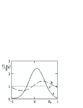
Figure 1: Distribution function $f(p_{x})$ at various values of the driving field and temperature. a — $E=0.1,\;T=0.1$; b — $E=1,\;T=0.1$; c — $E=3,\;T=2$.

The current density (in dimensional units) can be found by a conventional way:

$$j_{x}=\frac{ed}{2\pi\hbar m}\int\limits_{-\pi\hbar/d}^{\pi\hbar/d}p_{x}f(p_{x})\,dp_{x}.$$ (10)

By substitution function (2) into Eq. (10) we get

$$j_{x}=E_{x}+\bigl{[}2\mathrm{erf}\bigl{(}1/\sqrt{2T}\bigr{)}\sinh(1/E_{x})\bigr{]}^{-1}\exp\biggl{(}\frac{T}{2E_{x}^{2}}\biggr{)}$$

$$\times\biggl{[}\mathrm{erf}\biggl{(}\frac{\sqrt{T}}{\sqrt{2}E_{x}}-\frac{1}{\sqrt{2T}}\biggr{)}-\mathrm{erf}\biggl{(}\frac{\sqrt{T}}{\sqrt{2}E_{x}}+\frac{1}{\sqrt{2T}}\biggr{)}\biggr{]}.$$ (11)

Here $j_{x}$ is expressed in units of $j_{0}=ne\Delta d/\pi\hbar$, while all the quantities are written in dimensionless form. Equation (2) determines the current–voltage curve (CVC) for the parabolic miniband 1SL with the current density temperature dependence taking into account. CVC behavior at various temperatures is shown in Fig. 2 (CVC at $T\rightarrow 0$ was shown in Fig. 1 of [6]).

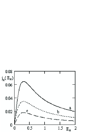
Figure 2: The current density at various temperature values: a - $T=0,5$; b - $T=1$; c - $T=2$.

In limiting case $T\rightarrow 0$ Eq. (2) reduces to the expression found in [6]:

$$j_{x}=E_{x}-\frac{1}{\sinh(1/E_{x})}.$$ (12)

The function (12) reaches maximum at $E_{x}=0.3736818\equiv E_{C0}$. In low fields ($|E_{x}|\ll E_{C0}$) we have

$$j_{x}=\left(1-\sqrt{\frac{2}{\pi T}}\frac{\exp(-1/2T)}{\mathrm{erf}(1/\sqrt{2T})}\right)E_{x}=\left\langle\frac{p_{x}^{2}}{T}\right\rangle_{0}E_{x},$$ (13)

where angle brackets mean averaging over the equilibrium distribution. Note that the mobility temperature dependence in low fields (the expression within round brackets in Eq. (13)) is close to the analogous dependence for the miniband cosine model ($I_{1}(1/2T)/I_{0}(1/2T)$, $I_{n}(z)$ being the modified Bessel function).

Note, that the current maximum $E_{C}(T)$ shifts leftwards (at $E_{x}>0$) and tends to its limiting value $E_{1}=0.2930031$ with rising temperature. Essentially, the $E_{C}$ value does not depend on the temperature at all in the cosine model. Meanwhile, in experiment [8] a shift of $E_{C}$ to lower fields has been found with raising temperature. (In [8] miniband transport in 1SL GaAs/AlAs was investigated in temperature range 10–300 K under fields up to 1.5 kV/cm, and negative differential conductivity was found surely enough.)

We investigated numerically the temperature dependence $E_{C}(T)$. That function can be approximated (with precision in calculations of $10^{-4}$) with the following formula:

$$E_{C}(T)=\sqrt{E_{1}^{2}+(E_{C0}^{2}-E_{1}^{2})\exp(-\beta T)}\quad(E_{x}=\mathrm{const},\;E_{C0}=E(0)),$$ (14)

where $\beta=4.2$. In Fig. 3, the numerical solution ($E_{C}(T)$) of the equation $\partial j_{x}/\partial E_{x}=0$ is shown, the dotted curve being the approximation (14).

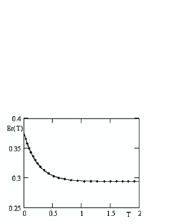
Figure 3: Temperature dependence of the current maximum (Eq. (2)). The dotted line shows approximation (14).

3 Nonequilibrium phase transitions in 2SL

The dispersion law of the square 2SL mentioned in Section 1 takes the form

$$\varepsilon(\mathbf{p})=\varepsilon_{0}+\frac{p_{x}^{2}+p_{y}^{2}}{2m},\quad-\pi\hbar/d<p_{x,\,y}<\pi\hbar/d,$$ (15)

where $\varepsilon_{0}=\mathrm{const}$ is electron energy in the lowest size-quantized level, $\Delta$ is miniband width.

If the coordinate axes are directed along the SL principal ones, then the current density along $X$ axis is given by Eq. (2), while that along $Y$ axis is given by the same formula with $x\rightarrow y$ change.

Now a situation is considered, where the coordinate axes are rotated by angle $45^{\circ}$ with respect the principal axes of the square 2SL. In this case we have

$$j_{y}=E_{y}+\left[4\mathrm{erf}\left(1/\sqrt{2T}\right)\sinh\left(1/(E_{x}+E_{y})\right)\right]^{-1}\exp\left(\frac{T}{2(E_{x}+E_{y})^{2}}\right)$$

$$\times\left[\mathrm{erf}\left(\frac{\sqrt{T}}{\sqrt{2}(E_{x}+E_{y})}-\frac{1}{\sqrt{2T}}\right)-\mathrm{erf}\left(\frac{\sqrt{T}}{\sqrt{2}(E_{x}+E_{y})}+\frac{1}{\sqrt{2T}}\right)\right]$$

$$-\left[4\mathrm{erf}\left(1/\sqrt{2T}\right)\sinh\left(1/(E_{x}-E_{y})\right)\right]^{-1}\exp\left(\frac{T}{2(E_{x}-E_{y})^{2}}\right)$$

$$\times\left[\mathrm{erf}\left(\frac{\sqrt{T}}{\sqrt{2}(E_{x}-E_{y})}-\frac{1}{\sqrt{2T}}\right)-\mathrm{erf}\left(\frac{\sqrt{T}}{\sqrt{2}(E_{x}-E_{y})}+\frac{1}{\sqrt{2T}}\right)\right],$$ (16)

where the field is expressed in units of $\sqrt{2}\pi\hbar/ed\tau$, while the current in units of $\sqrt{2}\pi\hbar/ed\tau$. The formula for $j_{x}$ is obtained from Eq. (3) by interchange $y\leftrightarrow x$.

Let the sample is open in $Y$ direction, so that

$$j_{y}=0.$$ (17)

Then, by substituting Eq. (3) into Eq. (17), we obtain an equation to find the spontaneous transverse field $E_{y}$. At first, consider the case of extremely low temperatures ($T\rightarrow 0$). In that case we get from Eq. (3)

$$j_{y}=E_{y}-\frac{1}{2}\left[\frac{1}{\sinh(1/(E_{x}+E_{y}))}-\frac{1}{\sinh(1/(E_{x}-E_{y}))}\right].$$ (18)

The solution of Eq. (17) in reference to the current (18) has the form

$$E_{ys}=\cases{0,&$0\leq|E_{x}|<E_{C0}$,\cr\pm\sqrt{\frac{\cosh(1/E_{x})}{\sinh^{2}(1/E_{x})}-E_{C0}^{2}},&$|E_{x}|\geq E_{C0}$}.$$ (19)

We write down, for comparison, the analogous formula for the 2SL cosine model:

$$E_{ys}=\cases{0,&$0\leq|E_{x}|<1/\pi$,\cr\pm\sqrt{E_{x}^{2}-1/\pi^{2}},&$|E_{x}|\geq 1/\pi$}.$$ (20)

The numerical solution of Eq. (17) and function (19) (the dotted curve) are shown in Fig. 4.

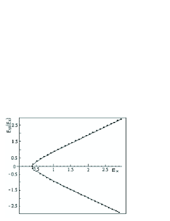
Figure 4: The transverse field $E_{ys}$. The solid line shows numerical solution of Eqs. (17), (18); the dotted one shows function (19).

The solution stability against small enough fluctuations of $E_{y}$ field is determined with the following inequality [9]:

$$\frac{\partial j_{y}}{\partial E_{y}}=\frac{\partial^{2}\Phi}{\partial E_{y}^{2}}>0,$$ (21)

where $\Phi=\int j_{y}dE_{y}+\mathrm{const}$ is a synergetic potential (the entropy production [10]). Conditions (17) and (21) are satisfied at $E_{y}=E_{ys}$. Therefore, the solutions (19) and (20) correspond to minima of the potential $\Phi$, which becomes double-well one (Fig. 5). Thus, there is a NPT2 here.

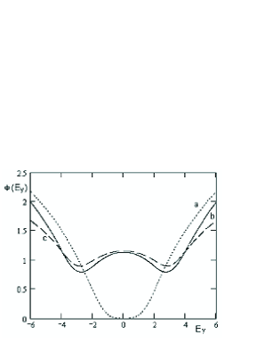
Figure 5: Synergetic potential (up to a constant): a - $E_{x}=E_{C0}$; b - $E_{x}=1$; c - $E_{x}=1$ for the cosine dispersion law.

At $T\neq 0$, the transverse field $E_{y}$ behaves the same way as at $T\rightarrow 0$ with the only difference that the bifurcation point $E_{C}$ shifts leftwards with rising $T$ (for $E_{x}>0$), in complete correspondence with behavior of the current $j_{x}$ maximum (see Fig. (3)).

It follows from the temperature dependence of $E_{C}(T)$, that a novel type NPT2 is possible in the model considered. Indeed, in the field interval $0.317<|E_{x}|<E_{C0}$ the transverse field $E_{ys}(T)$ obeys the following relationship:

$$E_{ys}(T)=\pm\sqrt{\left(E_{C0}^{2}-E_{1}^{2}\right)\left[\exp\left(-\beta T_{C}\right)-\exp\left(-\beta T\right)\right]}\quad(E_{x}=\mathrm{const}),$$ (22)

where the critical temperature is

$$T_{C}=\frac{1}{\beta}\ln\left(\frac{E_{C0}^{2}-E_{1}^{2}}{\cosh(1/E_{x})/\sinh^{2}(1/E_{x})-E_{1}^{2}}\right).$$ (23)

Near the transition point $T_{C}$, the transverse field behaves as $E_{ys}\sim\pm\sqrt{T_{C}-T}$. The NPT2 is illustrated in Fig. 6.

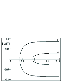
Figure 6: The transverse field $E_{ys}$ at various values of the driving field: a - $E_{x}=0.318$; b - $E_{x}=0.330$.

4 Conclusion

In present paper, an exact distribution function has been found of the carriers in the lowest parabolic miniband of 1SL. The novel formula for the current density in 1SL contains temperature dependence, which leads to the current maximum shift to the low field side with rising temperature, that agrees with available experimental data.

The considered SL model includes NPT’s studied earlier. Besides, a novel type NPT has been found, in which the sample temperature plays a role of a control parameter.

The estimates of the effects predicted are reduced, in general, to estimate of electric field required. At $d=10^{-7}\,\rm{cm}$, $\tau=10^{-12}\,\rm{c}$, we have $E_{0}\approx 2\times 10^{3}\,\rm{V/cm}$. At $E_{x}\approx 600\,\rm{V/cm}$, the value $T_{C}\approx 45\,\rm K$ is obtained.

References

[1]
M. Asche, H. Kostial, O. G. Sarbey, J.Phys. C: Solid State. Phys.13, L645 (1980).
[2]
G. M. Shmelev, E. M. Epshtein, Sov. Phys. - Solid State34,
1375 (1992).
[3]
G. M. Shmelev, E. M. Epshtein, I. A. Chaikovskii, A. S. Matveev, Izv.
AN, ser. fiz.67, 1110 (2003) (in Russian).
[4]
A. S. Matveev, Izv. VGPU (Estestv. i fiz.-mat. nauki), No. 4, 18
(2004) (in Russian).
[5]
G. M. Shmelev, E. M. Epshtein, T. A. Gorshenina, cond-mat/0503092, 2005.
[6]
Yu. A. Romanov, Phys. Solid State45, 559 (2003).
[7]
P. I. Khadzhi, Probability Function, RIO AN MSSR, Kishinev, 1971 (in
Russian).
[8]
H. T. Grahn, K. von Klitzing, K. Ploog, G. H. Döhler, Phys. Rev. B43, 12094 (1991).
[9]
V. L. Bonch-Bruevich, I. P. Zvyagin, A. G. Mironov, Domain Electrical
Instability in Semiconductors, Consultant Bureau, New York, 1975.
[10]
G. M. Shmelev, I. I. Maglevanny, J. Phys.: Condens. Mat.10,
6995 (1998).