A Magnetic Model of the Tetragonal-Orthorhombic Transition in the Cuprates

Abstract

It is shown that a quasi two dimensional (layered) Heisenberg antiferromagnet with fully frustrated interplane couplings (e.g. on a body-centered tetragonal lattice) generically exhibits two thermal phase transitions with lowering temperature – an upper transition at $T_{TO}$ (“order from disorder without order”) in which the lattice point-group symmetry is spontaneously broken, and a lower Néel transition at $T_{N}$ at which spin-rotation symmetry is broken. Although this is the same sequence of transitions observed in La₂CuO₄, in the Heisenberg model (without additional lattice degrees of freedom) $(T_{TO}-T_{N})/T_{N}$ is much smaller than is observed. The model may apply to the bilayer cuprate La₂CaCuO₆, in which the transitions are nearly coincident.

I Introduction

In addressing the physics of high temperature superconductivity (HTC), an important, but often overlooked, issue is the relation between the lattice structure and the electronic physics. In the highly studied “214” family of HTC superconductors, there is a structural phase transition from a high temperature tetragonal (HTT) to a low temperature orthorhombic (LTO) phase with a transition temperature, $T_{TO}(x)$ which drops as a function of doped hole concentration, $x$, from $T_{TO}(0)\approx 500$K in undoped La₂CuO₄, to $T_{TO}(0.22)=0$ in La_2-xSr_xCuO₄ with $x\geq 0.22$ Paul1987 ; Fleming1987 ; Braden1994 ; Gilardi2000 . We were initially motivated to examine the problem of interlayer magnetic coupling because, in the Néel state, the coupling between near-neighbor planes is frustrated in both the T-phase of the 214 compounds (e.g., LSCO and Sr₂CuO₂Cl₂ Greven1994 ), and the T’-phase (e.g. Pr₂CuO₄ or Nd₂CuO₄) Tokura ) due to the location of the Cu²⁺ ions on a body-centered tetragonal lattice. The HTT-LTO transition of the T-phase removes the frustration, and always occurs well above any magnetic ordering temperature, $T_{N}$. On the other hand, no lattice distortion has been identified in the T’ systems, even though the transition temperature to the magnetically ordered Néel state is similar for compounds with the two structures Matsuda1990 ; Keimer1992 .

The question we address is how a purely electronic system, with no lattice coupling, could spontaneously break the point group symmetry which results in the perfect cancellation of the magnetic coupling between the sublattices. This approach is contrary to conventional wisdom, which holds that the HTT-LTO transition in LCO is driven by a lattice parameter mismatch between the CuO₂ planes and the interstitial layer La-O. There are, however, reasons to question whether this explanation is complete: 1) Doping with Ba ions could be expected to relieve the stress more efficiently than doping with Sr, because of its larger ionic radius. It doesn’t seem to do that: the T${}_{TO}\to 0$ at roughly x=0.20 in both cases. 2) The in-plane magnetic susceptibility is found to be spectacularly anisotropic Lavrov2001 ; Lavrov2002 below T_TO ($\chi_{bb}$ is between two and three times larger than $\chi_{aa}$, where $a$ and $b$ refer to the orthorhombic a and b axes); were the electronic anisotropy simply a response to the symmetry breaking lattice distortion, then especially at temperatures above $T_{N}$ but below $T_{TO}$, one would expect the anisotropy of any electronic response to be small in proportion to the magnitude of the orthorhombic distortion, which is around 4% in these materials.

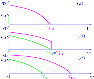
Figure 2: a) The phase diagram for a bilayer system: $T_{N}=0$ $T_{to}\neq 0$. b)The phase diagram for uniform case with $\eta=0$. The transition is first order and $T_{to}=T_{N}$ c) The general phase transition. There are two second order transitions: $T_{to}>T_{N}$.

We consider undoped La₂CuO₄ where, due to the strong repulsions between electrons, the low energy electronic physics is well approximated by a quantum Heisenberg antiferromagnet with a single spin 1/2 on each Cu site. We define a continuum field theory (a $O(N)$ non-linear sigma model with $N=3$) in terms of the corresponding long-wave-length excitations, and solve it in the large $N$ limit (i.e. in the self-consistent phonon approximation). We show that the spin model undergoes a similar sequence of two phase transitions upon cooling as does La₂CuO₄ – a high temperature T-O transition and a lower temperature transition, $T_{N}<T_{TO}$, at which spin-rotation invariance is spontaneously broken resulting in a Neel state. (This corresponds to the schematic phase diagram in Fig. 2c.) The T-O transition in this model is an Ising transition and is an example of “order by disorder without order”, as we explain below. The magnetic order is collinear, consistent with what is determined for La₂CuO₄. However, the difference between the two transition temperatures is very small, $(T_{TO}-T_{N})/T_{N}\ll 1$, while what is observed in La₂CuO₄ is a substantial difference, $(T_{TO}-T_{N})/T_{N}\sim 1$; thus, it is clear that the lattice degrees of freedom play a very significant (possibly dominant) role in the stabilization of the LTO phase in these materials. On the other hand, $T_{TO}$ and $T_{N}$ are very close in the bilayer cuprate La₂CaCuO₆ Ulrich2002 ; Hucker2005 , and the model may apply in this case.

II The microscopic model

We start by defining a model of $M$ coupled layers, each of which consists of a square lattice Heisenberg antiferromagnet, with the sites on one layer situated above the plaquette center of the layer below:

$$H =\sum_{n=1}^{M}\sum_{\vec{R}}\sum_{\vec{\delta}_{0}}\frac{J}{2}\ {\bf S}_{n,\vec{R}}\cdot{\bf S}_{n,\vec{R}+\vec{\delta}_{0}}$$

$$+\sum_{n=1}^{M-1}\sum_{\vec{R}}\sum_{\vec{\delta}_{1}}J_{n}^{\prime}\ {\bf S}_{n,\vec{R}}\cdot{\bf S}_{n+1,\vec{R}+\vec{\delta}_{1}}$$

where ${\bf S}_{n,\vec{R}}$ is the spin at site $\vec{R}$ in plane $n$ and the sums over $\vec{\delta}_{0}$ and $\vec{\delta}_{1}$ run, respectively, over pairs nearest-neighbor sites within a plane and in neighboring planes: $\vec{\delta}_{0}=\pm\hat{x}$, $\pm\hat{y}$ (in units in which the in-plane lattice constant $=1$) and $\vec{\delta}_{1}=\pm(1/2)[\hat{x}+\hat{y}]$, $\pm(1/2)[\hat{x}-\hat{y}]$. Below, we will consider the bilayer ($M=1$) and the body-centered tetragonal ($M\to\infty$) versions of this problem. We will also consider cases in which the spacing between the layers are not all the same so that $J_{n}^{\prime}$ is $n$ dependent, but we will always assume $J\gg J^{\prime}>0$.

In a classically Neel ordered state, ${\bf S}_{n,\vec{R}}={\bf M}_{n}\exp\{i\vec{Q}\cdot\vec{R}\}$ with $\vec{Q}=\langle\pi,\pi\rangle$, there is no coupling between the staggered order parameters, ${\bf M}_{1}$ and ${\bf M}_{2}$, in the two planes. However, high energy short wave-length quantum fluctuations induce an additional effective interaction between the spins at low energy, $H\to H+H_{ind}$:

$$H_{ind}=-\sum_{n=1}^{M-1}\sum_{\vec{R}}K_{n}\left[\Phi_{n,\vec{R}}\right]^{2}$$ (2)

where $\Phi_{n,\vec{R}}\equiv\sum_{\vec{\delta}_{1}}[e^{i\vec{Q}\cdot\vec{\delta}_{1}}{\bf S}_{n,\vec{R}}\cdot{\bf S}_{n+1,\vec{R}+\vec{\delta}_{1}}]$ is a composite order parameter field and $K_{n}\sim(J_{n}^{\prime})^{2}/J$. For $K_{n}>0$, the staggered moments on neighboring planes tend to be colinear to maximize the expectation value of $\Phi$.

Rotation by $\pi/2$ about an axis through any lattice site $\vec{R}$ on plane $n$ is a symmetry of the Hamiltonian. Such a rotation transforms $\phi_{n,\vec{R}}\to-\Phi_{n,\vec{R}}$, so any state with $\langle\Phi\rangle\neq 0$ is a state of broken symmetry. For instance, the state pictured in Fig. 1 has $\langle\Phi_{1,\vec{R}}\rangle<0$, but upon rotation by $\pi/2$ about a site in the lower plane, one obtains the state in which all the spins in the upper layer are reversed, and hence $\langle\Phi_{1,\vec{R}}\rangle$ changes sign. More generally, a non-zero $\langle\Phi_{1,\vec{R}}\rangle$ occurs only in a state in which the discrete C₄ rotational symmetry of the lattice is broken down to C₂, i.e. in an “Ising Nematic” state, or equivalently an electronically orthorhombic state.

III Order from disorder

In two dimensions: A mechanism is called “order by disorder” when it is driven by fluctuation induced terms that are absent at the mean-field level Shender1982 ; Chandra1990 ; Henley1989 . A classic example is the bilayer of Heisenberg antiferromagnet shown in Fig. 1(the case $M=1$). Here, in addition to the usual ground-state degeneracy which is implied by the spontaneous breaking of spin-rotation symmetry, at mean-field level there is an added (continuous) degeneracy due to the frustrated character of the intersystem coupling; the orientation of the staggered magnetization on the upper layer can be rotated by an arbitrary angle relative to that on the lower layer at no cost in energy. However, quantum fluctuations (Eq. 2) lift this degeneracy and produce a preferred relative orientation such that the staggered magnetization on the two planes is colinear. As we have seen, this state also breaks the discrete rotational symmetry of the lattice.

The fluctuations that lead to order by disorder are predominantly short-wavelength, high energy quantum fluctuations, and hence they produce the same tendency for the spins on neighboring planes to be colinear, even when there is no long-range spin order. For instance, since the bilayer problem is a 2D problem, at any finite temperature, $T$, spin rotation symmetry cannot be spontaneously broken. However, the Ising Nematic order can (and does) survive to finite $T$ Cap ; Web ; Biskup2004 . Thus, although originally conceived as being a consequence of small fluctuations about a magnetically ordered state, the tendency of these fluctuations to produce this order persists even when long-wavelength fluctuations have destroyed the antiferromagnetic order, itself, leaving $\xi_{S}(T)<\infty$ -hence Biskup2004 “ordering by disorder without order.”

We can estimate the transition temperature as being the point at which the induced interaction between correlated blocks of spins is of order $T$ (in units in which $k_{B}=1$)

$$K\xi_{S}^{2}\sim T_{TO}^{(bi)}$$ (3)

Since $\xi_{S}\sim\exp[2A\pi J/T]$, the ordering temperature, $T_{TO}^{(bi)}\sim J/\log[J/K]$ is significantly smaller than $J$ only if $K$ is astronomically small. (Here $A\approx 1/4$ for spin 1/2 due to quantum corrections.) The resulting phase diagram is shown in the schematic phase diagram (a) in Fig. 2.

In three dimensions: The magnetic Hamiltonian on the HTT lattice is the three dimensional extension of the same model, where $M\to\infty$ and $J^{\prime}_{n}$ and $K_{n}$ are indenpendent of the layer index, $n$. However, to place the problem in a broader context, in Fig. 2 we have considered a somewhat more general version of this Hamiltonian in which $J\gg J_{2n+1}^{\prime}\equiv J^{\prime}\geq J_{2n}^{\prime}\equiv J^{\prime\prime}>0$ and $K_{n}=K(J_{n}/J^{\prime})^{2}$. For $J^{\prime\prime}/J^{\prime}=1$, this corresponds to the LTT structure of La₂CuO₄, while for $J^{\prime\prime}/J^{\prime}=0$ this corresponds to an array of decoupled bilayers.

The behavior of the phase boundaries for $1\gg J^{\prime\prime}/J^{\prime}>0$ can be readily deduced from the single bilayer results by scaling. The Neel temperature rises steeply from zero as $T_{N}\sim 2A\pi J/\log[J/J^{\prime\prime}]$. The T-O transition rises from its finite bilayer value as $T_{TO}-T_{TO}^{(bi)}\sim J(J^{\prime\prime}/J)^{2/\gamma}$, where $\gamma=7/4$ is the susceptibility exponent of the 2D Ising model.

To obtain a general solution valid for $J^{\prime}\sim J^{\prime\prime}$, we can no longer perturb about the isolated bilayer, and so must rely on other, approximate methods.

IV Continuum O(N) model

We start with the following continuum Hamiltonian,

$$H_{c}=\int\int dxdy\sum_{n=1}^{M}[\frac{1}{2}(\rho_{s}(|\nabla{\bf\phi}_{n}|^{2}+|\nabla{\bf\psi}_{n}|^{2})-g_{1}({\bf\phi}_{n}\cdot{\bf\psi}_{n})^{2}+\frac{\eta_{1}}{2}{\bf\phi}_{n}\partial_{x}\partial_{y}{\bf\psi}_{n}-g_{2}({\bf\phi}_{n}\cdot{\bf\psi}_{n-1})^{2}+\frac{\eta_{2}}{2}{\bf\phi}_{n}\partial_{x}\partial_{y}{\bf\psi}_{n-1}]$$ (4)

where ${\bf\psi}_{n}(\vec{r})$ and ${\bf\phi}_{n}(\vec{r})$ are the local staggered magnetization order parameters in even and odd layers and $|{\bf\phi}_{n}(x,y)|^{2}=|{\bf\psi}_{n}(x,y)|^{2}=1$. Here the spin stiffness $\rho_{s}\propto J$, $g_{1}\propto\frac{J^{\prime 2}}{J}$, $g_{2}\propto\frac{J^{\prime\prime 2}}{J}$, $\eta_{1}\propto J^{\prime}$ and $\eta_{2}\propto J^{\prime\prime}$. (We have considered multiple coupled bilayers, but by making $g$ and $\eta$ dependent on layer index, the more general model can be studied as well.) We also take the order parameters to be $N$ component vectors, generalizing from the physical $N=3$, since in the large $N$ limit (which we expect to be qualitatively correct for $N=3$) the phase diagram of above model can be obtained as follows. The partition function is given by

$$Z=\int D\lambda^{1}D\lambda^{2}D\sigma D\phi D\psi exp(-\int\int dxdy\sum_{n}L_{n})$$ (5)

where the Lagrangian is given by

$$\frac{L_{n}}{N}= \lambda^{1}_{n}(|\vec{\psi}_{n}|^{2}-1)+\lambda^{2}_{n}(|\vec{\phi}_{n}|^{2}-1)+2[\sigma_{1n}(\phi_{n}\cdot\psi_{n})+\sigma_{2n}(\phi_{n}\cdot\psi_{n-1})]+\frac{T\sigma_{1n}^{2}}{g_{1}}+\frac{T\sigma_{2n}^{2}}{g_{2}}+\frac{1}{2T}[\rho_{s}(|\nabla\vec{\phi}_{n}|^{2}+|\nabla\vec{\psi}_{n}|^{2})$$ (6)

$$+\eta_{1}{\bf\phi}_{n}\partial_{x}\partial_{y}{\bf\psi}_{n}+\eta_{2}{\bf\phi}_{n}\partial_{x}\partial_{y}{\bf\psi}_{n-1}]$$

where $\lambda^{i}_{n}(\vec{r}),i=1,2$ are the Lagrangian multiplies for $\vec{\psi}_{n}(\vec{r})$ and $\vec{\phi}_{n}(\vec{r})$ respectively and $\sigma_{in},i=1,2$ are the Hubbard-Stratonovich field. The saddle point of above Lagrangian is determined the following self-consistent equations by taking $\sigma_{in}(r)=\sigma_{i},i=1,2$ and $\lambda_{n}(r)=\lambda$ (subject to the stability condition $2\lambda\geq|\sigma_{1}+\sigma_{2}|$):

$$\sigma_{i} = \frac{-g_{i}}{(2\pi)^{3}}\int d^{2}\vec{k}dk_{z}(cosk_{z}G_{00}-(-1)^{i}sink_{z}G_{01})$$ (7)

$$1 = m^{2}+\frac{T}{(2\pi)^{3}}\int d^{2}\vec{k}dk_{z}G_{00}$$ (8)

where we have taken $\lambda^{i}_{n}(\vec{r})=\lambda,i=1,2$, $m$ is the staggered moment which is non-zero only in the magnetically ordered phase, the integral for $\vec{k}$ has an ultra-violet cuttoff $\Lambda$, and

$$G(k_{x},k_{y},k_{z})=\left(\begin{array}[]{cc}A(\vec{k})&B(\vec{k})\\ -B(\vec{k})&A(\vec{k})\end{array}\right)^{-1},$$ (11)

where $A(\vec{k})=\lambda+\frac{\rho_{s}k^{2}}{k_{B}T}+\frac{cosk_{z}}{2}(\sigma^{+}+\eta^{+}k_{x}k_{y})$ and $B(\vec{k})=i\frac{sink_{z}}{2}(\sigma^{-}+\eta^{-}k_{x}k_{y})$ with $\sigma^{\pm}=\sigma_{1}\pm\sigma_{2}$ and $\eta^{\pm}=\eta_{1}\pm\eta_{2}$ .

First, let us look the uniform case $g_{1}=g_{2}=g,\eta_{1}=\eta_{2}=\eta$ and $\sigma_{1}=\sigma_{2}=\sigma$. If $\eta=0$, the above self consistent equation can be solved exactly. There is a first order transition at $T_{c}$ given by $\frac{g}{4\pi\rho_{s}}=\frac{2\rho_{s}\Lambda}{T_{c}}e^{-4\pi\rho_{s}/T_{c}}$. For $T>T_{c}$, these equations have only one solution: $m=\sigma=0,\lambda=\frac{\rho_{s}\Lambda}{T}e^{-4\pi\rho_{s}/T}$. At $T=T_{c}$ , there is a family of solutions with $m=0$ and $\lambda+\sqrt{\lambda^{2}-\sigma^{2}}=\frac{g}{4\pi\rho_{s}}$. For $T<T_{c}$, the minimal solution has $\sigma=\lambda=g/4\pi\rho_{s}$ and non-zero magnetization,

$$m^{2}=\frac{(T_{c}-T)}{T_{c}}-\frac{T_{c}T}{4\pi\rho_{s}}\log[T/T_{c}].$$ (12)

The transition at $T_{c}$ is a peculiar: The orthorhombic order parameter jumps to a finite expectation value, $\Phi\propto\sigma=g/4\pi\rho_{s}$, just below $T_{c}$, making it a first order transition. At the same time, the magnetization grows continuously from zero as $T$ drops below $T_{c}$. (Unsurprisingly, the coincidence of the two transitions is lifted, as we shall see now, by non-zero $\eta$.) Of course, because $\lambda=\sigma$, there is a gapless (Goldstone) mode for all $T\leq T_{c}$.

When $\eta\neq 0$, there are two phase transitions. The first one is a second order Ising-type transition at $T_{TO}$ and the second one is the Neel transition at $T_{N}$. $T_{TO}>T_{N}$ for any nonzero value of $\eta$. The Ising transition is marked at $T_{TO}$ where $\sigma(T_{TO})=0$ and $\frac{d\sigma}{dT}|_{T=T_{TO}}\neq 0$ and the Neel transition happens at $T_{N}$ where $\lambda=\sigma$. From these conditions, equations which determine $T_{TO}$ and $T_{N}$ can be derived. While it can be proved that the solutions of the equations exist and satisfy $T_{TO}>T_{N}$ when $\eta\neq 0$, it would be tedious to present the proof.

However, when $\eta$ is small, we can solve the critical temperatures up to the second order of $\eta$. Expanding the self consistent equations up to the second order of $\eta$ and defining $\alpha=\frac{g}{4\pi\rho_{s}},\beta=\frac{\eta}{\rho_{s}}$ and $\gamma(T)=\frac{exp(\frac{4\pi\rho_{s}}{T(1+\frac{\beta^{2}}{16})})}{\frac{2\rho_{s}\Lambda}{T}}$, the two critical temperatures are determined by

$$\frac{\gamma(T_{TO})^{-1}}{\alpha}=1+\frac{3\beta^{2}}{16},\frac{\gamma(T_{N})^{-1}}{\alpha}=1+\frac{\beta^{2}}{6}.$$ (13)

From these equations, it is transparent that $T_{TO}>T_{N}$. Up to the second order in $\beta$, the difference between $T_{TO}$ and $T_{N}$ is given by

$$\delta T=T_{TO}-T_{N}=\frac{T_{N}^{2}\beta^{2}}{48(4\pi\rho_{s}-T_{N})}$$ (14)

While this result shows that the fluctuations will induce the Ising order transition before the temperature reaches the Neel transition,

As $\eta$ is expected to be small, it follows that for the uniform case, so is $(T_{TO}-T_{N})/T_{N}$. For nonuniform coupling parameters $g_{1}\neq g_{2}$ and $\eta_{1}\neq\eta_{2}$, there are also two phase transitions and the difference between two transition temperatures can be large. In the large $N$ limit, the Ising transition critical temperature is mainly determined by $g_{1}$ and $\eta_{1}$ while the Neel transition critical temperature is mainly determined by $g_{2}$ and $\eta_{2}$. To show the difference between $T_{TO}$ and $T_{N}$ in this dimerized model, we take $J=0.12ev$, $\eta_{1}/\rho_{s}=0.1$, $\rho_{s}=JS^{2}$, and $g_{i}=0.26JS\Lambda\frac{\eta_{i}^{2}}{\rho_{s}^{2}}$. We choose the cutoff $\Lambda=100$ and $S=1/2$. By varying $\eta_{2}$, we find that the transition temperature $T_{TO}\simeq 470k$, which is almost independent of $\eta_{2}$. In fig.3, we plot $\frac{T_{TO}-T_{N}}{T_{N}}$ as a function of $ln\frac{g_{1}}{g_{2}}$. It fits to a very good linear dependence. So far, there is no experimental evidence supporting layer dimerization along c-axis in cuprates. The quantitative results here can not be directly linked to LCO. However, it will be interesting to see whether the results can be applied in other systems.

If just for a test of the accuracy of the large $N$ method used here, and as a comparison to the result in two dimension, it is interesting to apply the same method to the bilayer problem. The continuum Hamiltonian for this case is $H_{c}$ in Eq. 4 with $M=1$. The corresponding saddle-point equations are obtained from Eqs. 7 by replacing the integral over $k_{z}$ with a sum over $k_{z}=0$, $\pi$. These equations are solved with $m=0$ at all non-zero temperatures. There is, however, a non-zero critical temperature for the T-O transition, $T_{TO}$, such that $\sigma=0$ for $T\geq T_{TO}$, and $\lambda=(\rho_{s}\Lambda/T)\exp[-4\pi A_{\eta}\rho_{s}/T]$ where $A_{\eta}=\sqrt{1-(\eta T/2\rho_{s})^{2}}$. Taking this expression for $\lambda(T)$, the critical temperature is the solution of the implicit equation $4\pi A_{\eta}\rho_{s}\lambda=g$, from which it follows that $T_{TO}\sim 4\pi\rho_{s}/\log[g/\rho_{s}\Lambda]$. As $T$ is decreased below $T_{TO}$, $\sigma$ rises continuously from 0.

V Discussion

In $La_{2-x}Sr_{x}CuO_{4}$, the HTT to LTO transition occurs at roughly twice $T_{N}$, and so is inconsistent with our findings. Probably, this signifies a significant role of the lattice degrees of freedom in driving the transition. However, this does not necessarily imply that the electronic considerations found here are entirely unimportant - in particular, the order one anisotropy in the magnetic susceptibilityLavrov2001 in the temperature range between $T_{N}$ and $T_{TO}$ argues in favor of a significant electronic contribution to the transition. A more compelling case for an electronically driven transition to an orthorhombic phase can be made for the two-layer compound La₂CaCu₂O₆, where the magnetic and structural transitions are observed and they are close together in temperature Ulrich2002 ; Hucker2005 .

It is a very general feature of the fluctuation induced coupling between frustrated planes that $K>0$, and hence that the induced order is collinear. However, a finite concentration of vacancies can induce the opposite sign of interplane coupling which can therefore lead to non-collinear ordering of magnetic moments in different layersHenley1989 . When a vacancy is created in one plane, the LTO order near the vacancy is destroyed. The effect of vacancies on $T_{TO}$ is illustrated in Fig. 4. At mean-field level, the net field applied on any spin in one plane due to the spins in the plane below is zero; however, where there is a vacancy in the lower plane, all the neighboring spins in the next plane feel a net field which is $J^{\prime}$ times minus the spin that was removed to make the vacancy. As is well known, an applied field in an antiferromagnet favors the ordered moments in the plan perpendicular to the field, which permits a net canting of the spins in the direction of the applied field – this is the driving force for the usual spin-flop transition. Thus, there is a negative contribution to the average coupling, $K_{vac}\sim-n_{vac}J^{\prime 2}/J$ which is proportional to the vacancy concentration, $n_{vac}$. We note the AF systems $R_{2}$CuO₄ ($R$= Nd,Pr,Gd,Eu) Sumarlin ; Braden ; Ska ; Chattopadhyay1994 forming in the T’ structure exhibit the combination of no detectable orthorhombic distortion and non-collinear ground states. Possibly, the difference of the T’ compounds from La₂CuO₄ is the moment associated with the rare earth atoms( for Eu atoms, due to the relatively small energy gap between the first excited state and the ground state, they carry significant magnetic moments at 300K although the ground state is nonmagnetic); including them leads to a magnetic Hamiltonian different from Eq. (1).

Acknowledgments: We thank R.J. Birgeneau, M. Greven, B. Keimer, E. Shender, and J. Tranquada for helpful discussions. F. Chen and J.P Hu gratefully acknowledge support by a Purdue research grant. This work was supported in part by the National Science Foundation under grant nos. DMR-0421960 (SAK) and DMR-0520552 (SEB).

Figure 1: A sketch for the bilayer Heisenberg model in square lattice.

Figure 3: The difference between two critical temperatures $\frac{T_{to}-T_{N}}{T_{N}}$ as a function of $ln(g_{1}/g_{2})$.

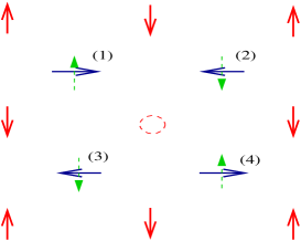
Figure 4: A sketch of spin configurations in presence of one vacancy. When a vacancy is created in one plane, spins in the nearest neighbor plane favor non-collinear alignment. If alignment is collinear, which is illustrated by dashed arrows, the third and fourth spins are not happy energetically.

References

- (1) D. McK. Paul and et al, Phys. Rev. Lett. 58, 1976 (1987)
- (2) R. M . Fleming, et al, Phys. Rev. B 35, 7191 (1987)
- (3) M. Braden, et al, Z. Phys. B 94, 29 (1994)
- (4) R. Gilardi, et al, unpublished.
- (5) M. Greven, et al., Phys. Rev. Lett. 72, 1096 (1994).
- (6) Y. Tokura, H. Takagi, and S. Uchida, Nature, 377, 345 (1988).
- (7) M.Matsuda, et al Phys. Rev. B 42, 10098 (1990).
- (8) B. Keimer, et al., Phys. Rev. B 46, 14034 (1992).
- (9) P. Boni, et al, Phys. Rev. B 38, 185 (1988).
- (10) A. N. Lavrov, et al, Nature 418 , 385 (2002).
- (11) A.N. Lavrov, et al, Phys. Rev. Lett. 87, 017007 (2001)
- (12) C. Ulrich, et al.,Phys. Rev. B 65, 220507 (2002).
- (13) M. Hücker, et al., Phys. Rev. B 71 094510 (2005).
- (14) E.F. Shender, Sov. Phys. JETP 56, 178 (1982).
- (15) C.L. Henley, Phys. Rev. Lett. 62 2056 (1989)
- (16) P. Chandra, P. Coleman and AI Larkin, Phys. Rev. Lett. 64 88 (1990)
- (17) Capriotti L, Fubini A, Roscilde T, et al. Phys. Rev. Lett. 92, 157202 (2004)
- (18) Weber C, Capriotti L, Misguich G, et al. Phys. Rev. Lett. 91, 177202 (2003)
- (19) M. Biskup, et al, Ann. Henri Poincaré 5 1181, (2004)
- (20) T. Chattopadhyay, et al, Phys. Rev. B 49, 9944 (1994)
- (21) M.E. Lines, Phys. Rev, 164, 736 (1967)
- (22) J.B. Parkinson, J. Physics. C, 2, 2012 (1969)
- (23) M. Matsuda, et al, Phys. Rev. B 42, 10098 (1990)
- (24) I. W. Sumarlin, et al, Phys. Rev. B 51, 5824 (1995)
- (25) M. Braden, et al, Europhysics Letters 25, 625 (1994)
- (26) S. Skanthakumar, et al, Phys. Rev. B 47, 6173 (1993)
- (27) T. Chattopadhyay, et al., Phys. Rev. B 49, 9944 (1994).