A lattice of double wells for manipulating pairs of cold atoms

Abstract

We describe the design and implementation of a $2$D optical lattice of double wells suitable for isolating and manipulating an array of individual pairs of atoms in an optical lattice. Atoms in the square lattice can be placed in a double well with any of their four nearest neighbors. The properties of the double well (the barrier height and relative energy offset of the paired sites) can be dynamically controlled. The topology of the lattice is phase stable against phase noise imparted by vibrational noise on mirrors. We demonstrate the dynamic control of the lattice by showing the coherent splitting of atoms from single wells into double wells and observing the resulting double-slit atom diffraction pattern. This lattice can be used to test controlled neutral atom motion among lattice sites and should allow for testing controlled two-qubit gates.

Bose Einstein condensates (BEC) in optical lattices have proven to be an exciting and rich environment for studying many areas of physics, such as condensed matter physics, atomic physics, and quantum information processing (see for instance et al (2005)). Optical lattices are very versatile because they allow dynamic control of many important experimental parameters. Dynamic control of the amplitude of the lattice has been widely used (e.g. et al (2002, 2004, 2002, 2003)); recent experiments have used a state dependent lattice to dynamically control the geometry and transport of atoms in the lattice et al (2003). Recently there have been several proposals for using optical lattices to perform neutral atom quantum computation et al (1999, 1999, 2004). With optical lattices it should be possible to load single atoms into individual lattice sites with high fidelity et al (2004), and then to isolate and manipulate pairs of atoms confined by the lattice in order to perform 2-qubit gates. Loading of single atoms into lattice sites or traps was demonstrated by et al (2002, 2003, 2005, 2005, 2005), but to date no neutral atom based trap can isolate and control interactions between individual pairs of atoms. While previous experiments have demonstrated the clustered entanglement of many atoms confined by an optical lattice et al (2003), the unique ability to isolate and control interactions between pairs of atoms would allow for entanglement between just the pair of atoms.

In this paper we report on a double well optical lattice designed to isolate and control pairs of atoms. The lattice is constructed from two 2D lattices with different spatial periods, resulting in a 2D lattice whose unit cell contains two sites. Within the pair, the barrier height and relative depths of the two sites are controllable. Furthermore, the orientation of the unit cell can be changed, allowing each lattice site to be paired with any one if its four nearest neighbors. The double well lattice is phase stable in that its topology is not sensitive to phase noise from motion of the mirrors. This lattice, in combination with an independent 1D lattice in the third direction to provide 3D confinement, is ideal for testing many 2 qubit ideas, particularly quantum computation based on the concept of “marker atoms” et al (2004) and controlled collisions et al (1999). Among other applications, this lattice could be used for studying tunnel coupled pairs of 1D systems, interesting extensions to the Bose Hubbard model et al (2005), and quantum cellular automata et al (2003).

This paper is divided into six sections. In Section I we discuss the ideal structure of the lattice. Section II describes several experimental issues which need to be considered in order to experimentally realize an ideal double well lattice. Section III details the experimental realization of this lattice and a measurement of the important parameters. In Section IV we show the momentum components present in our lattice by mapping the lattice Bruillion zone. In section V we demonstrate the dynamic control of the properties and topology of the double well lattice by showing the coherent splitting of atoms from a single well into a double well. We summarize and present prospective applications in Section VI.

I Idealized 2D double-well lattice

An ideal double-well lattice would allow for atoms in neighboring pairs of sites to be brought together into the same site, requiring topological control of the lattice structure. It has been shown et al (1993) that a D-dimensional optical lattice created with no more than D+1 independent light beams is topologically stable to arbitrary changes of the relative phases of the D+1 beams. This geometry is usually preferred since phase noise (e.g. that imparted by vibrational noise on mirrors) will merely cause a global translation of the interference pattern. To allow for topological control, a general double-well lattice will necessarily have more than D+1 beams, but it would be desirable to preserve the topological insensitivity due to mirror-induced phase noise. To achieve vibrational phase stability in a D-dimensional lattice made with more than D+1 beams, one can actively stabilize the relative time phase between standing waves et al (2001) et al (1992). Alternatively the lattice can be constructed from a folded, retroreflected standing wave, which forces the relative time phase between standing waves to be a constant  et al (1998). Examples for a 2D case are shown in Fig. 1.

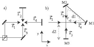
Figure 1: 2D lattices with four beams.(a) Lattices formed by interfering two independent standing waves must be actively stabilized to be topologically phase stable against phase noise caused by vibration of mirrors. (b) Lattices formed from a folded retroreflected beam have intrinsic topological phase stability.

In this paper we consider the latter design, shown in Fig. 1 b. In this scheme, the same laser beam intersects the position of the atom cloud four times. The incoming beam with wave vector $\vec{k}_{1}$ along $\hat{x}$ is reflected by mirrors M1 and M2, and after traveling an effective distance $d_{1}$ (where the effective distance includes possible phase shifts from the mirrors) returns to the cloud with wave vector $\vec{k}_{2}$. The beam is then retroreflected by M3, returning a third time with wave vector $\vec{k}_{3}=-\vec{k}_{2}$, having traveled an additional effective distance $2d_{2}$. Finally, it makes a fourth passage with $\vec{k}_{4}=-\vec{k}_{1}$, traveling again the distance $d_{1}$. The total electric field for this 2D 4-beam lattice is given by Re[$\vec{E}(x,y)e^{i\omega t}$], where

$$\vec{E}(x,y)=E_{1}e^{i\vec{k}_{1}\cdot\vec{r}}\hat{e}_{1}+E_{2}e^{i(\theta+\vec{k}_{2}\cdot\vec{r})}\hat{e}_{2}$$

$$\ \ \ \ +E_{3}e^{i(\vec{k}_{3}\cdot\vec{r}+\theta+2\phi)}\hat{e}_{3}+E_{4}e^{i(2\theta+2\phi+\vec{k}_{4}\cdot\vec{r})}\hat{e}_{4},$$ (1)

and $\vec{r}=x\hat{x}+y\hat{y}$, $\theta=kd_{1}$, $\phi=kd_{2}$, $k=2\pi/\lambda$ ($\lambda$ is the wavelength of the lattice light), and $\hat{e}_{i}$ is the polarization vector of the $i^{th}$ beam. In the absence of polarization rotating elements and ignoring polarization dependent phase shifts from mirrors, $\hat{e}_{4}=\hat{e}_{1}$ and $\hat{e}_{3}=\hat{e}_{2}$. Since the beam retraces the same path, there are only two independent relative phases between the four beams. As a result, the lattice is topologically stable to vibrational motion of M1, M2, and M3; variations in $d_{1}$ and $d_{2}$ result in a simple translation of the interference pattern et al (1998).

The potential seen by an atom in a field Re[${\vec{E}}e^{i\omega t}$] is given by $U=-(1/4)\vec{E}^{*}\cdot\mbox{\boldmath$\alpha$}\cdot\vec{E}$, where $\alpha$ is the atomic polarizability tensor et al (1998). In general, $\alpha$ depends on the internal (angular momentum) state of the atom, having irreducible scalar, vector, and 2^nd rank tensor contributions with magnitudes $\alpha_{s}$, $\alpha_{v}$ and $\alpha_{t}$, respectively. The scalar light shift, $U_{s}=-\alpha_{s}|\vec{E}|^{2}/4$, is state independent and directly proportional to the total intensity. The vector light shift, $U_{v}=i\alpha_{v}(\vec{E}^{*}\times\vec{E})\cdot\hat{F}/4$, depends on the projection of total angular momentum $\hbar\hat{F}$. It can be viewed as arising from an effective magnetic field whose magnitude and direction depend on the local ellipticity of the laser polarization, $\vec{B}_{\rm eff}\sim i\alpha_{v}(\vec{E}^{*}\times\vec{E})$. It vanishes for linearly polarized light. The total vector shift in the presence of a static magnetic field $\vec{B}$ is determined from the energy of an atom in the vector sum field $\vec{B}_{\rm eff}+\vec{B}$. The 2^nd-rank tensor contribution is negligible for ground state alkali atoms far detuned with respect to hyperfine splittings et al (1998), and we will ignore it in this paper.

Consider the ideal situation with four beams of equal intensities ($E_{i}=E$) which intersect orthogonally ($\vec{k}_{1}\cdot\vec{k}_{2}=0$). As a first case consider $\hat{e}_{1}=\hat{y},\hat{e}_{2}=\hat{x}$, where all the light polarizations are in-the-plane. We will refer to this configuration as the “in-plane” lattice. The spatial dependence of the electric field is given by the real part of

$$\vec{E}_{xy}(x,y) = E\left(e^{ikx}+e^{i(2\theta_{xy}+2\phi_{xy}-kx)}\right)\hat{y}$$

$$\ \ \ \ \ +E\left(e^{i(-ky+\theta_{xy})}+e^{i(\theta_{xy}+2\phi_{xy}+ky)}\right)\hat{x},$$

where $\theta_{xy}$ and $\phi_{xy}$ are the path length differences for in-plane light taking into account that the path length difference could be polarization dependent. This gives a normalized total intensity of

$$I_{xy}(x,y)/I_{0} = 2\cos{(2kx-2\theta_{xy}-2\phi_{xy})}$$ (2)

$$\ \ \ \ \ +2\cos{(2ky+2\phi_{xy})+4}$$

where $I_{0}$ is the intensity of a single beam. Due to the orthogonal intersection ($\vec{k}_{1}\cdot\vec{k}_{2}=0$, etc.) and the orthogonality of the polarizations between $\vec{k_{1}}$ and $\vec{k_{2}}$ etc., the resulting four beam lattice is the sum of two independent 1D lattices. As shown in Fig. 2a, this creates a 2D square lattice with anti-nodes (and nodes) spaced by $\lambda$/2 along $\hat{x}$ and along $\hat{y}$. Since the four beam intensities are equal, the lattice forms a perfect standing wave, and the polarization is everywhere linear, although the local axis of linear polarization changes throughout the lattice. In this case the vector light shift vanishes, and the light shift is strictly scalar $U(x,y)=-\alpha_{s}\epsilon_{0}|E(x,y)|^{2}/4$. Note from Eq. 2 that varying $\theta_{xy}$ changes the relative position of the lattice formed by $\vec{k}_{1}$ and $\vec{k}_{4}$, moving the lattice along $\hat{x}$. The phase $\phi_{xy}$ affects both 1D lattices, shifting the combined 2D lattice along $(\hat{x}-\hat{y})/\sqrt{2}$.

As a second case consider ($\hat{e}_{1}=\hat{e}_{2}=\hat{z}$),where all the light polarizations are out-of-the-plane. We will refer to this configuration as the “out-of-plane” lattice. The electric field is given by the real part of

$$\vec{E}_{z}(x,y) = E(e^{ikx}+e^{i(2\theta_{z}+2\phi_{z}-kx)}$$

$$\ \ \ \ \ +e^{i(-ky+\theta_{z})}+e^{i(\theta_{z}+2\phi_{z}+ky)})\hat{z}.$$

where $\theta_{z}$ and $\phi_{z}$ are the path length differences for out-of-plane light. In this case the intensity is not simply a sum of independent functions of x and y, but rather given by

$$I_{z}(x,y)/I_{0} = 4\left[\cos{(kx-\theta_{z}-\phi_{z})}+\cos{(ky+\phi_{z})}\right]^{2}$$ (3)

$$= 16\left[\cos\left(\frac{k}{2}(x+y)-\frac{\theta_{z}}{2}\right)\right]^{2}\$$

$$\ \ \ \ \times\left[\cos\left(\frac{k}{2}(x-y)-\frac{\theta_{z}}{2}-\phi_{z}\right)\right]^{2}.$$

As shown in Fig 2b, the added interference creates components at $k$ in addition to the components at $2k$ resulting in a lattice spacing along $\hat{x}$ and $\hat{y}$ of $\lambda$ rather than $\lambda/2$ (the lattice period along $\hat{x}+\hat{y}$ is $\lambda/\sqrt{2}$). In addition, the nodal structure changes in that there are nodal lines along the diagonals. In particular, every other anti-node of the in-plane lattice is at the intersection of two nodal lines in the out-of-plane lattice. The polarization is everywhere linear along $\hat{z}$, giving rise to a strictly scalar light shift. As with the in-plane lattice, varying $\theta_{z}$ translates the out-of-plane lattice along $\hat{x}$, and varying $\phi_{z}$ translates the lattice along $(\hat{x}-\hat{y})/\sqrt{2}$.

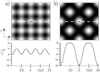
Figure 2: Calculated intensities for in-plane lattice (a) and the out-of-plane lattice (b). Cross sections taken on the white dashed line are shown below their respective plot; a cross is used to denote the origin in each plot. The in-plane lattice has the familiar cos² profile typical of $\lambda/2$ lattices, while the out-of-plane lattice has a cos⁴ profile and periodicity of $\lambda$. The flat portion of the (b) cross section shows the intersection of two nodal lines.

A double well lattice is realized by combining the in-plane and out-of-plane polarizations. Since the polarizations of the two lattices are orthogonal, the total intensity is $I_{tot}=I_{xy}+I_{z}$, and the scalar part of the light shift is simply a sum of the light shifts from the in-plane and out-of-plane lattices. Electro-optic elements in the beam paths $d_{1}$ and $d_{2}$ can produce different phase shifts for different input polarization, allowing for control of the relative phases $\delta\theta=\theta_{z}-\theta_{xy}$ and $\delta\phi=\phi_{z}-\phi_{xy}$, while maintaining vibrational phase stability of the combined lattice. This combined lattice can have a vector light shift, since relative phase shifts between the two polarizations allow for non-zero ellipticity, $i(\vec{E}^{*}\times\vec{E})\neq 0$. If both lattices are everywhere in time-phase ($\delta\theta=0$ or $\pi$ and $\delta\phi=0$ or $\pi$), the vector shift vanishes. Otherwise, there is a non-zero, position dependent $\vec{B}_{\rm eff}(x,y)$ which lies in the $\hat{x}$-$\hat{y}$ plane.

Control of the phase shifts, $\delta\phi$ and $\delta\theta$, and the relative intensity, $I_{xy}/I_{z}$, provides the flexibility to adjust the double-well parameters: the orientation (which wells are paired), the barrier height, and the tilt. For instance, double-well potentials along the $\hat{x}$-direction can be formed by setting $\delta\phi=0$ and $\delta\theta=\pi/2$. Fig. 3 demonstrates how a site can be paired with any one of its four nearest neighbors. Control of the barrier height and of the tilt are shown in Fig. 4.

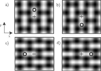
Figure 3: Adjustment of the phases $\delta\theta$ and $\delta\phi$ allow for nearest neighbor pairing with all four nearest neighbors. “+” marks the location of a lattice site located at the origin which can be paired with any of its four nearest neighbors (shown with $\bigcirc$) depending upon the choice of phase: a) $\delta\theta=\pi/2,\delta\phi=-\pi/2$ b) $\delta\theta=-\pi/2,\delta\phi=\pi/2$ c) $\delta\theta=-\pi/2,\delta\phi=0$ d) $\delta\theta=\pi/2,\delta\phi=0$.

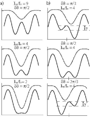
Figure 4: Cross sections of example double well potentials. Solid line represents the double well potential; dotted line shows the placement and amplitude of the out-of-plane lattice. a) The barrier height, labeled above by the quantity $\gamma$, of the double well can be adjusted by placing the out-of-plane lattice “in the barrier” and adjusting the ratio of $I_{xy}/I_{z}$. b) The “tilt” of the double well (the relative offset between adjacent sites) can be changed by adjusting $\delta\theta$ and $\delta\phi$.

II Realistic 2D Double Well Lattice

In the previous section we considered idealized lattices, making assumptions about the amplitudes, wave-vectors and polarizations of the beams in the lattice. In this section we discuss considerations needed to experimentally realize the lattices described above.

II.1 In-plane lattice

For certain applications, such as the realization of the Mott-insulator state et al (2002), we need a nearly perfect in-plane lattice, namely a square 2D lattice with little or no energy offsets between neighboring sites. There are three primary sources of imperfections that affect the performance of the in-plane lattice: imperfect control of the input polarization ($\hat{e_{i}}\cdot\hat{z}=\sin\beta\neq 0$), imperfect alignment causing the beams to be nonorthogonal, ($\vec{k}_{1}\cdot\vec{k}_{2}=\sin\epsilon\neq 0$), and imperfect intensity balance among all four beams ($E_{1}\neq E_{2}\neq E_{3}\neq E_{4}$).

When trying to make a perfect in-plane lattice, if the input polarization is tilted by an angle $\beta$ with respect to the $xy$-plane, then there is a $\hat{z}$ component to the light. The result is a contamination of the in-plane lattice by an out-of-plane lattice that modulates the lattice depth with a periodicity of $\lambda$ (Fig. 5a). Neighboring sites will experience an energy shift $\Delta U=4U_{0}\sin^{2}\left(\beta\right)$ where $U_{0}$ is the depth of a $\beta=0$ in-plane lattice. Since $\Delta U$ scales as $\beta^{2}$ for small $\beta$, the in-plane lattice is fairly tolerant to small rotations of the input polarization. For example, a misalignment of 10 mrad will cause a 0.04% modulation of the trap depth.

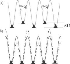
Figure 5: Lattice imperfections causing a) modulation of the lattice depth, $\Delta U$, between neighboring sites and b) state dependent modulation of the barrier height by a polarization lattice. In b) the solid line is the cross section of the intensity lattice; the dashed line is the cross section of the state dependent lattice resulting from unbalanced beam intensities. Atoms in the ground state of each well are shown schematically.

The more stringent demand for minimizing site-to-site offsets of the in-plane lattice is the orthogonality of the two standing waves. If $\vec{k}_{1}\cdot\vec{k}_{2}=\sin\epsilon\neq 0$, standing waves $\vec{k}_{1},\vec{k}_{4}$ and $\vec{k}_{2},\vec{k}_{3}$ have nonorthogonal polarization and give rise to an interference term in the total intensity, thus causing an energy offset between neighboring sites given by $\Delta U\approx 4U_{0}\epsilon$ for small $\epsilon$ (Fig. 5a). This imperfection has the same effect as imperfect input polarization, but is harder to minimize since it scales linearly with $\epsilon$. For example, a misalignment of 10 mrad will cause a 4% modulation of the trap depth. We describe below how to control both imperfections.

The third source of imperfections for the in-plane lattice is the intensity imbalance between the four beams. Experimentally, intensity imbalance can arise from reflection and transmission losses along the beam path as well as from unequal beam waists at the intersection . In general, light imbalance breaks the symmetry between the $x$ and $y$ direction, which removes the degeneracy between the vibrational excitations along $x$ and $y$. Typically, this does not adversely affect the lattice. We also note that since the beam experiences the same losses while traversing $d_{1}$ each time, then for equal beam waists $E_{1}E_{4}=E_{2}E_{3}$, and the losses do not produce well asymmetries.

A more important consequence of intensity imbalance is that the total field is not everywhere linearly polarized, but rather has some ellipticity,

$$\frac{i}{2}(\vec{E}^{*}\times\vec{E})=\left[(E_{1}E_{2}-E_{3}E_{4})\sin(kx+ky-\theta)\right.$$

$$\ \ \ \ \ +\left.\left(E_{1}E_{3}-E_{2}E_{4}\right)\sin(kx-ky-\theta-2\phi)\right]\hat{z}.$$ (4)

This causes a state dependent spatially varying vector light shift with period $\lambda$, even in the absence of the out-of-plane lattice. As evident from Eq. 4, for perfect intensity balance the ellipticity will vanish, resulting in purely linear polarization. Comparing Eq. 2 with Eq. 4 one can see that the phase of the polarization lattice is spatially out of phase with the intensity lattice (see Fig. 5b) resulting in a state dependent barrier height between lattice sites, with relatively little modification of the potential near the minima.

II.2 Out-of-plane lattice

In general, the structure of the out-of-plane lattice is fairly robust against the three imperfections mentioned above. A minor consequence of field imbalance is the possible disappearance of perfect nodal lines. One finds, for example, that at the position of the nodal line intersection, the intensity becomes

$$I_{z,min}=\frac{c\epsilon_{0}}{2}\left(E_{1}-E_{2}-E_{3}+E_{4}\right)^{2}$$ (5)

where $\epsilon_{0}$ is the electric constant (permittivity of free space), and $c$ is the speed of light in vacuum. There are exact nodes when $E_{1}+E_{4}=E_{2}+E_{3}$, and this condition is trivially satisfied when the light fields are balanced. As with the in-plane lattice, degeneracies of vibrational excitations are lifted when the intensities are imbalanced.

II.3 The double-well lattice

A composite in-plane and out-of-plane lattice can be made by adjusting the angle $\beta$ to control the admixture of the two components. For the combined lattice, the consequences and control of imperfections are similar to the in-plane lattice. With the added flexibility to control intensity and relative phase, we can in fact use $\beta$ and $\delta\theta$ to compensate for $\epsilon\neq 0$ (at least for a given magnetic sub-level). The vector light shift for an intensity imbalanced double-well lattice is somewhat more complicated (yet easily calculable), having position dependent ellipticity along $\hat{x}$, $\hat{y}$ and $\hat{z}$. Many experiments are carried out in the presence of a spatially uniform bias field $\vec{B}$, so that the total field seen by the atoms is given by the vector sum $\vec{B}_{\rm tot}=\vec{B}+\vec{B}_{\rm eff}$. For $|\vec{B}|>>|\vec{B}_{\rm eff}|$, the direction of the quantization axis remains nearly constant along $\vec{B}$ throughout the lattice. The magnitude of the state dependent shift in this limit is proportional to

$$|\vec{B}_{\rm tot}| = \sqrt{\left(\vec{B}+\vec{B}_{\rm eff}\right)^{2}}$$ (6)

$$\approx |\vec{B}|+\vec{B}_{\rm eff}\cdot\left(\frac{\vec{B}}{|\vec{B}|}\right),$$

and only the component of $\vec{B}_{\rm eff}$ along $\vec{B}$ contributes to the potential. The ability to adjust the direction of $\vec{B}$ provides significant flexibility in designing state-dependent potentials, and allows for state dependent motion of atoms between the two sites of the double-well.

III Implementation

This double well lattice was implemented on an apparatus described elsewhere et al (2003). ⁸⁷Rb Bose Einstein condensates are produced in an ultra high vacuum glass cell. We use RF evaporation to make BECs with $\approx 200,000$ atoms in the $F=1$, $m_{F}=-1$ hyperfine state. The BEC is confined in a cylindrically symmetric magnetostatic trap with $\omega_{\perp}/2\pi=24$ Hz and $\omega_{\parallel}/2\pi=8$Hz. The Thomas-Fermi radii of condensates are $\approx 15\mu$m and $\approx 40\mu$m respectively, with mean-field atom-atom interaction energy approximately 500 Hz. Atoms in the BEC are then directly loaded into the “tubes” created by the 2D double well lattice potential. The lattice beams are derived from a continuous wave (CW) Ti:Sapphire laser with $\lambda=810$ nm, detuned far from the D1 (795 nm) and D2 (780 nm) transitions in ⁸⁷Rb. On average 2600 in-plane lattice sites or 1300 out-of-plane lattice sites (tubes) are filled with approximately 80 and 160 atoms per site respectively. Due to the tight confinement, the mean-field energy is much larger in the tubes than in the magnetic trap, as much as 7 kHz. During our experiments the magnetic confining potential is left on.

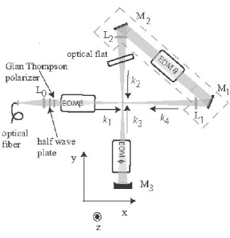
Figure 6: Schematic of the experimental implementation of the 2D double well lattice made from a single folded, retroreflected beam. Mirrors M1 and M2, lenses L1 and L2, and EOM$\theta$ are mounted on a fixed plate.

The experimental schematic of the double well lattice is shown in Fig. 6. An acousto-optical modulator (AOM) provides rapid intensity control of the lattice light. The lattice light is coupled into a polarization maintaining fiber to provide a clean TEM₀₀ spatial mode. A Glan-Thompson polarizer after the fiber creates a well defined polarization in the $xy$-plane. The light is folded by plane mirrors M1 and M2 then retroreflected by concave mirror M3. Lenses L₀, L₁, and L₂, in the input beam and after M1, M2 respectively provide a weak focus (all four beams have 1/e² beam radius of $\approx 170$ $\mu$m) at the intersection of the four beams. A 1 cm thick optical flat after L₂ is used to translate the beam with wave vector $\vec{k}_{2}$ without changing the angle of $\vec{k}_{2}$ relative to $\vec{k}_{1}$. Mirror M3 images the intersection point back onto itself.

Three electro-optic modulators (EOMs): EOM$\beta$, EOM$\theta$, and EOM$\phi$, control the topology of the lattice. EOM$\beta$ is aligned with its fast axis orientated 45^∘ relative to the axis of the Glan-Thompson polarizer, allowing for control of the angle $\beta$, which determines the ratio $I_{xy}/I_{z}=\cot^{2}\beta$. EOM$\theta$ and EOM$\phi$ are aligned with their fast axes in the $xy$-plane allowing for control of the differential phases $\delta\theta$ and $\delta\phi$ respectively. For these initial experiments EOM$\phi$ was not implemented.

L₁, L₂, M1, M2, and EOM$\theta$ are located on a fixed plate. A preliminary alignment of the optics on the fixed plate was performed before installation on the BEC apparatus. In particular, M1 and M2 were first aligned using a penta-prism, and then lenses L₁ and L₂ were inserted and aligned to minimize deflections. The entire plate was mounted next to the BEC apparatus and the input lattice beam, $\vec{k}_{1}$, was aligned to pass through the center of L₁ and L₂. With this technique we measured that we were able to initially align the beams so that the intersection angle deviated from orthogonality by only $\mid\epsilon\mid=$7 mrad.

Calibration of the in-plane lattice depth is achieved by pulsing the lattice and observing the resulting momentum distribution in time-of-flight (TOF) et al (1999). This atomic diffraction pattern reveals the reciprocal lattice of the optical lattice. Diffraction from the perfect in-plane lattice has momentum components at multiples of $\pm 2\hbar k\hat{x}$ and $\pm 2\hbar k\hat{y}$, while diffraction from the out-of-plane lattice has additional components at multiples of $\pm\sqrt{2}\hbar k(\hat{x}\pm\hat{y})$. The diffraction patterns for both lattices after 13 ms TOF are shown in Fig. 7. For 120 mW and at $\lambda=810$ nm, we measure an average lattice depth of $U_{0}=40$E_R (E${}_{R}=\hbar^{2}k^{2}/(2m)=h\times 3.5$ kHz, m is the Rubidium mass) in each of the independent 1D lattices making up the in-plane lattice. As seen in Fig 2b, we calculate that the out-of-plane lattice is four times deeper than the in-plane lattice for equal intensity.

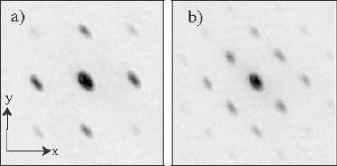
Figure 7: Experimental images of atom diffraction from a 3 $\mu$s pulse of a) the in-plane lattice lattice and b) the out-of-plane lattice after 13 ms time-of-flight.

Pulsing the lattice is a useful method for determining the average in-plane lattice depth, but this method discloses little information about variations in depth $\Delta U$ between adjacent sites of the in-plane lattice (such as variations caused by $\beta\neq 0$ and/or $\epsilon\neq 0$). On the other hand, the ground state wave function of the in-plane lattice is sensitive to $\Delta U$, and we can use this to make $\beta,\epsilon\approx 0$. Information about the ground state can be revealed by adiabatically loading the atoms into the ground band of the lattice et al (2002), quickly switching off the lattice, and observing the atomic momentum distribution in TOF. In this technique the lattice must be turned on slowly enough to avoid vibrational excitation but quickly enough to maintain phase coherence among sites; for our parameters the timescale for loading is $\approx 500$ $\mu$s. (Note that band adiabaticity is more complicated when we combine the in-plane and out-of-plane lattices to create a double well lattice since the tunnel couplings and tilt between double well sites can create situations where band spacings are very small.) For a small but nonzero $\Delta U$, this timescale is not adiabatic with respect to tunneling between neighboring sites. In this way atoms are loaded into every site, even though the true single particle ground state fills every other site. Therefore, atoms are not in an eigenstate of the potential, and the atomic wavefunction evolves in time. In such a lattice potential, pictured in Fig. 5a, atoms in adjacent sites acquire a differential phase, $\Delta Ut/\hbar$. The ground band diffraction pattern changes in time as the atoms are held in the lattice and the differential phase is allowed to “wind up”.

To quantify the “ground band diffraction” patterns, we define a variable $G$ given by

$$G=\frac{N_{1k}-N_{2k}}{N_{1k}+N_{2k}}$$ (7)

where $N_{2k}$ is the number of atoms with momentum components $\pm 2\hbar k\hat{x}$ and $\pm 2\hbar k\hat{y}$, and $N_{1k}$ is the number of atoms with momentum components $\pm\sqrt{2}\hbar k(\hat{x}\pm\hat{y})$ (see Fig. 8a). $G$ is normalized so that the value $G=-1$ corresponds to a diffraction pattern containing only momentum components associated with the in-plane lattice.

We use the ground band diffraction to set the input polarization to $\beta=0$ by observing the dependence of the diffraction pattern on the differential phase shift $\delta\theta$ at a fixed time. For $\beta=0$ the light has no out-of-plane component so that changing $\delta\theta$ with EOM$\theta$ does not change the topology but merely translates the lattice. The calibration of EOM$\beta$ is done by finding the condition in EOM$\beta$ which eliminates the effect of EOM$\theta$, this corresponds to $\beta\approx 0$. In practice for a setting of EOM$\beta$, several ground band diffraction images are analyzed at different values of $\delta\theta$. EOM$\beta$ is then adjusted until scans of $\delta\theta$ produce no noticeable difference in the diffraction pattern.

Sample data for the calibration of $\beta$ is shown in Fig. 8b. This method for determining $\beta=0$ is convenient because it is independent of other lattice imperfections, in particular this method does not rely on $\epsilon=0$. For example the optimal $\beta$ for the data shown in Fig. 8b occurs for $G\approx 0\neq-1$. $G\approx 0$ has no experimental significance; it depends only on the time that the atoms were held in the lattice. A perfect in-plane lattice would have $G=-1$ for all values of $\delta\theta$ at all values of time . The fact that $G\neq-1$ for $\beta=0$ indicates the presence of momentum components at $\pm\sqrt{2}\hbar k(\hat{x}\pm\hat{y})$ due to $\epsilon\neq 0$. With this method we can set $\beta=0$ to zero within 17 mrad, placing an upper limit on $\Delta U/U_{0}\simeq 0.1\%$.

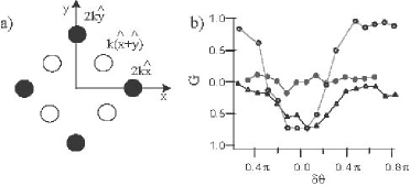
Figure 8: a) Schematic of the momentum components that contribute to $G=(N_{1k}-N_{2k})/(N_{1k}+N_{2k})$. $N_{2k}$ is the sum of atoms in the momentum components designated with filled circles, and $N_{1k}$ is the sum of atoms in momentum comonents designated with open circles. b) Calibration of EOM$\beta$: $\beta\approx$ 52 mrad (open circles), $\beta\approx$ 34 mrad (triangles), and $\beta\approx$ 0 mrad (filled circles).

After setting $\beta=0$ we determine $\epsilon$ by looking at the time dependence of the ground band diffraction pattern. We adiabatically load the lattice in the method described above, then we observe the time oscillations in the ground band diffraction pattern varying between a diffraction pattern with $G=-1$ to $G=+1$. From the time evolution of $G$ (see Fig. 9), we extract the misalignment of the intersection angle, $\epsilon=\Delta U/4U_{0}$. The data (open circles) in Fig. 9 were fit to an exponentially decaying sinusoid (solid line).

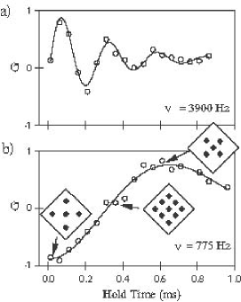
Figure 9: Time dependence of the value $G$ characterizing the diffraction patterns for atoms loaded into lattices with a small offset energy $\Delta U$ caused by $\epsilon\neq 0$. Open circles are data points; solid lines are a fit to the data using a exponentially decaying sinusoid. The frequency of the oscillations given from the fit is inset in each image. From this frequency we determine $\epsilon$: a) $\nu=3900$ Hz corresponds to $\epsilon\simeq 7$ mrad, and b) $\nu=775$ Hz corresponds to $\epsilon\simeq 1.4$ mrad. The data in a) was taken after the initial penta-prism alignment; the data in b) was taken after several iterations of measuring the frequency and then realigning the beams to further improve the angle. Schematics of the diffraction patterns corresponding to different values of $G$ at different times are shown in the insets. The initial phase of G in a) and b) is arbitrary; it depends only on how much phase has been wound up during the loading time.

It is interesting to note the substantial decay in the amplitude of the oscillations in $G$ shown in Fig. 9a, and the reduced rate of decay in Fig. 9b. We do not fully understand this damping, or the reason why the damping is much less for the improved $\epsilon$. Inhomogeneities in the lattice depth due to the Gaussian nature of the lattice beams are not large enough to account for the decay. However, factors such as mean field effects, tunneling, and misalignments between the lattice beams and the magnetostatic trap could contribute to the damping. Regardless of the cause of the decay, we can use this method and the data shown in Fig. 9 to calculate and improve $\epsilon$.

From the fit to the time evolution of G we extract an oscillation frequency, which can be used to calculate $\epsilon$. We calculate $|\epsilon|$ after the initial penta-prism alignment to be 7 mrad $\pm$ 0.2 mrad (Fig. 9a); the energy difference between neighboring sites of a 40 E_r lattice was 3.9 kHz $\pm$ 100 Hz. We reduced $\epsilon$ by adjusting M2 and the optical flat in order to change the angle of $\vec{k}_{2}$ while keeping the beam aligned on the BEC, then remeasured the oscillation frequency of $G$. After several iterations of realignment and measurement, we improved the alignment to $|\epsilon|=$1.4 mrad $\pm$ 0.2 mrad, which corresponds to an energy offset of 775 Hz $\pm$ 70 Hz for a 40 E_r lattice (Fig. 9b). For a 10 E_r lattice the energy offset would be $\lesssim 200$ Hz. It is clear given the signal-to-noise ratio in Fig. 9b that, if required, the angle could be further improved.

We estimate the amount of polarization lattice from the measured intensity imbalance of the four beams. The losses are due to imperfect anti-reflective coatings on optical elements and the uncoated glass cell. The relative depth of the polarization lattice is a function of $\alpha_{v}|\vec{E}^{*}\times\vec{E}|/\left(\alpha_{s}|\vec{E}|^{2}\right)$ . For far-off-resonant traps the ratio $(\alpha_{v}/\alpha_{s})$ becomes small for the $5s_{1/2}$ ground state of ⁸⁷Rb et al (1998, 1997), thus decreasing the polarization lattice depth. From Eq. 6, the size of the vector potential $U_{v}$ depends on the size and orientation of the bias field. For our measured intensities, $I_{2}=0.85I_{1},I_{3}=0.81I_{1}$,and $I_{4}=0.70I_{1}$ with $\lambda=810$ nm, we estimate for the purely in-plane lattice that the maximum ratio $U_{v}/U_{s}$ in the barrier is $\approx 8\%$. In a combined in-plane and out-of-plane lattice, the vector shift can lead to a state dependent tilt. For present experiments the vector shifts are not important, but in future experiments this could be useful to produce state dependent tunnel couplings and state dependent motion.

IV Visualizing the Brillouin Zone

After minimizing the imperfections in the lattices, we can look at the Brillouin zones (BZ) for each of the two lattices. We load atoms into the lattice in 100 ms, a timescale that is slow with respect to both vibrational excitations and atom-atom interaction energies so that atoms homogeneously fill the lowest band. The lattice is then turned off in 500 $\mu$s, mapping the atoms’ quasi-momentum onto free particle momentum states et al (1995, 2002, 2005, 2001, 2005). Atoms that occupied the lowest energy band of a lattice will have momentum contained in the first BZ of that lattice. The mapped zones for both the in-plane and out-of-plane lattice are shown in Fig.  10. As expected the bands are different for the different lattices. This is clear evidence that we have two distinct lattices with distinct momentum components.

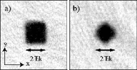
Figure 10: Experimental images after 13 ms TOF of atoms filling the first Brillouin zone for a) the in-plane lattice and b) the out-of-plane lattice. The shapes of the BZs reflect the momentum components in each lattice.

V Dynamic Control of the double well lattice

As an example of the dynamic control of the double well lattice, we demonstrate coherent splitting of atoms from single wells into double wells. Initially, we load into the ground band of the out-of-plane lattice. The time scale for loading (100 ms) is sufficiently slow to ensure dephasing of atoms in neighboring sites. If at this point in time we suddenly turn off the lattice and allow 13 ms TOF, we observe a single, broad momentum distribution, shown in Fig. 11a. Since atoms on separate sites have random relative phases, this distribution is an incoherent sum of “single-slit” diffraction patterns from each of the localized ground state wavefunctions in the out-of-plane lattice. The width of the single-slit pattern is inversely proportional to the Gaussian width of the ground state wave function in each lattice site et al (2003).

To demonstrate the coherent splitting of atoms, we start with the ground-loaded out-of-plane lattice, then dynamically raise the barrier to transfer the atoms into the symmetric double well lattice. The barrier is raised in 200 $\mu$s by increasing the ratio of $I_{xy}/I_{z}$ with EOM$\beta$, while EOM$\theta$ is set to $\delta\theta=\pi/2$ . This timescale is chosen to be slow enough to avoid vibrational excitations but fast enough to maintain phase coherence within a double well. Since there is no phase coherence from one double well to another, the resulting momentum distribution is an incoherent sum of essentially identical double-slit diffraction patterns (shown in Fig. 11b) from each of the wavefunctions localized in individual double wells.

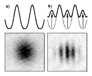
Figure 11: a) Single-slit diffraction pattern resulting from a loss of phase coherence among out-of-plane lattice sites. b) Double-slit interference pattern caused by coherence between atoms within a particular double well but not among the ensemble of double wells.

VI Conclusions

The ability to isolate individual atoms in controllable double well potentials is essential for testing a variety of neutral atom based quantum gate proposals. Two-qubit gate ideas typically involve state dependent motion et al (1999, 1999) or controlled state dependent interaction et al (2004), but nearly all require the ability to move atoms into very near proximity (e.g. into the same site) and subsequently to separate them. The flexibility and dynamic control of the double well lattice can be used to demonstrate and test motion of atoms between wells. Furthermore, state dependence of the barrier height can be used for state dependent motion between wells, allowing for the possibility of 2-atom gates.

In conclusion we have demonstrated a dynamically controllable double-well lattice. The geometry of this lattice is topologically phase stable against vibrational noise, yet allows topological control of the lattice structure. The design of the double well lattice allows for flexible real-time control of its properties: the tilt and the tunnel barrier between sites within the double well. In addition, the orientation of the double well can be adjusted so that a site can be paired with any one of its four nearest neighbors. We have described technical issues and imperfections of the double well lattice, and we have presented techniques to minimize the imperfections. We have demonstrated dynamic control of the double well lattice by showing the coherent transfer of atoms from single wells to double wells. In the future, the double well lattice presented here could be used for applications in quantum computation and quantum information processing, as well as studying interesting extensions of the Bose-Hubbard model, such as the emergence of super-solids and density waves et al (2005).