Structure prediction for cobalt-rich decagonal AlCoNi from pair potentials

Abstract

A systematic, decoration-based technique to discover the atomic structure of a decagonal quasicrystal, given pair potentials and experimentally measured lattice constants, is applied to the “basic” cobalt-rich decagonal Al-Co-Ni quasicrystal. First lattice-gas Monte Carlo simulations are performed, assuming the atomic sites are vertices of a rhombus tiling with edge 2.45Å. This phase is found to be dominated by 13Å diameter decagon-shaped clusters, each with a pentagon of Co atoms at the center. These, and another smaller cluster, decorate vertices of a “binary tiling” with rhombus edge 10.4Å. Further simulations with a restricted site list show that Al arrangements on the borders of the 13Å decagon cluster form Hexagon, Boat, and Star tiles with edge 2.45Å; they indicate specific sites for Co versus Ni atoms, and how the structure adapts to small composition changes. In the second half of the paper, relaxation (augmented by molecular dynamics annealing) is used to obtain realistic structures. The dominant new feature is a set of linear “channels” attractive to Al atoms and running transverse to the layers. Each is typically occupied by three atoms in four layers, implying puckering and a spontaneous period doubling to $c\approx 8$Å. Puckering favors pentagonal long range order of the cluster orientations. Our simulation captures most features of the related $W$-AlCoNi crystal, except for its pentagonal bipyramid motif.

I Introduction

This paper recounts the results of a project to simulate the structure of decagonal quasicrystal Aluminum-Nickel-Cobalt $d$(AlCoNi) in the “basic Co” (cobalt rich) phase purely from energy minimization principles. Of the equilibrium decagonal quasicrystals, $d$(AlCoNi) has (in some of its modifications) the highest structural quality and has received the most study. Studies of the phase diagram indicate that, e.g., decagonal $d$(Al_72.5Co₁₈Ni_9.5) is stable (at higher temperatures only), whereas $d$(AlCo) is metastable only grushko-alco .

Recently, a computational approach was proposed for discovering the atomic structure of any decagonal quasicrystal, given no information except a set of pair potentials, the quasilattice constant, and the periodic lattice constant; it was applied first to $d$(AlCoNi) in the “basic Ni” phase; alnico01 ; alnico02 . In the study described here (and briefly reported elsewhere Gu-letter ; Gu06-ICQ9 ), the same approach is applied to “basic Co” for the first time, and shown to work. As in the “basic Ni” case, our final structure description is in terms of a supertiling with a large quasilattice constant, but here different clusters and tiles enter than in the “basic Ni” case.

Since the sensitivity of the structure to the precise composition is one of the issues in this paper (e.g. in Sec. III.7), and since known structures of crystalline “approximant” phases greatly illuminated our understanding of the related quasicrystals in the past, we shall pause to review what is known in the Al-Co-Ni phase diagram.

The decagonal portion of the Al-Co-Ni phase diagram is fragmented into several modifications occupying small domains. Ri96b ; Ri98 . Of these, those showing the simplest diffraction patterns are the so-called “basic Nickel” phase near the Ni-rich composition Al₇₀Co₁₀Ni₂₀ and so-called “basic Cobalt” near the Co-rich composition Al₇₀Co₂₀Ni₁₀. Several high-resolution X-ray structure determinations were carried out for the “basic Ni” phase xray , but studies of the “basic Co” phase have lagged. An interesting aspect of the Co-rich portion of the phase diagram is the fivefold (rather than tenfold) symmetric decagonal phase, li-5fold . in particular $d$(Al_72.5Co₂₀Ni${}_{7.5})$ and $d$(Al_72.5Co₁₉Ni${}_{8.5})$ ritsch-5fold , also $d$(Al_71.5Co_25.5Ni₃) Ri96a . This and other Co-rich modifications show superstructure diffraction peaks, indicating modulations of the “basic” structure: $d$(Al_72.5Co_17.5Ni₁₀), similar to the “fivefold” modification Ri98 , and $d$(Al₇₁Co₂₀Ni₉), which has a period of 61Å in one direction and thus was called the “one-dimensional quasicrystal” Ri00 . Throughout the phase diagram, the quasilattice constant $a_{0}$ is close to $2.45$Å.

There is a solved periodic crystal approximant of “basic Co”, $W$(AlCoNi) structure Su02 . There are further modifications near to the “basic Ni” composition as well as near $d$(Al₇₀Co₁₅Ni₁₅, and another (partially solved) approximant steurer , with unit cell $37.5$Å $\times 39.5$Å $\times 8$Å, and composition Al₇₁Co_14.5Ni_14.5. The “basic Co” phase has a $4.08$Å stacking period, like “basic Ni”, but it shows much stronger diffuse scattering than “basic Ni”, Fr00a ; Fr00b in such a way as to indicate a local doubling of the $c$ periodicity (to $8.16$Å); the known large approximants also have $c\approx 8$Å. [Later in this paper (Sec. V.1.2), we shall address the stabilizing effects of this period doubling.]

Our general technique is the same as those used in the previous work on “basic Ni”. alnico01 ; alnico02 ; alnico04 . We begin with a small-scale rhombus tiling and discover general motifs and patterns. These patterns usually have a geometry consistent with an inflated Penrose tiling: we define a new model using that tiling, and the patterns observed at the small scale are promoted to be fundamental objects on the inflated tiling. By restricting configurations and increasing the size of fundamental objects, we can run simulations on larger and larger unit cells without excess degrees of freedom, speeding up the MMC process considerably.

The outline of the paper is as follows. After reviewing the technique and the information needed in its set-up (Sec. II), we present initial results in Sec. III from Monte Carlo lattice-gas simulations using a discrete site-list, both with the initial edge-$a_{0}$ rhombi and also with $\tau a_{0}$-edge bilayer rhombi; in particular, the whole structure is built from two cluster modifs – the 13Å decagon  and the Star cluster. Next, Sec. IV codifies this by describing an ideal decoration, which requires specification of the 13Å decagon  orientations as well as the optimum placement of a subset of easily moved Al atoms.

In Sec. V, we pass on to molecular dynamics and relaxation studies that break free of the discrete-site lists; these reveal troughs (which we call “channels”) in the potential energies felt by Al atoms which lead to local disruption of the layering of the atoms, and a breaking of the two-layer peridiocity assumed in previous sections. Here and in Secs. VI and VII, we take up the correlations in the atoms’ displacements, and also how this determines the an ordering of the orientations of 13Å decagon  clusters which reduces the system’s symmetry to pentagonal. We conclude with an application to W(AlCoNi), the best-known approximant of Co-rich quasicrystal $d$(AlCoNi), in Sec. VIII, and a discussion (Sec. IX) of the key results and the limits on their validity.

II Methods and input information

In this section, we lay out the procedures of the simulation, as well as the assumptions and facts that all our results depend on.

II.1 Methods

Our methods are a combination of Metropolis Monte Carlo (MMC), relaxation, and molecular dynamics (MD). We first perform MMC on a set of fixed sites. We create this set by make use of a tiling of Penrose rhombi on each layer and by placing atomic sites on each of the rhombi using a decoration. Fig. 1 shows Penrose rhombi and two decorations that we use. [See Appendix A for a more detailed description of the decoration and tiling.]

Penrose rhombus tilings (even random ones) have a natural inflation rule whereby the same space can be retiled with rhombi whose edges are a power of the golden ratio $\tau\equiv(\sqrt{5}+1)/2\approx 1.618$ multiplied by the orginal edge length. In this paper, we will make use of rhombi with edges $a_{0}=2.45$Å, $\tau a_{0}\approx$3.96Å, and $\tau^{3}a_{0}\approx$10.4Å; we shall also mention a similar tiling with edges $\tau^{2}a_{0}$ that applies to the Ni-rich $d$(AlNiCo) phase, a structure closely related to the one we are investigating.

A unit cell can be tiled in many different ways with the same number of Penrose rhombi; this is physically important since the different tilings correspond to many different configurations of atomic sites that are consistent with the same physical cell and the assumptions based on the lattice constants. To explore this degree of freedom, we perform MMC on the rhombic tiles by using rearrangements of three Penrose rhombi (and the atoms on them) that preserve their collective hexagon outline. The two rhombus configurations for which this is possible are shown in Fig. 1.

Figure 1: These two configurations of Penrose rhombi, with edge $a_{0}\approx 2.46$Å, can be flipped with respect to their asymmetric axes as a way to move sites around.

The MMC is performed on a temperature schedule specified by the beginning and ending inverse temperatures $\beta={{1}/{k_{B}T}}$ along with an inverse temperature step $\Delta\beta$. At each temperature step, a set number of MMC operations per site are performed. After we find a configuration with this “fixed-site” method, we can remove the site list restriction, and use relaxation and MD to find a structure that is more energetically favorable by our potentials.

Why is our method to start with tilings, decorations, and discrete sites, and iterate this (as outlined in the Introduction), rather than immediately perform MD? The reason is that the energy surface of $d$(AlCoNi) in configuration space contains many local energy minima. A pure MD program would be almost certain to be trapped in a glassy configuration. [Even with a small number of atoms and a simpler set of potentials, extremely long MD coolings were necessary in order to produce recognizable (but still quite defective) quasicrystals by brute force. roth97 ]

II.2 Input information

The only experimental inputs into the procedure are lattice constants, composition, and and density; the only theoretical input is the pair potentials. For the initial trials, one must also make a discrete choice of which size of rhombus to use – the quasilattice constant of a decagonal tiling is defined only modulo factors of $\tau$ and one must decide how many atomic layers are to be simulated.

II.2.1 Pair potentials

A-B	$R_{0}^{\rm 0.1eV}$ (Å)	($i$)	$R_{i}$ (Å)	$V_{A-B}(R_{i})$ (eV)
Al-Al	2.62	(0)	2.49	+0.351 (hc)
Al-Co	2.00	(0)	2.30	-0.285 (hc)
		(1)	2.38	-0.302
		(2)	4.44	-0.035
Al-Ni	2.02	(0)	2.25	-0.152 (hc)
		(1)	2.38	-0.192
		(2)	4.37	-0.030
Co-Co	2.48	(0)	2.73	+0.045 (hc)
		(1)	2.68	+0.040
		(2)	4.49	-0.091
		(3)	6.44	-0.033
Co-Ni	2.48	(0)	2.62	+0.050 (hc)
		(1)	2.67	+0.044
		(2)	4.42	-0.081
		(3)	6.39	-0.029
Ni-Ni	2.46	(0)	2.63	+0.051 (hc)
		(1)	2.64	+0.051
		(2)	4.34	-0.075
		(3)	6.30	-0.027

Table 1: Pair potential minima $R_{i}$ for Al-Co-Ni. The “(0)” well is the hard core radius, defined as the minimum radius actually found in a relaxation (after molecular dynamics annealing) of an example configuration; $R_{0}^{\rm 0.1eV}$ is defined by $V_{\rm A-B}(R_{0}^{\rm 0.1eV})=+0.1$eV. Minima are listed only for $|V_{\rm A-B}(R_{i})|>$0.025 eV.

The six pair potentials (for the combinations of Al, Co, and Ni) were generated using Moriarty’s “Generalized Pseudopotential Theory” Mo-GPT , as modified using results from ab initio calculations to add a repulsion correcting the forces between TM-TM nearest neighbors Al-GPT , attributed to many-body terms beyond the pair terms given by GPT. A standard cutoff radius of 7Å was normally used. Even modified, the potentials are imperfect in their unreliable handling of TM-TM nearest neighbors and their neglect of three-body interactions marek-GPT .

The same potentials may be used over the interesting composition range, even though they implicitly depend on electron density, because the lattice constants fortunately compensate so as to keep the electron density nearly constant (over this range). A major post hoc justification for the pair potentials is the correct prediction of binary and ternary phase diagrams widom-GPT-phased . In particular, the (corrected) ternary GPT potentials predict the correct Co-Ni chemical ordering in the approximant $X$(Al₉[Co,Ni]₄) Kat06 and it seems in $W$(AlCoNi) Mi06-ICQ9 .

Radii at which these potentials have minima are given in Table 1, as well as a “hardcore” radius. [Plots of the same potentials are in Fig. 1 of Ref. alnico01, .] As was noted previously Wid96 ; alnico01 the salient features of such potentials are (i) a very strong Al-TM nearest-neighbor well, which is 1.5 times as strong for Al-Co as for Al-Ni; (ii) a rather strong TM-TM second neighbor well [TM-TM first neighbors are unfavorable because they would deprive TM of Al neighbors] (iii) no Al-Al interaction to speak of except the hard core.

A cartoon recipe for an optimum structure is (i) satisfy the TM-TM interactions by a relatively uniform spacing of TM atoms (ii) place as many Al as possible in the Al-TM first wells, limited by the Al-Al hardcore. In principle, the Al-TM optimization might constrain the TM-TM lattice, but in fact the considerable freedom in placing Al’s allows these tasks to be separated. (The main operation of the Al-Al constraints is presumably to select a subset of TM arrangements, which would be practically degenerate if only the TM-TM potentials were taken into account.)

II.2.2 Cell, lattice constant, density and composition

Decagonal quasicrystals are quasiperiodic (at least on average) in just two dimensions. In this decagonal plane, we assume the atomic configuration can be described reasonably well by a tiling of Penrose rhombi with edge length $a_{0}=2.45$Å quasilattice constant, which is experimentally determined. In the dimension normal to the quasiperiodic plane, the $c$-axis, the quasicrystal repeats after a number of two-dimensional quasiperiodic layers are stacked on top of each other with a uniform separation $c/2=2.04$Å taken from experiment.

Periodic boundary conditions are always adopted in all three dimensions: the constraint that this be consistent with a rhombus tiling permits only a discrete family of simulation cells. The cell sizes we chose are especially favorable since they permit a tiling which is close to having five-fold symmetry [in the frequency of the various orientations of rhombi or other objects in the tiling We label our unit cells by their dimensions, $a\times b\times c$, where the stacking period (almost always 4.08Å, and often omitted) comes last (see Table 2). The largest part of our studies were done on the “32 $\times$23” cell, which conveniently has dimensions large enough to accomodate a variety of (dis)ordered arrangements, but small enough to be tractable. We too rarely used the “20$\times$ 38” cell, which has exactly the same area, but a more elongated shape. The 20$\times$ 23 cell has an area smaller by $\tau^{-1}$ than the standard 32 $\times$23; we call it “half-W” as we used it less often than the “W-cell”. That was so called since it has the same dimensions as the approximant $W$-AlCoNi; we employed the “W-cell” even when not trying to predict the $W$-phase structure, for it too has a convenient size. We made the least use of the “20$\times$20 centered”, which is quite small (half the 32$\times$23 cell). For a special purpose we once used the 12$\times$14 cell, which is shorter by a factor $\tau^{-1}$ in each direction than the “half-W” cell; we call it the “Al₁₃Co₄” cell, as it is the same size as the orthorhombic variant of that crystal.

Name	symmetry	a (Å)	b (Å)	$\gamma$
32$\times$23 “standard”	rectangular	32.01	23.25	($90^{\circ}$)
20$\times$20 centered	oblique	19.78	19.78	$72^{\circ}$
20$\times$38 “elongated”	rectangular	19.78	37.62	($90^{\circ}$)
20$\times$23 “half-W”	rectangular	19.78	23.25	($90^{\circ}$)
40$\times$23 “W-cell”	rectangular	39.56	23.25	($90^{\circ}$)
12$\times$14 “Al13Co4”	rectangular	12.22	14.37	($90^{\circ}$)

Table 2: Unit cells used in this work. Note the 20$\times$20 is the primitive cell of the 32$\times$23 centered rectangular lattice, but in an oblique lattice setting so as to give primitive vectors $a$ and $b$ correctly (with angle $\gamma$ between them).

The “basic Co” phase of $d$(AlNiCo) is experimentally known to have a period $c^{\prime}=2c=8.16$Å, but – up till the relaxation studies of Sec. V – we always simulated a cell with a period $c$. In other words, our philosophy (as in Ref. alnico01, ) was to discover as many features as possible in the simplest (4.08Å period) framework, and only later to investigate deviations from this. A partial justification is that an approximate 4.08Å periodicity is expected, and found: many of the atoms do repeat with that period, modulo small offsets. Ideally, though, one should only take the layer spacing from experiment, and investigate cells with different numbers of layers, so as to let the simulation reveal any additional modulations that may increase the period.

Most of our simulations used a standard density FN-bracketdensity of 0.068 atoms/ų and a composition Al₇₀Co₂₀Ni₁₀. Variations of a few percent were tried for special purposes; in particular, our $W$(AlCoNi) simulation (Sec. VIII) used density $\sim$0.071 atoms/ų and composition Al₇₂Co₂₁Ni₇.

In simulations specifically exploring the effect of atom density, we varied it over a range of roughly $0.066$Å^-3 to $0.074$Å^-3 ; this is unphysically loose at one extreme, and unphysically overpacked at the other. A range of roughly $0.066$Å^-3 to $0.072$Å^-3 is internally “legitimate”; our diagnostic for this is that the run-to-run variance of the energy should not be too large. If we took into account competition with other structures in the Al-Ni-Co phase diagram, or if we used the densities appearing in actual approximant phases, presumably the density range would be much smaller. The actual W phase Su02 has a reported density 0.0708Å^-3, or 0.0703Å^-3 when fractional occupancies are best resolved Mi06-ICQ9 . The atomic density in some decagonal approximants is 0.0724 Å^-3 for Al₅Co, 0.0695 Å^-3 for Al₁₃Co₄ (in the mC32 structure variant using the standard nomenclature Pearson ), or 0.0687 Å^-3 for Al₃Ni.

Model	Al (%)	Co (%)	Ni (%)	density (Å-3)
Standard initial	70	20	10	0.068x
$W$(AlCoNi)	71.7	20.8	7.5	0.070x
“basic Ni” ideal	70.0	9.3	20.7	0.0706
idealized W-cell	70.1	22.4	7.5	0.071x

Table 3: Composition and density comparison for various structure models. Experimental densities are surprisingly hard to measure accurately, and composition of the ideal crystal structure is rarely identical to actual compositions of the samples. (Sources: “Basic Ni”, Ref. alnico01, , Sec. III B; $W$-AlCoNi, Ref. Su02, ; Mi06-ICQ9, .)

III Fixed-site simulations

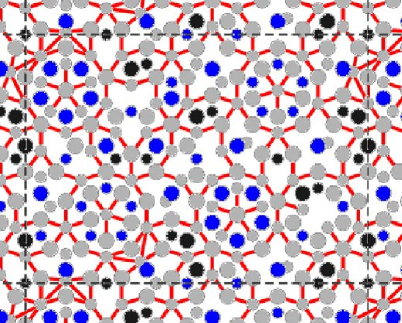
Figure 2: [Color] Typical result of Monte Carlo simulation using 2.45Å edge tiles, on the 32$\times$23 tiling. The composition is Al_0.700Co_0.198Ni_0.101, with 207 atoms in the cell, and the unrelaxed energy is -0.4419 eV/atom. Black circles are Ni, blue are Co, and gray are Al. The [red] lines are a visual aid to mark Al-Al neighbors in different layers, separated by 2.45Å in projection. These mostly form a hexagon-boat-star-decagon tiling as described in Sec. IV. Outer rings of 13Å decagons  can be made out, as well as Star clusters, but have many imperfections, e.g. “short” (2.25Å) Al-Co bonds (see App. B.1.)

In this section, we describe two stages of Metropolis Monte Carlo simulations using discrete site lists, and the key structure motifs that emerged from them. It is important to note that in this kind of run, we are not averaging quantities over the ensemble, nor are we analyzing the final configuration after the lowest-temperature anneal. Instead, we pick out the lowest-energy configuration which has appeared during the entire run. This procedure, since it singles out the low-energy fluctuations, may give meaningful results even when performed at surprisingly high temperatures. FN-highT

III.1 Exploratory simulation using small tiles

A series of annealing simulations and relaxations at the level were performed using the edge $a_{0}$ rhombi. Most of these runs were done on the 32$\times$23$\times$4 unit cell with our standard composition of Al₇₀Co₂₀Ni₁₀ and our standard atomic density of 0.0682 atoms/ų. That unit cell was small enough that it was not computationally prohibitive to simulate, yet large enough that motifs could form without strong constraints by the periodic boundary conditions. FN-cellsize Our aim at this stage is to allow the configurations as much freedom as possible to discover the correct local patterns appropriate to this composition. With the atoms restricted to tile-based sites and the composition and density fixed at our standard values FN-bracketdensity , there still seemed to be sufficient freedom to find good local order, as there had been in the “basic Ni” simulation alnico01 (and in much earlier lattice-gas simulations widom-cockayne ).

To define a Monte Carlo sweep for the 2.45Å edge tiling, we must delve into some technicalities. As we just noted, there are two basic kinds of updates, swaps of atoms between sites and tile-flips. A “sweep” is taken to have one attempted site-swap for each “short bond”, defined as any pair of (candidate) sites separated by less than 3Å. In addition, every sweep contained $\sim 1$ attempted swap per “long bond”, defined to have a separation of 3 – 5 Å. Our standard 2.45Å tile simulation on the 32$\times$23 cell had 680 candidate sites (occupied by about 210 atoms), with about 9.5 short bonds per site and about 67 long bonds per site. Finally , each sweep also had 0.2 attempted tile flips per tile vertex.

A annealing temperature schedule typically began at $\beta=4$ and decreased to $\beta=20$ in increments of $\Delta\beta=1$ or $0.5$, where $\beta$ is measured in (eV)^-1. At each temperature, 100-200 sweeps were performed. The lowest energy encountered during each annealing was saved. (A similar search method was used in Ref. jeong94, .) The annealing cycle was repeated 20 times; the whole set of annealings took about 5 hr on an AMD Athlon 2.1GHz processor. Simulations were run with different temperature schedules, but the results were not noticeably different.

It should be remarked that the lowest temperatures would have been more appropriate for a deterministic decoration forcing a good atomic structure, so that quite small energy differences are being explored. In these exploratory 2.45Å tile simulations, even $\beta=2$ eV^-1 (about three times the melting temperature) can give good structures (keep in mind that the best configuration is saved from each annealing.) Note that the tile-flip degrees of freedom freeze out while the temperature is still high. Which atom configurations are available at lower temperatures depends sensitively on the site-list.

No configuration found by MC annealing (even on the 4Å tiling, see Subsec. III.5) had energy as low as the idealized tiling in Fig. 7. We believe this is an artifact of the very limited sitelist. The TM arrangement freezes at medium temperatures and becomes frozen at low temperatures, as the only MC moves with a small energy difference are Al hops to a vacant site (with – perhaps – Co/Ni swaps at somewhat higher temperatures). A site which is good for a TM is generally not good for Al, and vice versa, so there are no low-energy Al/TM swaps; a rearrangement of more than two atoms is needed to accomplish such a change.

A typical result is shown in Fig. 2; this has total content Al₁₄₅Co₄₁Ni₂₁ corresponding to our standard conditions. The most striking feature was that the TM atoms organized into a well-patterned sublattice, reminiscent (in $z$-projection) to the packing of pentagons, stars, and partial stars which is one of the canonical representations of Penrose’s tiling. penrose-pentagons The TM atoms configured themselves to be $\sim 4.5$Å apart, inviting a speculation that the longer range patterns are enforced by the TM-TM interactions, while the Al atoms flow around like hard spheres and fill in the gaps. Indeed, there were different “freezing temperatures” for the TM-TM quasilattice and the Al-TM interactions: that is, the TM-TM lattice is well established at a temperature much higher than that necessary to rearrange the Al atoms.

Similar TM patterns are seen in all Al-TM decagonals (with many variations having to do with the placement of the two TM species and the larger-scale arrangement of these large pentagons). So as to best highlight this tiling-like network (and other medium-range structural features) to the eye, our graphics processing was automatically set to show a line connecting every pair of TM atoms in different layers and separated by $\tau a_{0}\approx 4.0$Å in-layer.

A striking effect at this stage is how the Al atoms in the two layers organize themselves into a one-layer network (with edge 2.45Å: see Fig.2). The even vertices are all in one layer and odd vertices within the other layer, so this represents a kind of symmetry-breaking and long-range order that has propagated through the entire simulation cell. In fact, we can already recognize the 2.45Å-edge Decagon-Hexagon-Boat-Star (DHBS) tiling, to be elaborated in Sec. IV.2. Along with this order, and probably driving it, the TM atoms also obey this alternation, except they go in the opposite layer to the layer Al would have gone into. Among other things, that produces large numbers of TM-TM pairs in different layers, separated by $\tau(2.45)\equiv 4.0$Å in-plane and hence by 4.5Å, as described in the previous two paragraphs.

III.2 Fundamental cluster motifs

III.2.1 13Å decagon cluster

It became apparent that at the Al₇₀Co₂₀Ni₁₀ composition, our pair potentials favor the creation of many Al₅TM₅ rings surrounded by two more concentric rings with approximate fivefold and screw decagonal symmetry. The object as a whole will be called the “13Å decagon”(13Å D) for its diameter ($2\tau^{2}a_{0}\approx 12.8$Å).

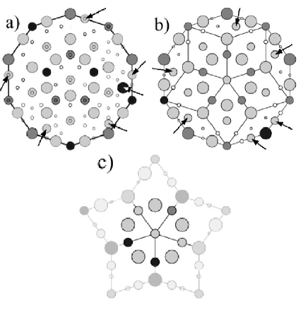
Figure 3: (a)13Å decagon created on the 2.45Å random rhombus tiling at $0.068{\text{\AA{}}}^{-3}$ point density Al₇₀Co₂₀Ni₁₀ composition. Small empty circles denote unoccupied sites. Large and small circles are atoms located in the upper and lower layers, respectively. (Double circles are overlapping circles in two layers.) Black color denotes Ni, dark gray Co, and light gray Al. (b)A 13Å decagon  formed on the 4.0Å tiling and divided into 4.0Å scale Penrose tiles. Here and in (a), arrows point to atom sites (all in ring 2.5 or ring 3) that violate the cluster’s $5m$ symmetry. (c) A Star cluster created on the 4.0Å tiling. Only the darker atoms are considered part of the Star cluster; the lightened atoms belong to adjacent Star clusters or 13Å Ds.

These tiles are decorated by a site list which favors (but does not absolutely force) a 13Å decagon  to appear when Metropolis Monte Carlo is performed. Notice the significantly decreased site list and enchanced ordering, as compared with the version of 13Å D  in (a).

• At the center there is a single Al atom.

• Ring 1 is ten atoms (Al₅TM₅) that we call the ‘5 & 5’ cluster. In projection, they form a decagon, but they alternate in layer, so the symmetry element of the column is ${10_{5}}/m$. The sites in the same layer as the central Al are (almost always) TM sites; the other five sites are normally Al.

• Ring 2 consists of another ten Al atoms; in $z$ projection, each atom is along a ray through an atom of Ring 1 (but in the other layer).

• Ring 3 is on the outer border of the decagon which has edges of length $4.0$Å. In projection, there is a TM atom on each corner alternating in layer (so the actual TM-TM separation is $4.46$Å). These TM atoms sit in the same layer as their Al neighbor in Ring 2. In addition, almost every 13Å decagon edge has an Al atom dividing it in the ratio $\tau^{-1}:\tau^{-2}$, sitting in the opposite layer from the TM atom on the nearer corner. These Al atoms are usually (but not always) closer to the corner TM’s that are in the same layer as the ring 1 TM atoms (see Fig. 3).

• Between rings 2 and 3 are candidate sites which are occupied irregularly by Al, which we will call collectively ring ‘2.5’. [The rules for placement of the ring 2.5 and ring 3 Al will be explored much later (Sec. IV.2).]

At the stage of the $a_{0}=2.45$Å tile simulation, virtually every 13Å D  has imperfections, and there are variations between Co/Ni or Al/vacant in even the best examples; in a typical 13Å D  only 80% of the atoms conform to the above consensus structure, but that is already sufficient to settle what the ideal pattern is.

III.2.2 Star cluster

Filling the spaces between the 13Å decagons, we identify another 11-atom motif similar to the Al₆Co₅ center of the 13Å D: a pentagonal antiprism, in which one layer is all Al atoms, and the other layer is centered by an Al atom. The difference is the five atoms in the second pentagon are only “candidate” TM sites; they have mixed occupation, with roughly 60% TM (usually Ni) and 40% Al. We shall call this small motif the “Star cluster ”, associating it with the star-shaped tile that fills the space in a ring of five adjoining 13Å decagons. (The atoms along the edges, however, are not formally counted as part of the Star cluster: they normally belong either to the outer edge of a 13Å decagon  cluster, or else to another 11-atom Star cluster.)

Such centers were evident in the 2.45Å-edge simulations, but they appear more clearly as repeated patterns in the 4Å-edge simulations. (That tiling must fill the space between 13Å Ds  by 4Å-edge Hexagon, Boat, and Star tiles; the internal vertex of each of those tiles gets a Star cluster  centered on it.)

The local symmetry around the center of a Star cluster  is fivefold (unlike the tenfold local symmetry around the 13Å D). Adjoining Star clusters actually overlap [if we represent them by the star of five rhombi as in Fig. 3(c)] and necessarily have opposite orientations; furthermore, the respective central Al atoms (and surrounding candidate-TM sites) are in alternate layers. Thus, all Star clusters  can be labeled “even” or “odd” according to their orientation.

III.3 Relationships of neighboring decagons

The next step in our general method, after a cluster motif is identified, is to discover what geomeric rules govern the network of cluster centers. Those rules are usually expressed as a list of allowed inter-center vectors, which become the “linkages” Hen91ART of our model geometry. Often, a mild further idealization of this network converts it into random tiling. At that point, one is ready to proceed with the next stage of simulations, based on decorations of this tiling.

So in the present case, once the 13Å decagon  is identified as the basic cluster of our structure, the question is how two neighboring ones should be positioned. (The relative orientations of their pentagonal centers will be left to Sec. VI). As always, the fact that a cluster appears frequently suggests it is favorable energetically, and that one of the geometric rules should be rule to maximize its density. Yet the more closely we place clusters, e.g. overlapping, the more imperfection (deviation from the ideal, fivefold symmetric arrangement) must be tolerated in each cluster; when the clusters are too close, this cost negates the favorable energy. (Note that even if the clusters do not appear to overlap, it is conceivable that a further concentric shell should have been included in the definition of the ideal cluster. In this case, the clusters – properly defined – are still classhing.)

We considered the four candidate linkages in Fig. 4 (a,b,c), but concluded that only the linkages of Fig. 4 (c) were valid. Of course, the frequency by which such patterns appeared spontaneously in our simulations was one clue: edge-sharing is the commonest relationship between 13Å Ds. [Cluster relations like Fig. 4(a,b) did appear on occasion in the 2.45Å-tile simulations, particularly when the simulation cell lattice parameters did not permit a network using only the favorable separations.] Beyond that, we addressed the question more quantitatively by ad-hoc tests in which we arranged that a configuration would (or could) include one of the rarer linkage types, and then compared its energy with a configuration having the common linkages, or checked which of two locations was likelier for another cluster to form. These tests are detailed in Appendix B.

In the Fig. 4(a) linkage, cluster centers are separated $\tau^{3}a_{0}$, and the clusters overlap by a thin Penrose rhombus with edge 4Å. In two places a ring 2 (Al) site of one cluster coincides with a ring 3 (Co) site of the other one, so modifications are mandatory for a couple of atom occupancies. This linkage is motivated by the possibility that the small decagon (bounded by the ring 2 Al atoms) is the key cluster. (Indeed, that decagon, of edge 2.45Å, is one unit of an alternative structural description we shall introduce in Sec. IV.)

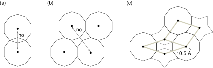
Figure 4: Possible ways for 13Å decagons  to adjoin. (a), (b) Unfavorable ways (c) Actual pattern, forming the “Binary tiling” (edges shown in gray).

Let us forbid overlaps of 13Å decagons  henceforth, and assume that the shortest linkage is edge sharing, a length $1.176\tau^{3}a_{0}\approx 12.2$Å (here $1.176=2\sin 72^{\circ}$) The densest packing of 13Å Ds  would then Hen86 be the vertices of 4Å-edge Hexagons, Boats, and Fat 72^∘ rhombi; that would include many separations by $\sqrt{5}\tau^{2}a_{0}\approx 14.4$Å, like the one across a fat rhombus’s short diagonal as in Fig. 4(b). This linkage also turns out to be disfavorable (Appendix B). The reason appears less obvious than in the overlapping cases, where there were atom conflicts. One viewpoint (adopting the analysis of Sec. IV, below) is that this relationship would not allow the space between 13Å decagon  centers to be filled with 2.45Å  Hexagons, Boats, and Stars. A more direct reason is that at the closest approach, the TM atoms on the respective Decagons’s corners (in different layers) are separated by just $a_{0}$ in layer, or a total distance of 3.19Å, which (see Table 1) is disfavorable.

We are left, then, with a network in which the angles are multiples $(2\pi/10)n$, where $n\geq 3$. We believe that the densest possible packing under these constraints is when the 13Å Ds  sit on the Large sites of a Binary tiling of rhombi with edge $\tau^{2}2.45$Å$\approx 12.2$Å, as in Fig. 4(c). (In this tiling, Large circles sit always on vertices of the short diagonal of the Fat hexagon and of the long diagonal of the Thin hexagon, and Small circles he other way around: this defines an edge matching rule that still allows random-tiling freedom binary .) The second closest possible separation of cluster centers is $1.176\tau^{4}a_{0}$ (the long diagonal of the Thin Penrose rhombus). The Star cluster  clusters go on the Small sites of the Binary tiling.

It should be noted that, in a small or moderate-sized system, the choice of periodic boundary conditions practically determines the network of 13Å decagons  (assuming the number of them is maximized). Consequently, in some unit cells the placement of 13Å D linkages is frustrated, while in others it is satisfied. Those cells mislead us, obviously, regarding the proper linkage geometry; worse, they may mislead us at the prior stage of identifying cluster motifs.

Thus, is conceivable that certain system shapes would favor or disfavor the appearance of 13Å D  clusters, opposite to the infinite-system behavior at the same composition and density. If (as is likely) a significant bit of the cluster stabilization energy is in the linkages, and if there is a competing phase based on other motifs, then the frustration of 13Å D  linkages in a particular cell might tip the balance toward the phase based on the other geometry.

These considerations show why it was important, even in the earliest stages of our exploration, to explore moderately large system sizes (a too small system would not even contain a motif as large as the 13Å D); and also why it must be verified that results are robust against changes in the system shape (i.e. periodic boundary effects). To address this issue, we ran additional simulations on the 20$\times$38$\times$4 cell (Table 2) with the same volume and atom content as our standard 32$\times$23$\times$4 simulation. The lowest energy configurations on this tiling also maximized occurrences of non-overlapping 13Å Ds, although extensive annealing was needed (see App. B.2).

In sections IV and VI, we shall consider decoration rules that divide either the 13Å decagon  network, or the Star cluster  network, into even and odd clusters. It should be recognized that the Binary tilings that fit in the cells in Table 2 are non-generic from this viewpoint. The 13Å D  network has no odd-numbered rings (if it did, that would frustrate any perfectly alternating arrangement of cluster orientations). A corollary is that the Star clusters always appear in (even/odd) pairs: there is never an isolated Star cluster, or any odd grouping.

As detailed in Appendix E, recent structural studies oley06 ; abe06-ICQ9 and simulations Hi06 suggested a cluster geometry based on even larger clusters, with linkages $\tau$ longer than the edges in our tiling. Our initial simulation cells, although much larger than those used previously for the “basic Ni” phase alnico01 , were too small to discover such a cluster. Apart from the possibility of the PB  cluster motif (Sec. VIII.2), the atomic structure of the large cluster models is very similar to ours; in particular, the 20Å cluster is just a 13Å decagon  with two additional rings Consequently the large-cluster model must be quite close in energy to ours (and to a family of similar structures), so it is amazing that a clear pattern (as we found in Appendix E) can ever emerge at the 2.45Å stage, even with annealing. We cannot decide at present which structure is optimal for our potentials.

III.4 Relating structure to potentials

In this subsection, we pause to rationalize the stability of the motifs and structural features identified so far, in terms of the “salient features” of the pair potential interactions (noted in Sec. II.2.1). Notice that, at this stage, no assumptions need be made that atoms in these clusters have stronger energetic binding compared to the other atoms. ICQ9-disc To use clusters as a building block for subsequent structural modeling, it suffices that they are the most frequent large pattern appearing in the structure. (It is convenient if the clusters have a high local symmetry, too.)

We start out explaining some general features . First, the TM (mostly Co) atoms are positioned $\sim$4.5Å apart, right at the minimum of the second (and deepest) well of the potential $V_{\rm Co-Co}(r)$. Second, every Co atom has as many Al neighbors as possible – nine or ten – and as many of those at a distance $R_{1}\approx$2.45Å, close to the particularly strong minimum of $V_{\rm Al-Co}(r)$ (see Table 1). Such coordination shells are, roughly, solutions of the problem of packing as many Al atoms as possible on a sphere of radius $R_{1}$, subject to the constraint of a minimum Al-Al distance (hardcore radius) of $R_{0}=2.6$Å to 2.8Å, which is an fair idealization of the potential $V_{\rm Al-Al}(r)$. Furthermore, since every TM atom is maximizing its coordination by Al atoms, TM-TM neighbor pairs are as rare as possible (and they usually involve Ni, since the Al-Co well is deeper than the Al-Ni well). These features are also true of the “basic Ni” phase and other Al-TM compounds.

Based on an electron channeling technique called ALCHEMI, it was claimed sai00 that for a d(Al₇₂Co₈Ni₂₀) alloy, the Ni and Co atoms are almost randomly mixed on the TM sites. Modeling studies (whether of that Ni-rich composition alnico01 , or the results in this paper for the Co-rich case) suggest that, on the contrary, substantial energies favor specific sites for Ni and Co so the structure is genuinely ternary, not pseudobinary.

To rationalize the $d$-AlCoNi structure in a more detailed way, we must recognize it is locally inhomogeneous in a sense: it is built from two kinds of small motif – small decagons plus Al₉Co clusters – which have quite different composition and bonding. (A third small motif that is neglected by our approach is the $W$-AlCoNi pentagon, a kind of pentagonal bipyramid cluster, which will be discussed in Sec. VIII.) To explain these smaller motifs, we must anticipate part off the descriptive framework of Sec. IV, in which a 2.45Å-edge “HBS” tiling will be introduced.

III.4.1 Small decagon

The heart of the 13Å D  is a smaller decagon (edge $a_{0}=2.45$Å), bounded (in projection) by Al atoms (ring 2). This motif seems to be particularly characteristic of Co-rich structures. Despite the strong tendency to avoid Co-TM pairs, as mentioned just above, this cluster has a ring of five Co neighbors.

Our best explanation is that a conjunction of several Al’s is required in order to compress the Al-Al bonds as short as 2.57Å, but that is advantageous since it allows the Al-Co bonds to be correspondingly shortened to 2.45Å, the bottom of the deep Al-Co potential. The site-energy map (see Fig. 5) shows that the interactions of the ring-1 Co atoms are not very well satisfied, compared to ring-3 Co atoms. On the other hand, the ring-1 Al and (especially) the central Al are well satisfied.

III.4.2 The CoAl₉ coordination shell

This motif consists of a pentagon of five Al atoms centered by Co in one layer, capped by two more Al atoms in the layer above and two in the layer below, so the Co atom has coordination 9 by Al. (A complete pentagon of this sort is centered in each of the 2.45Å-edge Star tiles visible in Fig. 7.) Actually, this motif is almost always surrounded (in projection) by a larger pentagon of five TM, lined up with the Al pentagon, but we shall not treat these Co as part of the motif. They are (often) centers of neighboring CoAl₉-type clusters, as described in the next paragraph.

Two CoAl₉ motifs might be packed by joining the pentagons with a shared edge (two shared Al), but that would create an energetically unfavorable Co-Co distance ($R_{\rm Co-Co}=3.96$Å). If instead two pentagons shared a corner (one Al at the midpoint of the Co-Co line), then $R_{\rm Co-Co}=4.9$Å which is also disfavored. The only way to achieve a favorable $R_{\rm Co-Co}\approx 4.5$Å is to place the two Co in different layers, with some Al atoms from the pentagon around one Co capping the pentagon around the other Co, and vice versa. That is, more or less, the arrangement found around the perimeter of every 13Å decagon  cluster: Finally, if CoAl₉ motifs on the perimeters of two 13Å Ds  are shared, it corresponds to an edge-sharing linkage, and the centers will be $12.2$Å apart, consistent withthe 10.4Å-edge Binary tiling (Subsec. III.4).

The CoAl₉ motif was equally important in the “basic Ni” phase alnico01 .

III.4.3 Site energies map

A diagnostic which was useful in prior investigations using pair potentials Mi96b is the “site energy” for site $i$,

$$E_{i}=\frac{1}{2}\sum_{j}V_{ij}(R_{ij})$$ (1)

where $V_{ij}(R)$ is the proper potential for the species occupying sites $i$ and $j$, and $R_{ij}$ is their separation.

It is revealing to plot $E_{i}$ graphically (Fig. 5). The symbols represent each atom’s site energy minus the average (over the cell) of the site energies for that species, which is our crude surrogate for the chemical potential. The energies are strikingly non-uniform between different places in the structure. An extremely good site energy is obtained for the Al atoms in the even Star cluster. The Co atoms on the 13Å D perimeter, as expected, are much more satisfied than those in the interior. The variable Al atoms in the 13Å D  are the least satisfied, also as expected. The overall picture was not very different when this diagnostic is applied to configurations that, after MD and relaxation, developed puckering with the variable Al entering “channels” (see Sec. V)

Figure 5: Site energies for ideal sites in the configuration of Fig. 7. Here black (white) filled symbols indicate a disfavorable (favorable) deviation, compared to the mean for that species. Circles are Al, up-pointing triangles are Co, and down-pointing triangles are Ni.

The configuration shown is taken from the idealized structure model of Sec. IV. There is a strong contrast between good and bad Al sites; (this is reduced but not eliminated by relaxation and molecular dynamics as in Sec. V). Bad energies are often seen in neighborhoods which are somewhat “overpacked” by Al atoms; when MD is performed (Sec. V), Al atoms are observed to run from these sites to other places which are missing Al atoms. (For example, in the 2.45Å-edge DHBS tiling of Sec. IV, three adjacent 2.45Å Boats is overpacked; if two of them are converted to the combination Hexagon + Star, energy could be lowed by puckering as in Sec. V.)

III.5 4Å rhombus simulations

The $a_{0}=2.45$Å-tile simulations are inadequate, to resolve further details of the atomic structure, such as the exact occupation of ring 2.5/3, or the interactions between 13Å Ds, as these are decided by small energy differences that get overwhelmed by the frequent incorrect occupancies at this level. A new simulation is needed using larger tiles and with a site list reduced as guided by the 2.45Å-tile results It might have been appropriate to try an edge $a_{0}$ hexagon-boat-star tiling (as done in Ref. alnico01, ). However, we chose to go directly to an inflated rhombus tiling with edge $\tau a_{0}\approx 4$Å, which is convenient for decomposing the 13Å decagons(as they have the same edge).

The starting point is that space is tiled with large ${\tau}^{3}a_{0}$ edge length rhombi in a binary tiling. binary The Large disk vertices (which have a local ten-fold symmetry) are then the centers of the 13Å D, as argued in Subsec. III.3. On the actual simulation scale ($\tau a_{0}\approx 4.0$Å), each 13Å D is represented by five fat rhombi arranged in a star, with five thin rhombi surrounding them to form a decagon with five-fold symmetric contents. A decagon in the 4.0Å scale rhombus decomposition is shown in Fig. 3(b).

As compared to the $2.45$Å site list, (i) instead of having independent tilings in the two layers, we now have just one; (ii) the alternation in layers between the sites separated by a $2.45$Å edge is now built in; (iii) there are not many places where the site list allows even a possibility of close distances; (iv) a large fraction of the candidate sites get occupied – the only question is which species. Thus, the $4.0$Å site list is partway to being a deterministic rule. It should be emphasized that this 4.0Å decoration is not well defined on an arbitrary rhombus tiling since the inflated (${\tau}^{3}a_{0}$) tiling must follow a binary tiling scheme. The decoratable tilings are a sub-ensemble of the rhombus random tilings.

The rhombi outside the 13Å Ds  are grouped into 4Å-edge Hexagon, Boat, and Star tiles (a Star cluster  is centered on the interior rhombus vertex of each of these tiles). For example, towards the left side of Fig. 4(c), two 4Å Stars are seen with an overlap (shaped like a “bowtie”) that is resolved by converting either one to a Boat. This decoration of the 4Å rhombi produces a slightly different sitelist, depending on which way such overlaps are resolved, but this did not seem to make a difference for the sites which are actually occupied. FN-sitelist We shall occasionally refer to this version of the 4.0 Å rhombus tiling as the “4.0Å DHBS” tiling.

The $\tau a_{0}$ scale tiling and site list can be naturally deflated back to $a_{0}$-edge Penrose tiles, and these in turn can always grouped into a $a_{0}=2.45$Å-edge Decagon-Hexagon-Boat-Star (DHBS) tiling which is used in Sec. IV and later as a basis of description.

This stage of Metropolis simulation uses only atom swaps, tile flips being disallowed (they would almost always be rejected). We enforce a reduced site list, but do not fix any occupation: any atom (or note) may occupy any sit. The initial inverse temperature was typically $\beta=10$ or $\beta=20$, and increments were $\Delta\beta=1$ or $0.5$ in the 4.0Å-tile annealing runs. FN-4Aanneal (Higher temperatures are not needed since in the $4.0$Å simulations, it is very easy for TM atoms to find their ‘ideal’ sites.) The reduced temperature makes the Al occupancy less random than before.

III.5.1 Use of toy Hamiltonian to generate tilings

To generate appropriate tilings of 4.0Å as a basis for these second-stage lattice-gas simulations, we performed pure tile-flip MC simulations using an artificial “tile Hamiltonian” as a trick. The main term in the Hamiltonian was $-N_{\rm star}$: here $N_{\rm star}$ is the count of star-decagons of 4Å rhombi that are bound to “level 0” ($\nu=0$) sites, using the nomenclature of App. A. (The level 0 condition ensures that such decagons cannot overlap, but only share edges.)

In effect, then, we are maximizing the density of non-overlapping 13Å decagons, with the constraint that the spaces between 13Å Ds  are always tiled with 4Å-edge HBS tiles. Every resulting tiling (even in very large cells) was always a Binary tiling with edge $\tau^{3}a_{0}=10.4$Å as described in Sec. III.3, with a star-decagon on every Large vertex and a star of five fat rhombi on every Small vertex. We conjecture that maximizing the frequency of non-overlapping star-decagons rigorously forces a Binary supertiling; many other examples are known in which maximization of a local pattern leads to a (random) supertiling, decorated with smaller tiles. jeong94 ; Hen98

There is a large ensemble of degenerate ground states of this Hamiltonian, which differ (i) in the Binary tiling network, and (ii) the detailed filling of the 4Å HBS tiles between the star-decagons. Additional terms were used to remove the second kind of degeneracy so that every Binary tiling was still degenerate, but there was a unique (or nearly unique) decomposition of every Binary tiling configuration into 4Å rhombi.

In the Binary tilingsbinary , the Small vertices may occur isolated, but most often form chains. In the “half-W” (or W) unit cell (Fig. 4(d), the chains are unbounded (extending in the $y$ direction), whereas in the 32$\times$23 cell and also the 20$\times$38 cell the chains are just two vertices long.

III.5.2 Results of $4.0$Å edge simulations

The post-hoc justification of the 4.0Å tile decoration is is that its configurations have an energy typically about 0.006 eV/atom lower than a 2.45Å result such as Fig. 2, even though it has a reduced site list. (These lower energy configurations were found in less time and at a lower temperature, too, than on the 2.45Å tiling.) On the $20\times 38$ tiling, the actual low energy configurations found after a 2.45Å-level run of long duration are similar to the those in Fig. 1 of Ref. Gu-letter, , which was created from $4.0$Å simulations.

This suggests to us that this limited ensemble includes all of the lowest-energy states of the original ensemble; the removal of some sites simply keeps the MC from getting stuck in local wells of somewhat higher energy. The most problematic issue of local environments excluded by the site-list reduction was the “short” Al-Co bonds, discussed in Appendix B.1.

We found the 13Å decagon  to be robust, forming in our usual 32$\times$23 cell over a range of compositions Al_0.7Co_0.3-xNi_x for $x=0.05$ to $0.15$ (with the standard density), and also over a range of atom densities 0.066 to 0.076. Å^-3 (at the standard composition Al_0.7Co_0.2Ni_0.1). (These were later checked by simulations with the same atom content on the 4.0Å scale tiling of Subsec. III.5.) In the “$W$(AlCoNi)” unit cell, 13Å Ds  were checked to apppear at densities 0.069 to 0.072 with composition Al_0.718Co_0.211Ni_0.071. Additionally, we confirmed 13Å D  formation when the potentials were cut off at radius 10Å as well as the standard 7Å, or with standard conditions in every unit cell from Table 2.

We can now go beyond the idealized description of idealized clusters, to note some tendencies for variations (especially the TM placement). Although these may be expressed in the language of a rule, they are at this point only statistical biases (primarily based on our 23$\times$32$\times$4 unit cell with our standard composition and density, and mostly using simulations on the 4Å-tiling site list of Sec. III.5.) Only in Sec. IV will these observations be turned into actual rules.

Although we presented rings 2, 2.5, and 3 as having 10-fold symmetry, that is an oversimplification and many site occupations get modulated according to the orientation of the core TM pentagon; (Thus it will not be surprising that a long-range order of the orientations develops, as detailed in Sec. VI.) In particular, the ring 3 Al atoms along the decagon’s edges usually are placed in a layer different from that of the ring 1 TM atoms, which means that (in projection) these Al are alternately displaced clockwise and counterclockwise from the bond center. However, whenever Ni occupies a ring-3 TM site, both the adjacent ring-3 Al atoms tend to adopt the sites in the opposite layer, at a distance of 2.54Å from the Ni, regardless of the core orientation. (Note the adjacent ring-3 TM sites are very likely Co, and this displacement puts the Al-Co distance to 2.45Å, nearly the bottom of the Al-Co well which beats the the Al-Ni attraction.) Finally, if we draw a line from the center of a 13Å D through an Al atom in ring 1 and extend it through the vertex of the 13Å D, the site immediately outside of the decagon along this line (in projection) has a preference for TM with very strong tendencies towards Ni. (If not occupied by Ni or Co, such sites are most often Al rather than vacant.) This induces a relationship between the core orientation and the placement of the Star clusters  that are richer in Ni.

Changes in the net Al density – forced, in our simulations, when we changed the overall density while keeping stoichiometry constant – are accommodated by the 2.5 ring. (The Star cluster  is less flexible: it has a fixed number of atoms.) To anticipate Sec. IV, the ring 2.5/3 Al’s can be alternatively described as the vertices of a Decagon-Hexagon-Boat-Star tiling with edge 2.45Å, and the Al count can be increased by replacing Hexagons and Stars by Boats.

III.6 Effects of TM composition changes

The TM sites in the 13Å decagon(found in ring 1 and ring 3) are normally Co (and otherwise are always Ni) This was checked by a special series of lattice-gas Monte Carlo runs in which only Ni/Co swaps were enabled; this confirmed a Co preference in ring 1. However, when there is an excess of Ni atoms – because either the Ni fraction or the overall density has been increased – Ni atoms start to appear in ring 2.5 of the 13Å D  (in which case the nearby Al atoms behave somewhat differently from their regular patterns). Excess Ni atoms even enter some ring 1 TM sites, in which case the neighboring ring 2.5 (Al) sites are less likely to be occupied (as expected, in light of the powerful Al-Co potential).

When Ni atoms are added at the expense of Co, they typically substitute first for Co(3) on the boundary of a 13Å D, on sites adjacent to Ni of a Star cluster. This presumably disrupts the puckering units that would otherwise be centered on (some of) those Co’s.

We observed how Ni atoms are incorporated without decreasing Co, when the atom density was varied while the same lattice constant and the standard composition Al₇₀Co₂₀Ni₁₀ were maintained. In this case, Ni atoms typically enter ring 2.5 in the 13Å decagon, creating a local pattern of TM occupations that we call the “arrow.” This is convenient to describe in the language of the 4Å rhombus tiling. Say that a 13Å D  corner site is lined up with a Co(1) [ring 1] site and occupied by Ni, and also has am Ni nearest neighbor in an adjacent Star cluster: call these sites Ni(3) and Ni($s$), respectively. Then additional “Ni(2.5)” sites appear inside the 13Å D, in the same layer as the Ni(3). The head of the “arrow” is the 72^∘ angle that Ni($s$) makes with the two Ni(2.5), as in Fig. 6.

The five TM’s [Ni(3) + 2 Ni(2.5) + 2 Co(1)] form a regular pentagon, centered on the Al(2) of the same layer. This Al(2) is also surrounded by Al(1) + 2Al(2) + 2 Al(3) in the other layer, so the combination is an Al₆(TM)₅ just like the core of a 13Å decagon, except that only two of the TM’s are Co, and also the pentagon of five Al’s is quite distorted in this case.

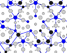
Figure 6: [color] “Arrow” configuration at high Ni density. This pattern is seen at lower right, on the edge of a 13Å decagon in which one Co(1) from the inner ring has been converted to Ni. The overall atom density (0.074 Å^-3) is somewhat above the physical range. At a more realistic density, it appears the same “arrow” configurations and Ni substitutions occur, but much less frequently. The lines in this figure connect pairs of TM atoms in different layers and separated by 4Å in the $xy$ plane. The color conventions for species are the same as Fig. 2.

The density threshold, above which “arrows” appear, was 0.068Å^-3 for the 32$\times$23 tiling, and 0.071Å^-3 for for the W-cell tiling. The difference might be due to our enforcing the standard stoichiometry in both cells, although the ideal Ni:Co ratio must differ since the Star cluster:13Å D  ratio for these cells is, respectively 1:1 and 2:1.

Ni atoms are very often found in Star clusters. When two Star clusters  adjoin, it makes a pair of candidate-TM sites from the respective Star clusters, and these often form a Ni-Ni pair. However, these candidate-TM sites have a large number of Al neighbors, hence one of these is viable site for Co occupation (in which case the other becomes Al). In general, $\sim$2.5Å TM-TM bonds, wherever they are found, will usually be Ni-Ni since this maximizes the number of $\sim$2.5Å Al-Co contacts (recall the Al-Co well is deepest, Al-Ni being only the second deepest well)

III.7 Comparison to Ni-rich decoration

In this subsection, we compare our present results to previous work on the “basic Ni”. phase alnico01 ; alnico02 ; alnico04 .

Our path at this point is actually somewhat different from that taken for the basic Ni structure alnico01 . In the case of “basic Ni”, a hexagon-boat-star (HBS) tiling with a $2.45$Å edge length was used in the analog of our second stage simulations. This was followed by a third stage using an inflated HBS tiling with edges $\tau^{2}a_{0}\approx 6.5$Å (with a deterministic decoration). That description was simple, because (to a good approximation) the decoration was context-independent, i.e. has the same approximate energy independent of which tiles were adjacent. Specifically, all edges were decorated in the same way, and there was no strong constraint relating the Al atoms in the tile interiors to the surrounding tiles. This rule was checked by a simulation at the ideal composition, and the resulting configurations were identical to the ideal decoration, apart from one or two defects per simulation cell.

That template cannot be completely transferred for our Co-rich phase. In this case, it is harder to neglect instances of Co/Ni substitution. In particular, though the TM atoms on the boundary of the decagon object should be idealized as Co, there are special environments in which they clearly are converted to Ni, which introduces a context-dependence into the decoration. Also, there are complicated rules for Al atoms around the outer border of the decagon (i.e. in rings 2.5 and 3), as well as for the occupation of TM atoms in the five candidate sites of the Star cluster. These degrees of freedom interact with the tiling geometry, as well as each other.

Our choice for “basic Co” second stage was to go directly to the 4.0Å DHBS tiling of Sec. III.5 (which is essentially a 10Å edge Binary tiling), thus building in an assumption of the frequency and low energy of the 13Å decagon  cluster. We were not really able to reach a third stage simulation, which properly would have required a complete understanding of puckering and its interactions. Indeed, in Sec. IV we will present a deterministic decoration rule, for a particular composition, taking into account the tendencies noted in Sec. III.5 and Sec. III.6. But this rule is more speculative than the “basic Ni” rule of Ref. alnico01, , in particular no MC simulation reproduced its energy (they were higher, by at least a small energy

III.7.1 Competition of basic-Ni and decagon based structures

We now turn to the physical question of the competition between the Basic-Ni and Basic-Co structure variants in the Al-Co-Ni phase diagram. The “basic Ni” phasse is defined by frequent NiNi nearest-neighbor pairs (forming zigzag chains along the $z$ directions), and Co at centers of a HBS tiling with edge $a_{0}\approx 2.45$Å, without any 5-fold symmetric motif; whereas “basic Co” is defined by the two types of 11-atom pentagonal clusters that form the centers of 13Å decagons  and Star clusters. Now, in Subsec. III.6, it is described how added Ni atoms appear inside the 13Å D  as Ni(2.5), adjacent to Co(3). If we also replace this Co(3)$\to$Ni(3), we get a Ni-Ni pair (TM in a pair always tends to be Ni to free up Co to have more Al neighbors, since Al-Co has a stronger bond than Al-Ni as we have repeatedly remarked.) It is indistinguishable from the characteristic Ni-Ni pair in the “basic Ni” phase of $d$-AlNiCo alnico01 . In other words, the motifs of that phase are appearing continuously as the composition gets richer in Ni. [In the language of the 2.45Å-edge-DHBS small tiling introduced in Sec. IV, the small tile around that TM(3) must become a Hexagon, like the tile in the “basic Ni” decoration alnico01 .]

We incompletely explored this competition by some variations in the site list, in the unit cell size/shape, or in composition. It appears there is a barrier between the basic-Ni and basic-Co structures in our simulations, perhaps a thermodynamic barrier or perhaps merely a kinetic one due to our handling of the degrees of freedom. Thus, there is no assurance that simple brute-force simulation will reach the best state. The only reliable criterion is to anneal each competing phase to a minimum-enegy state, and compare the respective energy values.

’

We used the 12$\times$14 simulation cell for a direct study of the competition of the “basic Ni” and “basic Co” kind of structure; they were found to be practically degenerate in energy throughout the Ni-Co composition range. But in a similar simulation in the standard 32$\times$23 cell, the preference for the Al₆Co₅ rings was much stronger. Our interpretation is that the Al₆Co₅ cluster is not robustly stable by itself, but only when surrounded by the other rings of the 13Å decagon. Since the 12$\times$14 unit cell is too small to allow a proper ring 3, the full benefit of the 13Å D  arrangement is lost and the balance is tilted towards the “basic Ni” type of structure, which is built of smaller (2.45Å-edge HBS) tiles and has no frustration in a cell this size.

It is interesting to note here that the theoretical phase boundary found by Ref. Hi06, in the Al-Co-Ni composition space, running roughly from Al₇₆Co₂₄ to Al₇₀Ni₃₀, corresponds fairly well to the domain Gru04 in which decagonal Al-Co-Ni is thermodynamically stable. In other words, $d$(AlCoNi) occurs at all only when the two competing structure types are close in energy.

A useful diagnostic for the phase competition was used by Hiramatsu and Ishii Hi06 , which might be called the weighted differenced pair distribution function. One takes the difference of the pair distribution function (as a function of radius) between two competing phases, and multiplies it by the pair potentials. The large positive and negative peaks then reveal which potential wells favor which kind of structure. The dominant contributions turned out to be Al-TM nearest-neighbor wells favoring the decagon-based structure, and Al-Al nearest-neighbor repulsion favoring the basic-Ni structure.

III.7.2 20 Å decagons?

We have just observed that using the wrong size of unit cell might spuriously exclude the optimal type of tile or cluster. Thus we may well worry whether even our standard unit cells are large enough to obtain the most correct structure.

Unfortunately, it is not feasible to simulate larger cells using the 2.45Å random-tiling lattice-gas. It would be necessary instead to devise a new decoration, which is more constrained than the 2.45Å sitelist of Sec. III.1 but less constrained than the 4Å rhombus decoration of Sec. III.5. Alternatively, as some conjectured atomic structures are available based on 20 Å decagons (see Appendix E), one might design a decoration which can represent structures built of either 13 Å decagons or 20Å decagons.

The same caveat (about the unit cell size) applies to earlier work by some of us on the “basic Ni” modification.alnico01 In that case, too, electron microscopy studies had suggested structure models having 20Å diameter clusters with pentagonal symmetry abe06-ICQ9 .

IV Idealized decoration

In this section, we present an explicit model structure, derived by idealizing the simulation results of Sec. III, as a decoration of a 10.5Å-edge Binary tiling. Such idealizations are necessarily speculative – they go beyond the simulation observations that inspire them; nevertheless, they are important for several reasons. First, they make available an explicit model for decoration or diffraction. It is trivial to construct a quasiperiodic Binary tiling; decoration of this specifies a quasiperiodic atomic structure, which may be expressed as a cut through a five-dimensional structure, and compared to other models formulated that way. xray ; Yama-AlCoNi-5D ; del06 . (It should not be forgotten that the rules also allow the decoration of random tilings, which among other things can be used to simulate diffuse scattering.)

Second, we hope that a well-defined rule for chemical occupancy corresponds to an energy minimum, in that all the good sites for a particular species are used, and no more. For this reason, it is quite natural that an idealized model has a somewhat different stoichiometry and/or density than the simulations it was abstracted from. Once we have an ideal model, the effect of small density or composition variations may be described by reference to it. The ultimate validation of an idealized model is that it provides a lower energy than any simulations with the same atom content (and lower than other idealized models we may try).

The main issue in passing to a complete rule is to systematize the Al arrangements in rings 2.5 and 3 of the 13Å decagon(which are apparently irregular, and surely not fivefold symmetric), and secondarily the TM arrangements in the Star cluster. This will impel the introduction (Subsec. IV.2 of yet another tiling, the 2.45Å-edge decagon-hexagon-boat-star (DHBS) tiling.

It should be recognized that the details of variable Al around the edge of the 13Å decagon  are crucially modified by relaxation, as will be reported in Secs. V and VII. Nevertheless, we first describe the structure as it emerges within the fixed-site list because (i) this is the path that our method necessarily leads us along; (ii) most of the structure ideas of the fixed-site list have echoes in the more realistic relaxed arrangements. In particular, the ring 2.5 and ring 3 patterns (including short bonds) become the “channels” for Al atoms of Subsec. V.3; the 2.45Å HBS tiles in Subsec. IV and the puckering units of Subsec. VII.2 are centered on the same Co chains; and finally, the fixed-site explanation of the “ferromagnetic” order of 13Å decagon  orientations is closely related to the puckering explanation (Sec. VI).

IV.1 Inputs for the decoration rules

Next we give the starting assumptions (based on Sec. III) which consist of (i) guidelines for the best local environments, given the (fairly artificial) assumption of the fixed-site; (ii) the underlying tile geometry which is to be decorated.

IV.1.1 Guidelines for atom placement

The description inferred from MC runs left undecided (i) the choice of Co versus Ni on sites designated “TM” in the 13Å D; (ii) the choice of Ni, Co, or Al on the sites designated “candidate TM” in the Star cluster; (iii) the location of Al sites in rings 2.5 and 3 of the 13Å D. We seek the minimum energy choices, guided by the salient features of the pair potentials in Table 1 and by the typical configurations resulting from simulations on the 4.0Å tiles (Sec. III.5.2). To resolve details, we also used spot tests (in which selected atoms were flipped by hand) and the site energy function (Sec. III.4.3).

Guideline 1, the strongest one, is the TM-TM superlattice, with separations $\sim 4.5$Å. Note that though Al-TM potentials are stronger than TM-TM, the negligible Al-Al potential seems to allow the TM-TM interaction to dominate the TM placement. This spacing should be enforced particularly for Co-Co, since that potential is somewhat stronger than Co-Ni or Ni-Ni.

Guideline 2 is to maximize number (and optimize the distance) of nearest-neighbor Al-Co contacts, since this potential well is very favorable. A corollary is that TM-TM nearest neighbor pairs tend to be Ni-Co or Ni-Ni (with the glaring exception of five Co in the 13Å D’s core), so as to increase Al-Co at the expense of Al-Ni bonds. (This last fact is more important in a Ni-rich composition alnico01 .)

Guideline 3 is that in the central ring of the Star cluster, the favorable location for Ni (occasionally Co) is on the line joining its center to that of an adjacent 13Å decagon, whenever that line passes over an Al (rather than a TM) atom in ring 1 of the 13Å D. (That line is an edge of a 10.5Å binary tiling rhombus).

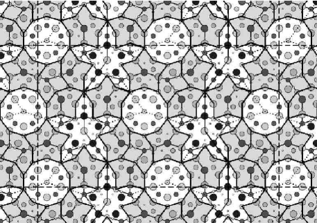
Figure 7: Idealized atom decoration for a bilayer ($c\approx 4$Å) structure on the 40 $\times$ 23 tiling, given an arrangement of 13Å decagons  (shown by light lines). Atom species and layer are identified by same convention as in earlier figures. The 13Å decagon  edges are mostly covered by 2.45Å Stars and Boats, shaded gray, which specify the placement of Al atoms in the Decagon’s ring 2.5 and ring 3. The sites along the lines connecting adjacent Star clusters  are TM (Ni on the even glue cluster and Co on the odd one), as marked by arrows. The even Star clusters  (normally) have Ni in the directions towards the nearest Decagons, as pointed out by dotted lines; these also mark edges of the 10.5Å Binary HBS tiles.

IV.1.2 Binary Hexagon-Boat-Star tiling

Following Subsecs. III.2 and III.3, our decoration is based on a packing of 13Å decagon  clusters and Star clusters  on the 10.5Å-edge binary tiling. We anticipate the results of Sec. VI by orienting the 13Å decagons  all the same way. This has strong implications for the Star clusters. The latter sit on “small” vertices of the Binary tiling, which (as is well known) divide bipartitely into “even” and “odd”sublattices: every 10.5Å  rhombus has one vertex of either kind. Because of the 13Å decagon’s fivefold symmetric core, the adjacent even Star clusters  are not related to it the same as adjacent odd Star clusters. When the 13Å D  cores are all oriented the same, then the Star clusters  of one sublattice – we shall call it Even – have every candidate TM site aligned with ring-1 Al of the adjacent 13Å D  which (by Guideline 3) is favorable for TM occupancy. On the other hand, in the Odd Star clusters  the only sites favorable for TM are the ones adjoining a TM-filled site in the adjacent even Star cluster; the rest of the sites are favorable for Al.

The strong even/odd distinction, and the lack of a prominent pattern on the Odd Star clusters, inspires a slightly different way of representing the 10.5Å tile geometry. If one erases the vertices that center the Odd Star clusters, and the binary-tiling edges that connect to them, the remainding vertices and edges form a hexagon-boat-star tiling with 10.5Å edges. This defines a random tiling model called the “Binary HBS tiling”. (Ref. Mi06-ICQ9, introduced this term, for a different Al-Co-Ni decoration using 4Å-edge tiles, but it has implicitly appeared in some prior decagonal models.) This is not equivalent to the ordinary random HBS tiling, since it is still constrained by additional colorings of the vertices as “large” or “small”, carried over from the Binary tiling. However, it is essentially equivalent to the random Binary tiling, since there is a 2-to-1 correspondence between the tile configurations (depending on which sublattice of “small” vertices is designated “even”).

The Binary HBS tiling, like the cluster orientations, has only a fivefold symmetry, implying a pentagonal space group for the quasicrystal.

2.45Å tile	Content			In 10.5Å tiles		Al nbrs.
	Al	Co	Ni	Fat	Skinny	(each TM)
Decagon	10	5	0	0.6	0.2	4+6
Even Star Cluster	10	5	5	0.2	0.4	3+4
Hexagon	3	1	0	0	0	3+6
Boat	5	1	0	3	0	4+6
Star	6	1	0	0	1	5+4

Table 4: Atom content for decoration in Fig. 7. The names are for tile objects in the 2.45Å-edge DHBS tiling. For the counts in column 1, Al on the tile corners are apportioned according to the corner angle. The numbers of each tile object in the 10.5Å-edge Binary tiling rhombi are also given. The last column gives the Al coordination of the TM atom(s), $m+2n$ where $m$ Al neighbors are in the same layer at 2.45Å, and $2n$ Al neighbors are in the adjacent layers at 2.54Å.

IV.2 The 2.45Å Decagon-Hexagon-Boat-Star tiling

Now we introduce yet another tiling. Its edges are $a_{0}=2.45$Å, as in the initial stage single-layer rhombus tiling, but these tiles are 8Å diameter Decagons, as well as Hexagons, Boats, and Stars, so we call this the “DHBS” tiling. (See Fig. 7). The vertices are decorated with Al atoms, in the even (odd) layers for even (odd) vertices. The 8 Å decagon (with edge 2.45Å) is a subset of the 13Å decagon; its perimeter (vertex) atoms are the ring 2 Al from the 13Å decagon. Each even Star cluster  is represented by five 2.45Å Hexagons in a star arrangement; since these Hexagons are decorated differently from the regular kind, this combined unit will be treated as a separate kind of tiling object called “Even Star cluster”. (An Odd Star cluster  center is just a corner where three 2.45Å Boats or Stars meet.) The 8Å decagons and Even Star clusters, which are fixed once a 10.5Å Binary-HBS tiling is specified, are shown in white in Fig. 7.

The remainder of space – that is, the 13Å decagon borders – becomes tiled with 2.45Å Hexagon/Boat/Star tiles (shown shaded in Fig. 7. The external vertices of the HBS tiles represent all Al(2) [ring 2 of the 13Å D], all Al sites in the Star cluster, and all Al(3) [ring 3]. Each HBS tile interior includes one Co on its “internal vertex” (formed when the HBS tile is subdivided into rhombi), and also Al site(s): one per Hexagon, two in each Boat or Star. These last Al sites represent all Al(2.5) in the 13Å D  and all Al on candidate-TM sites of the Star cluster. Thus, the placement of HBS tiles directly determines that of the ring 3 Al, but not of the ring 2.5 Al. The Even Star type hexagon is a special case: its two internal sites are Co-Ni in the decoration of Fig. 7 but in others (see Subsec. IV.5) would be Ni-Ni.

It should be emphasied that the above description is not just a reformulation of the observations in Sec. III but is, in fact, an additional insight into the motifs emerging from the lattice-gas Monte Carlo on the 4.0Å rhombi. The 2.45Å DHBS tiling is not just used to describe the nearly ground-state structures (which are the focus of this section), but also the less optimal configurations that were our typical best snapshot from a Monte Carlo run (at the 4.0Å stage), or the configurations found when density and composition are somewhat changed, such as in Fig. 6. Despite many irregularities, almost the entire space between Decagons  decomposes into HBS tiles. One difference from the description given above is that, in these imperfect configurations, the Even Star cluster  grouping of 2.45Å Hexagons is seen less; also, either Hexagon filling (TM-TM or Al-TM) may occur anywhere.

It will be noticed that all our decorations of the HBS tiles are identical to those in the “basic Ni” structure alnico01 . The important difference is that in “basic Ni”, there were no 8Å Decagons: the HBS tiles filled space by themselves. This suggests that, as Ni content is increased, conceivably the “basic Co” structure evolves smoothly to the “basic Ni” structure by filling less of space by 8Å decagons, and more of it by HBS tiles.

IV.2.1 Optimization among HBS tilings

The next question is to single out the DHBS tilings with the lowest energies. The particular Al configuration depicted in Fig. 7 was obtained by adjusting Al corresponding to different 2.45Å HBS tilings to optimize the energy in this (40$\times$ 23) unit cell. All the tilings being compared had equal numbers of Al-Co first-well bonds, as well as TM atoms in the same positions, so any energy differences must be due to the second well of $V_{\rm Al-TM}$ (which is about 1/9 as strong as the first well, see Table 1). The total energy difference between two of these states is estimated to be of order 10 – 50 meV.

We can interpret the result in the light of Guideline 2 from Subsec. IV.1.1, together with the last column of Table 3. The largest energy term is proportional to the number of Al-TM (especially Al-Co) bonds; with the fixed sites available, the bond distances are either $2.45$Å (in the same layer) or $2.54$Å (interlayer); the Al-Co potential is stronger at the former separation, leading in principle to smaller energy differences even with the same number of Al-Co bonds. Now, Co centering any HBS tile has a good Al coordination (9 or 10), but this is best in the 2.45Å Boat cluster – mainly because that has more Al atoms. Hence, the number of Boats should be maximized, as is the case in Fig. 7. (Recall that tile rearrangements allow us to trade 2 Boats $\leftrightarrow$ Hexagon + Star in an HBS tiling.)

The TM in the 2.45Å Hexagon tile has a smaller number $Z_{\rm Al}$ of Al neighbors. Thus, if Ni concentration is increased at the expense of Co, the Ni atoms will first occupy these TM sites (on account of the strong Al-Co attraction). Also, where TM-TM neighbors are forced, this tends to occur in 2.45Å Hexagon tiles. For example, the “arrow” motif of induced by increased Ni concentrations just consists of three successive 2.45Å Hexagons on the border of the 13Å decagon, each of them having a TM-TM interior occupation (See Fig. 6).

IV.2.2 Pentagonal bipyramid motif?

The comparison of nearest-neighbor Al coordinations missed one important fact: a 2.45Å Star tile is generally part of a larger motif with pentagonal symmetry. Empirically, it is invariably surrounded by a pentagon of TM atoms (at 4.46Å) in the other layer than the central TM. This means that Star tiles are strongly biased to be on the five 13Å decagon  corners that line up radially with a Co(1) (of the core), and not the other five corners. [That Co(1) is needed to complete the outlying TM pentagon.]

In projection, the five TM atoms surrounding the Star, together with the five Al atoms at its outer points, form a decagon of radius 8Å. The other five Al atoms on the Star’s border turn out to lie in “channels”, in the terminology of the following section (see Sec. V.3), which implies that in a relaxed (and more realistic) structure, these atoms displace out of their layer. The 5 Al + 5 TM atoms forming the outlying decagon all sit in the same layer which turns out to become a mirror (non puckering) layer upon relaxation. In the end, the total motif is simply the “pentagonal bipyramid”, a familiar motif in decagonal structures Hen93 ; Wid96 .

IV.2.3 Alternate description using 4Å DHBS tiles

The decoration depicted in Fig. 7 has 5Ni + 5 Co on the internal sites of the Even Star Cluster, which ensures that the 13Å decagons  have purely Co atoms (never Ni) on their outer vertices (ring 3). The 2.45Å Stars and Boats are the most favorable locations for TM (Co). The Ni site in the even Star cluster  is the least favorable of the TM sites in this decoration.

We pause to express the results in the language of the 4Å-edge DHBS tiling. This tiling has been studied in less detail, for it is less handy than the 2.45Å DHBS or the 10.5Å Binary HBS tilings, for the following reasons: (i) different 4Å HBS tilings, in some circumstances, can correspond to the same atomic configuration; (ii) We lose all hope of systematically describing the Al(2.5) atoms. (iii) the Al(3) variability is now represented by arrows along tile edges, the rules for which are unclear. (We might impose Penrose’s matching rules, on the edges in HBS tiles – leaving the 13Å D edge as a “wild card” that matches anything – however that probably disagrees with the energy minimization.)

The 4.0Å HBS tiles are of course combinations of 4Å rhombi. The 13Å D  is a tile object, while the space between 13Å Ds  gets covered by 4Å Stars, Hexagons, or Boats. The tiles – at least, with the decoration of Fig. 7 – have Co on every exterior vertex (in alternate layers). Each 4Å HBS tile contains, centered on its “interior vertex”, one Star cluster. The 4.0Å HBS tiling is shown in Fig. 8 decorating the 10.5Å

It is appropriate here to review what our decoration does in terms of the originally identified 11-atom Star cluster motif, which (roughly speaking) goes with the 4.0Å DHBS tiling. The decoration of Fig. 7 places Ni on all five of the candidate-TM sites of the Even Star clusters; Odd Star clusters  receive two, one, or zero Co according to whether they occur (see Fig. 8 in a Hexagon, Boat, or Star of the 10.5Å Binary HBS tiling; this Co appears next to each neighboring Even Star cluster.

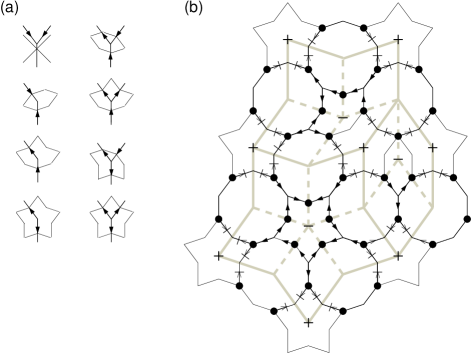
Figure 8: (a). Mapping from an arrow configuration to the 2.45Å-edge HBS tiles in the DHBS tiling. The $\times$ means that two incoming arrows, 72^∘ apart, are never allowed. The arrowed edges belong to the 4.0Å-edge tiling. (b). The 10.5 Å-edge Binary HBS tiling (gray edges, internal edges dashed) with 13Å decagonsplaced on it. (Note that, to accomodate examples of all three HBS tiles, a cell would be needed considerably larger than the W-phase cell of Fig. 7.) Solid lines mark edges of the 4.0Å-edge DHBS tiling. Even Star clusters, marked with “$+$”, get represented here by edge 4.0Å Star tiles; an odd Star cluster, marked by a “$-$”, is found on the internal vertex of every 10.5Å Hexagon, Boat, or Star tile, and is represented by a 4.0Å tile of the same shape. The direction of a light arrow is forced by the orientation of the even Star cluster  next to it; the bar blocking that arrow marks a boundary of the independent arrow subnetwork on that 10.5Å Binary HBS tile. The heavy arrows have variable direction, as described in the text, and determine 2.45Å HBS tiles, as shown in (a). The black disks mark sites which are favored (by the core orientations in adjacent 13Å decagons) to be the root from which a tree of arrows emanates, i.e. to be the center of a 2.45Å Star tile.

IV.3 Enumeration of Al placements

The packing of space by HBS tiles, which can be done in many ways, is a convenient way to enumerate (while automatically enforcing neighbor constraints) all possible ways of placing Al atoms in rings 2.5 and 3. This is seen even clearer using the abstraction in Fig. 8.

IV.3.1 Enumeration of 2.45Å HBS tiles (and Al(3) placements)

In this idealization (see Fig. 8(b)), every edge of a 13Å decagon  has one Al atom (which is also a vertex of the 2.45Å  HBS tiles) dividing it (in projection) in the ratio $\tau^{-1}:\tau^{-2}$. The choice on each edge is represented by an arrow pointing towards that Al atom, and Fig. 8(a) shows the translation from the arrows to the language of HBS tiles. Every even Star cluster  is represented by five 2.45Å hexagons, which in the arrow language translates to a boundary condition of a fixed arrow direction (indicated by light-headed arrows in Fig. 8(b)). The network of arrowed edges has corners of coordination 2 or 3, the latter being where two 13Å decagons share. At the latter corners, it is forbidden for both arrows to point inwards (the corresponding Al atoms would be too close).

In enumerating the possible 2.45Å HBS tilings, there are several answers, because we may place varying degrees of constraints on those tilings. First, if we permit any mix of 2.45Å H/B/S tiles, then on every Fat 10.5Å rhombus in Fig. 8(b) we could independently orient the three free arrows in any of the six ways allowed by the 72^∘ constraint: that would give $6$, $6^{3}=216$, or $6^{5}=7776$ choices on the 10.5Å Hexagon, Boat, or Star, respectively.

Let us, however, maximize the number of 2.45Å Boats as justified earlier, which means there are no 2.45Å hexagons (apart from those combined into the Even Star cluster  object). Then, at every vertex in Fig. 8, either all arrows point outwards (which makes a 2.45Å Star); or one arrow points inwards and the rest point out (a 2.45Å Boat). Now, each 10.5Å Binary HBS tile has exactly one connected subnetwork of arrows. Hence, in every subnetwork, exactly one vertex must have its arrows all pointing outwards, and serves as the root of a tree; at the other vertices, the arrows point outwards from that root. Thus, the remaining freedom in Boat/Star placement amounts to which vertex has the “root” vertex, or equivalently where the unique 2.45Å Star gets put. (On the 10.5Å Hexagon, a second 2.45Å Star gets forced near the tip with a 13Å decagon.) There are four choices to place the “root” per 10.5Å Hexagon and ten choices per 10.5Å Boat. But on the 10.5Å Star, there are just two choices, since there is no “root” in this case – the only freedom is whether the arrows run clockwise or counterclockwise in a ring around the center.

We have not yet taken into account an additional factor that reduces the degeneracy of the HBS network: namely, the 2.45Å Star is preferentially located on the five vertices of the 13Å decagon– marked with black dots in Fig. 8 – that are aligned with the core Co(1) pentagon. Counting the black dots in each large (10.5Å) HBS tile, we find three choices in the large Hexagon, seven choices in the Boat, and (for the same reason as before) just two choices in the Star. A Star and a Hexagon together would thus have $2\cdot 3=6$ choices; but the same area converted into two Boats has $7^{2}=49$ choices. Thus, if the entropy of these nearly degenerate arrangements plays a role – and it must at $T>0$, in a fixed-site lattice gas simulation – it assuredly favors the maximum possible content of Boats in the 10.5Å-edge Binary HBS tiling.

IV.3.2 Enumerating internal Al (ring 2.5) placements

The internal Al’s in the Boat have always been placed in the (unique) symmetrical arrangement. In the 2.45Å-edge Star, there are five possible placements of the two internal Al; we insist on the rule that there be one internal Al near to each 8Å Decagon that the 2.45Å Star adjoins, since this adds one Al-Co bond. [The bond is with Co(1) from the 13Å D’s core; such Al’s were counted in the coordination 4+6 listed for the Co(1) in Table 4]. In the case of a 2.45Å Star between two 8Å Decagons, this rule still leaves freedom among three of the five placement choices; we think they are virtually degenerate, since they all have exactly the same counts of nearest-neighbor distances.

The freedom in the 2.45Å -edge Hexagon is somewhat different, being associated with the two ways of breaking it into rhombi. Our Co placement rule would say the 13Å D  corner must be the Co site; in the specific version of that decoration illustrated in Fig. 7 and tallied in Table 4 there are no Hexagons at all, so their internal decoration is a moot question. The Co placement rule also applies to the Even Star cluster  type hexagon, even though its other interior vertex is Ni. (In reality, the Even Star cluster  hexagon would more naturally be occupied by Ni-Ni rather than Co-Ni: see Sec. IV.5.)

The resolution of the remaining near-degeneracy of the 2.45Å structures not only depends on tiny energy differences, but quite likely the optimal placement of the “root” vertex breaks the local mirror symmetry of the Boat or Hexagon tile: then the absolute ground state would depend on interactions (at an even more minuscule energy scale) between the “root” vertex placements on neighboring tiles.

It would not make sense to pursue these intricate details, for the real behavior of the ring 2.5/3 Al atoms (which dominated this section) is actually governed by “puckering” as explained in Sec. V. Since the puckered structure is still built out of 2.45Å DHBS tiles, the general framework remains valid, but our detailed enumeration is not, since a different subset of the 2.45Å DHBS tilings may be preferred. We have not investigated that as far as we took the fixed-site case in this section, but we can guess that the degeneracy resolution is at least equally intricate.

IV.4 Stoichiometry of the decoration

It is easy to find the number of Fat and Skinny binary tiling rhombi at the 10.5Å scale for a unit cell, and also in an infinite fivefold symmetric tiling (where the number ratio of Fat to Skinny is $\tau:1$). Then if we know what atoms are contained in each 2.45Å DHBS tile and how many of the latter are contained in each 10.5Å rhombus (both of which are given in Table 4), we can obtain the total atom contents.

To calculate the number of small (2.45Å) DHBS tiles on each large (10.5Å) Binary tiling rhombus, we decompose both of these into small (2.45Å) rhombi. The edges of the two kinds of rhombii are in the ratio $\tau^{3}:1$, so their areas are in the ratio $\tau^{6}=8\tau+5=13+8\tau^{-1}$; furthermore, the area of a Fat and Skinny rhombus on the same scale are in the ratio $\tau:1$. For example, each large Fat rhombus decomposes into 13 small Fat rhombi + 8 small Skinny rhombi. The small (8Å) Decagon accounts for 5 Fat + 5 Skinny small rhombi; the Even Star combination of five special small Hexagons accounts for 5 Fat + 10 Skinny small rhombi. When those contributions are subtracted, the remaining small rhombi are assigned to small Star (5 small Fat rhombi) and small Boat (3 Fat + 1 Skinny small rhombi). Remember it is possible to convert two Boats $\to$ small Star + small Hexagon, which converts their atom content to Al₁₀Co₂ $\to$ Al₉Co₂; that freedom was resolved in Table 4 by minimizing small Hexagon content (thereby maximizing Al content). The net decoration of 10.5Å tiles is then Al₂₃Co₇Ni₁ on the Fat and Al₁₂Co₄Ni₂ on the Skinny.

If applied to a Binary tiling with fivefold symmetry (that is, a quasicrystal having no perp-space strain), the overall stoichiometry would be Al_0.722Co_0.225Ni_0.053. That is obviously poorer in Ni than intended, even though the same decoration gives the desired stoichiometry when applied to the large ($40\times 23$) approximant in Fig. 7. The reason an unusually large approximant is necessary, in order that both the decoration rule and the stoichiometry agree with that in the quasicrystal limit, is that the Ni and Co placements are inhomogeneous at relatively large scales.

IV.5 Alternative decoration rules

How should we fix the unreasonable stoichiometry of the above-specified decoration (when applied to general tilings)? If we review the guidelines from Sec. IV.1.1, it makes sense to convert half of all the 2.45Å Boats into Stars and Hexagons (the Al atoms are a bit overpacked when Boats are neighbors). It also makes sense to convert much – say half – of all Co on the Even Star Cluster into Ni (we know TM pairs are strongly favored to be Ni-Ni). Now the atom content is Al_22.25Co_6.5Ni_1.5 on the Fat and Al₁₂Co₃Ni₃ on the Skinny, giving a more reasonable net stoichiometry of Al_0.717Co_0.186Ni_0.097.

In Sec. 2 of Ref. Gu06-ICQ9, , we specified a distinct ideal decoration, similar to the variation just outlined. Its purpose was not only to accomodate a larger Ni fraction among the TM atoms, but especially to decorate 13Å decagon  clusters of arbitrary orientation. It still uses the 10.5Å-edge Binary tiling with 13Å D  clusters placed on the “large” vertices, and (possibly overlapping) Star clusters  placed on “small” vertices; but unlike the decoration of Fig. 7, each 13Å D  has an orientational label which is an independent variable of the tiling. If we limit ourselves to clusters oriented the same way, that rule says (in this section’s language) the Even Star cluster  object has Ni-Ni occupation on all five of its Hexagons (this includes both those that connect to an Even Star cluster  center, and other 2.45Å Hexagons that reach into a 13Å decagon, so Co(3) on some of its corners are converted to Ni(3). The decoration in Ref. Gu06-ICQ9, was incomplete, in that no attempt was made to specify the Al(2.5) and Al(3) positions.

IV.6 20 Å decagons?

Our story till now has skipped over the possibility of decagonal clusters larger than our 13Å decagon. The question is pertinent, as 20Å diameter decagons have often been identified in electron micrographs as the basis of a cluster network. In fact, reexamination of Fig. 7 reveals that around every 13Å D, there is another nearly perfect decagon larger by a factor $\tau$, so its edges are $\tau^{2}a_{0}$ and its vertex-to-vertex diameter is $2\tau^{3}a_{0}=20.8$Å; these 20Å decagons, of course, overlap, wherever the 13Å decagons  just shared an edge. Each vertex of the outer decagon has an Al: this is either the center of a Star cluster, or a ring 2 Al atom from an adjoining 13Å D. Every edge of the outer decagon has two atoms in different layers, dividing it in the ratios $\tau^{-2}:\tau^{-3}:\tau^{-2}$; these are usually both TM, but are Al/Co where they belong to ring 1 of the adjoining 13Å D.

It should be noted that our fixed-site model – described this way, via overlapping clusters that cover all of space – is practically identical to Burkov’s model bur91 . This was inspired by an early structure solution steu90 as well as a conjectured real-space cluster hir91 , (based on electron microscopy), for $d$(Al₆₅Co₁₅Cu₂₀). Burkov’s decoration is based on a Binary tiling of edge 10.5Å, the same as ours. This is decorated by overlapping 20Å decagons, known as Burkov clusters, which share a decagon edge when situated at the far tips of a Thin rhombus (here they are separated by 19.7Å), or overlap when situated across the short diagonal of a Fat rhombus.

Burkov’s atom sites are nearly the same as ours, but the chemical species are somewhat different (note he made no attempt to distinguish among TM species.) Most importantly, Burkov’s ring 1 consists of ten TM atoms, and furthermore the Small vertices of his Binary tiling (our Star cluster  sites) are generally decorated by Al₅TM₅, whether Even or Odd: thus, his structure model is 10-fold symmetric where ours is pentagonal. (The Small vertex decoration must be modified where the clusters overlap, and thus ring 4 deviates a bit from 10-fold symmetry.) The main other difference is that Burkov has no ring 2.5 atoms, but has two ring 3 Al atoms on every edge of the 13Å D; if those atoms were allowed to escape the fixed ideal sites, as in Sec. V, they will probably run to exactly the same locations (within “channels”) as they did from our different ideal sites. After our studies (of density variations, and relaxations as in Sec. V, it is clear that Burkov’s model is unphysically “overpacked” with Al atoms in the last-mentioned places.

V Relaxation and Molecular Dynamics Annealing

Up to this point, we have reported analyses of the simulations using rigid site positions. This section addresses more realistic configurations of atoms found when the final results are put through relaxation and molecular dynamics (MD). Our approach is similar to relaxations on the “basic Ni” phase alnico02 . However, the present case differs in that the fixed-site stage, did not resolve certain alternative configurations that are nearly indistiguishable in energy, thus we have not yet settled on a set of fixed-decoration large tiles. In devising a realistic idealized structure for the “basic Co” case, study of the relaxed structures and energies is inescapable.

In this section, we briefly review the results of relaxations on a bilayer structure, and then consider the effect of relaxations when the simulation cell is doubled to $\approx 8$Å. A subset of atoms undergo significant displacements out of the planes (“puckering”); the structure (at least, many Al sites) undergoes a symmetry breaking to the 8Å period. The remaining subsections are devoted to characterizing this “puckering”, and explaining its origin theoretically. The puckering will be the key ingredient of the explanation for the ordering of cluster orientations (Sec. VI Studies of longer-range correlations of the puckering will be left to Sec. VII.

Our standard cycle for these off-ideal-site simulations begins with a relaxation to $T=0$, in twelve stages of $\Delta T=$50K each. We then perform MD with temperature around $T=600$K; this is rather low, as our purpose is not to heat the system so much that the gross structure can change, but only to anneal a subsystem of relatively loose atoms. just fine tuning the details. After MD, we once again relax the structure to $T=0$. This cycle as a whole is called relaxation-MD-relaxation (RMR).

V.1 Results of relaxations

Upon relaxation to $T=0$ [for both 4Å and 8Å period], we find that the TM lattice is quite rigid and displaces only slightly from the ideal positions. The Al atoms, however, are subject to displacements as large as $\sim$1.5Å. After RMR, a few of the Al atoms diffuse a comparatively large distance of $\sim 1$Å from their original sites, but their new environments are similar to the original (relaxed) ones.

V.1.1 4.08Å periodicity

As a preliminary, we relax the same bilayers (cell thickness $c=4.08$Å in the $z$ direction) as were used in the fixed-site simulations of Sec. III. This excludes most possibilities of puckering, and prevent the associated energy reduction. Thus, no reliable conclusions can be based on energy differences that appear in this stage.

The 13Å decagon  evolves as follows under relaxations: (i) In ring 1, the Al atoms move inwards towards (but not all the way to) the lines joining the projections of the Co atoms. Thus, in projection, ring 1 – initially a decagon (with fixed sites) – becomes more pentagonal. (ii) The Al atoms forming ring 2, unlike most other Al sites under relaxations, retain their positions quite rigidly. (iii) In rings 2.5 and 3, some Al atoms completely change position. These moves usually occur so as to increase the number of nearest neighbor ($\sim$2.5Å) Al-Co bonds.

Under relaxation, the Star clusters  are subject to numerous adjustments which adapt to defects in the 13Å decagons  or to deviations in the stoichiometry from ideal. The ideal occupation in the 13Å D  involves about a total of twenty Al atoms in rings 2.5 and 3. If any 13Å decagon  is lacking these Al atoms on an edge adjacent to a Star cluster, Al atoms from the Star clusters  tend (under relaxation) to move towards the vacanccy in the 13Å D’s 2.5th/3rd ring. Presumably this is favored because it forms the maximum possible number of Al-Co nearest neighbor bonds to take advantage of the strong attractive potential.

V.1.2 8.16Å Periodic Structures

Relaxing an $8.16$Å periodic structure will cause the same general relaxations as described in the $4.08$Å periodic simulations. In addition, Al atoms in ring 2.5/ring 3 tended to run to new locations, in which they are displaced in the $z$ direction out of the layers. This puckering develops as a spontaneous symmetry breaking, local or (usually) global, wherein all displacements occur in two of the atom layers (identical, except that all the $z$ displacements are reversed) while the other two layers are mirror symmetry planes. The atomic arrangement in either mirror layer looks virtually identical to a 4.08Å structure after RMR, but some Al sites differ between the two mirror layers. On the other hand, the TM atoms stay very close to ideal sites, they pucker very little even in layers where symmetry permits it, and their positions remain practically identical in the two mirror layers (i.e. the TM lattice preserves the 2-layer periodicity) Usually, the layer in which a nearby 13Å D  has its central Al atom becomes a puckering layer, whereas the layer in which the ring 1 Co atoms sit becomes a puckering layer, as will be justified in Subsec. V.3 and Appendix C.

V.2 Aluminum Potential Map

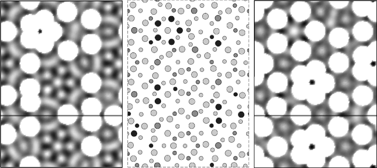
Figure 9: (a) Aluminum potential map $U_{\rm Al}({\bf r})$ in the TM poor layer. The double line shows the intersection with the $z$-slice in Fig. 10. (b)The central image shows the actual atomic coordinates under RMR. Small circles represent atoms in the TM rich layer, which will become the mirror later under period doubling. Larger circles are in the TM poor layer, which will pucker under period doubling. (c) Al potential map in the TM-rich layer.

Figure 10: A slice of the Al potential map along the $c$ direction of the same configuration as Fig. 9. The middle portion is aligned on an edge shared by two 13Å decagons. The top double line shows intersection with the cut in the right image of Fig. 9 while the bottom double line shows the intersection with the left image. At bottom, the color/shade scale (in eV) is given for all our Al potential maps.

Here we introduce a general framework to predict or rationalize the optimum positions of Al atoms, independent of the fixed-site list. It relies on the assertion made in Sec. II.2.1: one first places the transition metals (with their long-range interactions) into a sort of rigid quasilattice, and then optimizes the arrangement of Al (with their weak mutual interactions) around the TMs. To make this scenario quantitative we introduce the Al potential function $U_{\rm Al}({\bf r})$:

$$U_{\rm Al}({\bf r})\equiv\sum_{{\bf r}^{\prime}}V_{\rm AlCo}({\bf r}-{\bf r}^{\prime})+\sum_{{\bf r}^{\prime\prime}}V_{\rm AlNi}({\bf r}-{\bf r}^{\prime\prime}),$$ (2)

where $\{{\bf r}^{\prime}\}$ and $\{{\bf r}^{\prime\prime}\}$ are Co and Ni sites. This is directly analogous to the potential (for a test charge) in electrostatics, with the replacement electron $\to$ Al atom, and Coulomb potential $\to$ pair potentials. It is convenient to study the potential based on ideal positions for all transition metals while omitting any Al. FN-AlpotwithAl

Figs. 9 and  10 show two dimensional slices (in planes of local mirror symmetry) with the energies $U_{\rm Al}({\bf r})$ depicted grayscale. The $U_{\rm Al}({\bf r})$ functions plotted in this paper were produced for ${\bf r}$ on a discrete grid of points covering the unit cell, taking the TM positions in a low-energy configuration from the 4.0Å-edge (bilayer) fixed-site Monte Carlo simulation (Sec. III). This had first been put through RMR: the only effect on the Al potential map is to make it slightly more realistic, on account of the small displacements the TM atoms undergo in response to the “typical” Al distribution. The gray scale representing energy was cut off at a maximum around $+1$ Ryd to hide the large (and irrelevant) variations of $U_{\rm Al}({\bf r})$ inside the hard core of each TM.

How is the potential function interpreted to yield a set of Al sites? We start by noticing $U_{\rm Al}({\bf r})$ has a set of rather sharp and deep local minima; each is where several spheres coincide, representing minima of Al-TM potentials around different TM atoms. Each sharp well, starting with the deepest, should get filled with one Al atom. (When minima are separated by less than $\sim 4$Å, we must take into account the significant Al-Al interaction, but this is not a serious worry for this stage, since these deep minima are well isolated.) The Al sites filled in this fashion include the central atom and ring 1 of the 13Å decagon  cluster (at center of Fig. 9(c) and (a), respectively), or the analogous atoms in the Star cluster  (upper left in Fig. 9(a) and (c), respectively), as well as five of the ring 2 Al atoms (Fig. 9(c) center). FN-anisowell

The sites associated with single, deep wells were easily discovered without the help of the Al potential map: they are the unproblematic Al atoms in the fixed-site ideal structure (e.g., Al in ring 1 and 2 of the 13Å D ) that were obvious even in our first stage simulations. The potential map offers the following advantages over simulation: (i) it helps explain the structure from microscopics; (ii) it shows the energy barriers for an Al atom to pass between different local minima, which illuminates how Al atoms diffuse between sites during MD and relaxation; (iii) it can locate potential minima that lie outside of the atomic layers; (iv) it reveals potential wells which are moderately deep, but extended rather than sharp, which require more sophisticated treatment (Sec. V.3).

The Al potential map has a complementary relationship to another diagnostic, the “site energies” described in Sec. III.4.3, below. The former identifies good sites that are currently not occupied; the latter identifies unfavorable sites that currently are occupied. Together, they may be used to guide modifications by hand of idealized structures, so as to improve the energies.

V.3 Channels and puckering

The isolated deep wells of $U_{\rm Al}({\bf r})$ do not accomodate all the Al atoms. Indeed one-dimensional “channels” are evident, along which the Al potential is low and comparatively flat. Channels appear between two columns of TM (especially Co) sitting in alternate layers, as shown in Fig. 11 (a); the TM are the white disks in the middle of Fig. 10. These TM columns typically lie (in projection) on adjacent vertices of the 4Å-edge tiling. Looking at Fig. 10, a vertical slice through the periodic layers, we see how the Al has a potential trough which appears in the center as a vertical chain of dark triangles, pointing in alternating directions. The track of the channel bottom roughly consists of line segments forming a “zigzag” pattern, so as to connect the ideal Al sites that fall between the Co chains in each layer. [Fig. 11 (a) shows how, wherever the channel crosses an atom layer, it passes through an ideal Al site that is nearly at the minimum of three Al-Co potentials.] One expects Al atoms would be comparatively free to slide along such a channel. Our plots of $U_{\rm Al}$ are complementary to those of the time-averaged Al density in a molecular dynamics simulation in Ref. alnico02, , from which “channels” were originally inferred to occur (in the “basic Ni” structure.)

V.4 Origin of puckering in channels

In such a “channel”, the TM interactions do not suffice to fix Al sites. We must take Al-Al interactions into account in order to predict the Al occupation. We start with the Al potential function $U_{\rm Al}({\bf r})$ defined in Eq. (2). Let us approximate a channel with a one-dimensional vertical track parametrized by $z$. As evident in Fig. 11(b), the Al potential variation along the trough is well modeled by

$$U(z)=U_{0}-U_{c/2}\cos(4\pi z/c)+\sigma U_{c}\cos(2\pi z/c)$$ (3)

Here $\sigma\equiv+1$ (resp. $-1$) in (3), if the distant Co atoms are in even (resp. odd) layers. From plots like Fig. 11(b) one can read off $U_{c/2}\approx$ 3 eV and $U_{c}\approx$ 2.5 eV FN-U0value .

Let us explain the coefficient $U_{c/2}$ in (3); for simplicity, we neglect $U_{c}$ until Subsec. C.2. If the adjacent TM columns were all Co, and we included only interactions with them, their twofold screw symmetry would guarantee $U(z)$ has period $c/2$, modeled by the first term of (3). (Nearby Al in non-channel sites have the same symmetry.) Note that along the track, the minima of $U_{\rm Al}(z)$ lie right at the level of each atom layer. (Those locations are equidistant from three Co atoms at $R\approx 2.5$Å, the very strong minimum of $V_{\rm Al-Co}(r)$.) This explains the period and sign of the first non-constant term.

Conceivably, in some materials puckering could arise because the single-Al potential would have minima out of the atom layers; but that is not the case in Al-Co-Ni, so puckering must indeed be a consequence of the short range Al-Al repulsions (combined with $U_{\rm Al}({\bf r})$).

If both local minima were occupied in each bilayer , the Al-Al spacing would be not much more than $c/2\approx 2.0$Å, which is far too close; on the other hand, if only the best minimum in a each bilayer was occupied, and no other Al sat close to a channel, the total Al content would be too small. The solution is that there is room for three Al to fit in every two bilayers, as shown in Fig. 11(a). Since this makes the period to be $2c$, it is a symmetry breaking in each channel. The mean vertical spacing $2c/3\approx 2.72$Å is a bit closer than the Al-Al hardcore radius (see Table 1]) so the Al-Al forces are probably dominant.

Mathematical details are worked through in Appendix C.

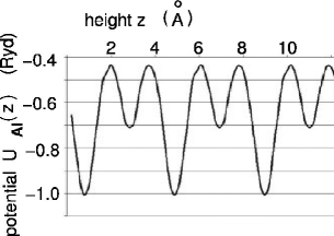
Figure 11: (a). Schematic of a channel (shaded zigzag line) between two columns of Co atoms. The Al in each channel are close enough to feel a strong mutual repulsion (arrows). (b). The Al potential energy (in Rydbergs)] along the bottom of an actual puckering channel.

Mathematical details – how the collective energy of three atoms in a channel depend on their collective position – are worked through in Appendix C. The $U_{c/2}$ term favors atoms to sit in layers. The $U_{c}$ term (as shown in the appendix) favors an individual atom to avoid the layer which is (locally) TM-rich, but when there are three atoms it favors one of them to sit in that layer, which is a point of local $z$ mirror symmetry in that channel. The result is that if a layer is globally TM-rich, it becomes a global mirror symmetry plane.

We have been deriving the configuration of a channel assuming it has a fixed number of Al atoms. Actually, of course, this number is variable. The optimum occupancy of each channel must be a function of the Al chemical potential; equivalently (in our simulations with fixed Al content) it is the result of competition with competing kinds of Al site (as measured by the site-energies). It will certainly change as a function of TM composition (changing the number of Co columns) and the total Al density (since a home must be found for every Al atom).

V.4.1 Comparison to fixed-site results

It is profitable to revisit the ideal-site models (Sec. IV) with the “channel” picture of the Al placement. All of those variable Al’s, e.g. those constituting ring “2.5” in the 13Å D, were in fact channel Al. However, in the ideal-site models they were accomodated with a periodicity $c$ everywhere: how could that work, seeing that some channels would have to fit in four Al atoms? The answer is that the mirror-layer Al’s are all in positions offset from channels, like the merged-Al site to be discussed in Sec VII.2. They are never in line with the Al in puckering layers (which don’t pucker in a fixed-site approximation), and the extra $xy$ displacement allows the mirror-layer Al to be accomodated without puckering. Such unpuckered configurations of the puckering units are observed to compete with the puckered configurations in actual simulations using RMR (see Sec. VII).

VI Long Range Order of 13Å D  orientations

In referring to the “orientation” of the 13Å decagon, we have always meant that of its Al₆Co₅ core, since the rest of the cluster, as laid out in Sec. III.2, is ten-fold screw symmetric: only the occupation of ring 1, and level of the Al atom at the center, break the symmetry. The orientation relationship of neighboring 13Å Ds  is essential because this was a prerequisite for extending our simulation results to a full-fledged decoration model (Sec. IV), and because it is tied to the differentiation of layers into “mirror” and “puckered” layers, once relaxation is allowed in a structure with periodicity four (or more)layers (Sec. V).

The ring 1 atoms from adjacent clusters are basically too distant to have a significant direct interaction: the shortest interatomic distance between the respective first rings is $2\cos 18^{\circ}\tau a_{0}\approx 7.7$Å, whereas our potentials were cut off around 7Å. Hence we must look for more subtle, indirect mechanisms to favor a relative orientation. Indeed, we have already encountered various ways the positions of the Al atoms in rings 2.5 and 3, or the substitution of Co(3) by Ni(3), is modulated by the core and thus reduces the symmetry of the outer portion of the 13Å decagon(see Secs. III.5, IV.2.2, and C.2 in particular).

The interaction must be mediated by other atoms in one of two possible ways. Firstly, neighboring TM atoms in the Star clusters  interact with each other and also respond to the first-ring orientations of adjoining 13Å decagons: we suggest this is the origin of the “antiferromagnetic” term (Subsec. VI.3.1) Secondly, the variable Al atoms in rings 2.5 and 3 are within range of ring 1 of both clusters. This contribution appears to favor “ferromagnetic” order (Subsec. VI.3.2) and is probably the more important one, both for the fixed site-list and for the relaxed, puckered structures with $c^{\prime}\approx 8.32$Å.

VI.1 Effective Ising Hamiltonian for orientations

Let us formulate the problem as an Ising model. We take as given a fixed network of $N_{D}$ 13Å decagons  placed on the “large” vertices of some configuration of binary-tiling rhombi. Each 13Å D  may have either orientation, which is labeled by an Ising spin $\sigma_{i}=\pm 1$ associated with that 13Å D. This does not unspecify all the atoms: there are options in the ring 2.5/ring 3 Al atoms, explained at length in Secs. IV.2 and IV.3, as well as TM atoms (especially in the Star clusters). For each of the $2^{N_{D}}$ possible combinations of $\{\sigma_{i}\}$, we define the orientation effective Hamiltonian, ${{\cal H}_{\rm or}}(\{\sigma_{i}\})$, to be the minimum energy after all those other degrees of freedom are optimized. FN-rotateDec We presume the orientation effective Hamiltonian is well approximated by an Ising model,

$${{\cal H}_{\rm or}}=-\sum_{\langle ij\rangle}{{\cal J}^{\rm or}}\sigma_{i}\sigma_{j},$$ (4)

where $\langle ij\rangle$ means each nearest-neighbor pair is included once.

If ${{\cal J}^{\rm or}}>0$, the ground state obviously has $\{\sigma_{i}\}$ all the same (clusters oriented identically), which we call “ferromgnetic” (FM) in the Ising model language. If ${{\cal J}^{\rm or}}<0$, it favors an “antiferromagnetic” (AF, also called “alternating”) arrangement in which neighboring clusters always have opposite orientations; that is possible, however, only if the 13Å D  cluster network is bipartite. That is not always the case on the Binary tiling – e.g. groups of five 13Å Ds  can form pentagons – but in both our simulation cells, the network happens to be bipartite.

In the rest of this section, we first report numerical studies of the energy differences between different arrangements, and then give physical explanations in terms of the pair potentials and of structure motifs (identified in previous sections). There is one story for the fixed-site simulations, and a different one for the (physically pertinent) relaxed and MD-annealed simulations. Another complication is that the answers depend on the overall density. Finally, the results show a strong dependence on the particular simulation cell being used. [We used both the standard 32$\times$23 cell and also the “W-phase” (40$\times$23) cell.]

VI.2 Orientation dependent energies (numerical)

For the numerical calculation, our procedure was to perform a series of Monte Carlo runs given FM orientations and a similar series under the same conditions for AF orientations, recording the lowest energy from each run (which is our empirical approximation of ${{\cal H}_{\rm or}}$, as just defined). We average over tens of runs, since the run-to-run fluctuation usually exceeds the AF/FM energy difference. Simulations were done for fixed-site (4Å tiling) Monte Carlo on the 32$\times$23 tiling as well as the W-phase tiling, and also with the “RMR” procedure (relaxation after MD annealing).

It was simple to constrain the orientations of each cluster. Recalled that in the rhombus decoration for our 4Å MC simulations (Sec. III.5), every 13Å D cluster is forced in a particular orientation by the five Fat 4Å rhombi that (with five Thin rhombi) make up the decagon of 4Å tiles. In particular, only one of the two layers is even available as a candidate site for the central Al atom.

The results are given in Table 5. Let $E_{\rm av}\equiv(E_{\rm AF}+E_{\rm FM})/2N_{\rm at}$, where $E_{\rm AF}$ and $E_{\rm FM}$ are the total energies for AF and FM orientations, respectively. Also, $E_{\rm diff}\equiv(E_{\rm AF}-E_{\rm FM})/N_{D}$, where $N_{D}$ is the number of 13Å decagonsper cell For these particular cells, in which neighbors are always opposite in the AF case, we can immediately extract ${{\cal J}^{\rm or}}=2E_{\rm diff}/{\bar{Z}}$, where ${\bar{Z}}$ is the average coordination number of the cluster network. (Note ${\bar{Z}}=3$ in the 32$\times$23 tiling and ${\bar{Z}}=2$ in the “W-phase” tiling, so ${{\cal J}^{\rm or}}$ is equal to the numbers in columns 5 or 6, or the number in column 3 divided by 1.5).

Consider first the fixed-site simulations. In the 32$\times$23 cell we had $E_{\rm FM}<E_{\rm AF}$ for $0.068$AA${}^{-3}<\rho<0.074$AA^-3 That is the whole range of physically reasonable densities; at higher or lower densities, $E_{\rm AF}<E_{\rm FM}$ apparently. (Of our cells, the 32$\times$23 is the closest approximant to fivefold symmetry, i.e. zero perp-space strain.) On the other hand, in the W-phase cell, we see $E_{\rm AF}$ was always lowest – though for $\rho\approx 0.070$AA^-3, $E_{\rm FM}$ was nearly as low. In other words, the concentration dependence is similar in both cases, except

$${{\cal J}^{\rm or}}(\text{W cell})\approx{{\cal J}^{\rm or}}(32\times 23\text{cell})-0.2{\rm eV}.$$ (5)

On the other hand, when the relaxed energies are compared, we found $E_{\rm FM}<E_{\rm AF}$ in all cells and at all realistic densities. In all cases, the interaction ${{\cal J}^{\rm or}}$ is of order $0.1$ eV.

	32$\times$23		W-cell		W-cell	(rel.)
$\rho$	$E_{\rm av}$	$E_{\rm diff}$	$E_{\rm av}$	$E_{\rm diff}$	$E_{\rm av}$	$E_{\rm diff}$
(Å-3)	(eV/at)	(eV)	(eV/at)	(eV)	(eV/at)	(eV)
0.66	$-0.471$	$-0.101$	–	–	–	–
0.68	$-0.453$	$-0.259$	$-0.447$	$-0.007$	–	–
0.70	$-0.430$	0.181	$-0.431$	$-0.123$	$-0.561$	0.1
0.71	$-0.414$	0.197	$-0.410$	$-0.083$	$-0.5445$	0.2
0.72	$-0.395$	0.142	$-0.394$	$-0.089$	$-0.5365$	0.2
0.74	$-0.348$	0.012	$-0.335$	$-0.143$	–	–

Table 5: Energies depending on 13Å decagon  orientations, as a function of number density $\rho$. Here $E_{\rm av}$ is the mean energy/atom [averaged over the cases of alternating (AFM) and identical (FM) orientations]. Also, $E_{\rm diff}$ is the energy cost (per 13Å decagon) of opposite orientations. The number of atoms in the simulation cell is $N_{\rm at}=207$ for the 32$\times$23 simulation cell and $N_{\rm at}=268$ for the W-phase (40$\times$23) cell, while the number of clusters $N_{D}=4$ for both cells. The first four columns are fixed-site simulations, the last two columns were relaxed after MD.

VI.3 Explanations of orientation interactions

Now let us try to explain the above results. In the fixed-site case, the data indicate the sign of $E_{\rm diff}$ – i.e., the effective interaction – varies with composition. It suggests ${{\cal J}^{\rm or}}$ (for the fixed-site case) is a sum of competing terms of opposite sign, and we indeed identified both an FM and an AF contribution (below). The relaxed case is simpler, since the result is more straightforwardly FM.

The enormous difference, in the fixed-site simulations, between the 32$\times$23 cell and the W-phase cell, is ascribed to the quite different relative ratio of 13Å Ds  to Star clusters  in the respective cells. That means that, if the stoichiometry is constrained to be the same, the actual TM content of the Star clusters  is quite different, which presumably affects the interaction term described next.

VI.3.1 “Antiferromagnetic” cluster interaction via Star clusters

We use Decoration II (Sec. IV.5). Let us assume each nearest-neighbor pair of Ni atoms in a Star cluster  has a repulsive energy $V_{\rm Ni}$. (This distance is around 2.9Å, which is not very good with the Ni-Ni potential: see Table 1.) How does this energy depends implicitly on the orientations of nearby 13Å decagons?

First, where a NiNi pair is present on an overlapping of two Star clusters, it always sits at the center of a Thin rhombus of the 10.5Å-edge Binary tiling. In this environment it can be shown that we get exactly $2V_{\rm Ni}$ from Ni pairs in the respective rings, independent of the orientations of the 13Å D’s centered of the far tips of that Thin rhombus, so this contribution is an uninteresting constant.

Otherwise, it can be shown that every pair of adjoining 13Å decagons, with the same (FM) orientations, creates one Ni-Ni nearest neighbor costing an additional $V_{\rm Ni}$ (not present in case of AF orientations). That gives ${{\cal J}^{\rm or}}=-V_{\rm Ni}$, favoring AF arrangement.

Notice that if the TM content were to be changed, there would be additional opportunities for optimizing the Ni arrangement in the Star cluster. Thus the effective interaction of 13Å decagon  orientations may involve the $\sigma_{i}$ for all 13Å decagons surrounding the Star cluster. In that case, it is not clear if the effective interaction remains pairwise, nor whether it remains AF in sign.

VI.3.2 “Ferromagnetic” cluster interactions via Al channels

Clusters want to have the same orientation for about the same reason that two steel balls, rolling on a mattress, want to be at the same place. (Here TM’s in the clusters distort Al atoms in channels in the same way the steel balls distort a mattress.) We can understand it mathematically in terms of Eq. (refeq:Uz). When there are two distant TM columns near a channel in layers labeled by $\sigma_{i}$, $\sigma_{j}$, then the second coefficient in (3) becomes $(\sigma_{i}+\sigma_{j})U_{c}$. In the fixed-site case, when each channel has only one Al atom per bilayer strictly speaking, its position will be determined by minimizing (3). The lowest energy is a term nearly independent of $\sigma_{i}$ plus $-U_{c}|\sigma_{i}+\sigma_{j}|$, which is the same as $-U_{c}(1+\sigma_{i}\sigma_{j})$ when $\sigma_{i}=\pm 1$, so we read off ${{\cal J}^{\rm or}}=-|U_{c}|$ favoring the “FM” relation.

In the puckering case, a generalization of the last term of (10) is proportional to $-(\sigma_{i}+\sigma_{j})^{2}$, so we obtain a cross-term proportional to $-\sigma_{i}\sigma_{j}$ again favoring “ferromagnetism.”

Now, ${V_{1}}^{\prime\prime}$ depends very sensitively on how close $2c/3$ is to the Al-Al hardcore radius, and consequently so does ${{\cal J}^{\rm or}}$. A corollary is that small changes in the layer spacing can have large effects on the orientation order.

VII Systematics of the puckering pattern

We now return to the thread of Sec. V: there we understood puckering within an isolated “channel” between two columns of TM (usually Co) atoms in alternating layers A filled channel contains three Al atoms per four atomic layers. one in a mirror plane and two atoms assigned to the “puckered” layers above and below it. This picture does not specify which of the two mirror layers gets occupied (which determines the out-of-layer displacements of the other two Al): this is a local twofold symmetry breaking. In this section, we address the puckering correlations, in particular the relation of the local pattern to the local geometry of tile packing/cluster network, and whether long range order of the symmetry breaking can be propagated. An effective Ising model helps define the question, but is inadequate to answer it. Instead, we focus on “puckering units” defined as the (up to five) channels surrounding a Co column, and their Al atoms, which are subject to strong steric constraints.

To explore the puckering patterns, we performed RMR on two bilayers, starting from a (4Å  periodic) fixed-site configuration (of Sec. IV), using the decoration of Fig. 7 Several independent relaxations (with MD annealing from $T=$700 K to $T=0$ in stages of 50K) in the “W-phase” unit cell. gave substantially similar arrangements (Fig. 12). (Note many channels had $n_{\alpha}=4$ Al, suggesting either the Al content was too large, or the MD time was insufficient to allow Al atoms to diffuse between channels. ) We will analyze (in Subsec. VII.3) the typical patterns in the puckering units, and discover the key role of Star clusters  in organizing longer-ranged correlations.

VII.1 Ising-spin variables and channel occupancies

One way to formulate the puckering problem is to represent the symmetry breaking in each Al channel by an Ising spin-like variable FN-pucksigma ${\mu}_{\alpha}=\pm 1$. (Here the index $\alpha$ runs over all ${N^{ch}}$ distinct channels.) Arbitrarily designate one of the mirror layers as layer 0, consistently throughout the system. Where layer 0 is occupied and layer 1 puckers upward, we define ${\mu}_{\alpha}\equiv+1$; where layer 2 is occupied and layer 1 puckers downwards, ${\mu}_{\alpha}\equiv-1$. (Layer 3 always puckers in the direction opposite to layer 1.) An Ising value ${\mu}_{\alpha}=+1$ corresponds on Fig. 12 to a $+$ symbol and a blackened circle, usually on a 4Å tile edge and always between a pair of Co (identified in the lower panel) in different layers; similarly ${\mu}_{\alpha}=-1$ appears as an $\times$ symbol and a white circle.

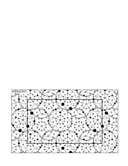
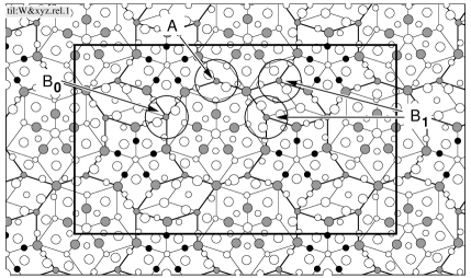
Figure 12: Puckering of 8Å structure in a simulation in the W-phase cell (after RMR relaxation from a 4Å periodic structure, a realization of the same decoration as in Fig. 7. (a). Puckering pattern, showing three of the four layers. The “$\times$” and “$+$” symbols represent, respectively, atoms in mirror layers 0 and 2. White (resp. black) filled circles are atoms in puckered layer 1, deviating in the plus (resp. minus) sense, where the circle radius is proportional to the displacement; gray circles have small puckering displacements. Puckered layer 3 has atoms in the same places (apart from a handful of defects), each deviating in the opposite sense from layer 1. (b). One bilayer, showing relaxed positions and atom chemistry with our usual conventions. The other bilayer is similar, except at atoms where the mirror layers differ; those are always Al and can be identified from places in (a) where “$\times$” and “$+$” do not overlay. Locations of puckering units are shown by circles, labeled $A$, $B_{0}$, and $B_{1}$ according to their environment in the tiling, as described in Sec. VII.3.1.

Now imagine computing the total energy for every one of the $2^{{N^{ch}}}$ channel configurations. The result, one hopes, is well approximated using pair interactions between nearby channels, giving an effective “Ising model” Hamiltonian

$${{\cal H}_{\rm puck}}=\sum_{\alpha\beta}{{\cal J}^{\rm puck}_{\alpha\beta}}{\mu}_{\alpha}{\mu}_{\beta}.$$ (6)

The effective interactions $\{{{\cal J}^{\rm puck}_{\alpha\beta}}\}$ would depend on the locations of channels $\alpha$ and $\beta$ relative to 13Å decagon clusters, and also on the choice of TM occupancy of nearby sites (Ni versus Co in many places, but also Ni versus Al in Star clusters.) The final ground state would be determined by minimizing (6).

The real story is more complex. We have presupposed a fixed set of channels, each containing $n_{\alpha}=3$ Al and thus having an Ising “spin” degree of freedom. But if an Al atom is moved in or out of a channel (so $n_{\alpha}$ = 2 or 4), the atoms are locked in unpuckered layers. In the case $n_{\alpha}=2$, both Al go into a puckering layer since we found (see AppendixC) the Al potential is lower there, but they need to pucker only negligibly (in response to distant Al). In the case $n_{\alpha}=4$, some of the Al must deviate sideways and the atom sites are essentially an arrangement (using “ring 2.5”) of the fixed-site structure of Sec. IV, so again there is no local symmetry-breaking by puckering; in either case, there is no longer a spin ${\mu}_{\alpha}$ at that place. (Of course, a new ${\mu}_{\beta}$ will have appeared somewhere else, if $n_{\beta}=3$ now as a consequence of the move.)

Thus, the channel occupation numbers $n_{\alpha}$ are a separate degree of freedom. We presume that, in most channels, the optimum is $n_{\alpha}=3$ and the energy cost of $n_{\alpha}$ deviating is much larger than the ${\mu}_{\alpha}$-${\mu}_{\beta}$ interaction. But when the total Al available to channels is (say) less than $3{N^{ch}}$, this forces a “doping” by $n_{\alpha}=2$ channels, and there are many nearly degenerate ways to place them. Since the puckering effective Hamiltonian depends on the configuration $\{n_{\alpha}\}$, we may very easily find that two separated ${\mu}_{\alpha}$ variables are favored to be the same or opposite, depending on the occupancy of some intervening channel. (The location of channels with puckering also depends on the presence of Ni neighbors to the Co atoms in the central column; that is also highly sensitive to composition and density, see Sec. III.6)

Furthermore, under our protocol – MD simulations at moderate temperatures, starting from an arrangement on ideal sites – the occupancies $\{n_{\alpha}\}$ are mainly quenched, after the ring 2.5/ring 3 Al atoms have found their way into nearby channels; diffusion of Al from one puckering unit to the next seems to be suppressed. Consequently we cannot trust MD simulation to discover the optimum arrangement; since the $\{{{\cal J}^{\rm puck}_{\alpha\beta}}\}$ are not only random but frustrated, the puckering effective Hamiltonian in fact describes a spin glass.

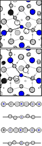
Figure 13: Puckering in a typical 2.45Å star. Colored circles (using the same conventions for species and layer) are the optimum configuration assuming a bilayer ($c\approx 4$Å) period, given ideal quasilattice sites as used in lattice-gas simulation. Note that channel interpretation is valid here as well. If we draw lines from the center of the 2.45Å star to the nearest TM atoms (3 are already drawn as 13Å D edges, four channel formations can be seen. (a,b) Each image is two layers in a structure with 4-layer ($c\approx 8$Å) stacking period. The large empty circles represent locations achieved after relaxation. This particular 2.45 Å star is on a vertex shared by two 4.0Å decagons (solid lines). (c). Side view; the $z$-direction scale is increased by a factor of $\sim$1.44. Six TM atoms are depicted from each bilayer as X’s. Faded indicates that the TM atom lies behind the Al atom in this projection.

VII.2 Puckering units

A description in terms of independent channels is problematic not only because of their variable occupation, but also (as we shall see) not every set of $\{\mu_{\alpha}\}$ values is meaningful owing to steric constraints.

Instead, our approach to make sense of the puckering pattern is to define the “puckering unit” (Fig. 13), which consists of all channels (usually five) centered on the same Co column, and their Al contents. In our models, each puckering unit is centered on a 13Å decagon  vertex and occupies one of the 2.45Å HBS tiles introduced in Sec. IV.2, which encircle the decagon center in the DHBS picture. In fact, the puckering units are always on 13Å D  corners aligned (in projection) with the five core Co atoms, and the 2.45Å tile is usually a Star. (This is a consequence of how the latter Co atoms determine mirror layers, as expained in Sec. V.3. The strong interactions between adjacent channels a small menu of configurations for each puckering unit, from which one can build the larger-scale patterns of $\{{\mu}_{\alpha}\}$ in the structure.

Now, the channels around one Co column come very close in the ideal mirror-layer Al sites are $2\tau^{-1}\sin(2\pi/10)a_{0}=$ 1.79Å from each other and cannot simultaneously be occupied. – adjacent channels must have opposite signs of ${\mu}_{\alpha}$. But if (as usual) there are five channels, this alternation is frustrated. The resolution is that two adjacent ${\mu}$ values are the same, but the two mirror-layer Al sites get merged into one Al at the midpoint. There is practically zero cost in the Al potential for such a deviation: Fig. 9(c) shows the channels are actually connected by ring-shaped troughs in the mirror layers, which include the fused Al sites. As for the puckering-layer Al atoms, since they sit farther from the central axis, there is no steric rule against adjacent ones having the same puckering sign ${\mu}_{\alpha}$.

Thus, in a fully puckered configuration, a puckering unit has room for only two Al atoms in either mirror layer, a total of four. These atoms generally arrange themselves into a motif we call a “crooked cross” (see Fig. 13). In projection, one arm of the cross (consisting of two channel Al sites) is bent to an angle $2(2\pi/5)$; it is bisected by a straight arm, consisting of a channel site on one side and a merged site opposite to it. [If there were just four channels, both arms of the cross are liable to be bent at angle $2(2\pi/5).]$

VII.3 Configurations in puckering units

In this subsection, we first classify puckering units according to their environment with respect to the 13Å decagon-Star cluster  geometry (or equivalently the 10.4Å-edge Binary tiling); we also classify the resulting patterns of Al occupancy and puckering in each puckering unit. Then, studying plots like Fig. 12 from separate RMR relaxations, we count the frequency of puckering patterns in each kind of location; indeed, the patterns are nearly determined by the environments (especially if the placement of TM atoms in nearby Star clusters  is taken into account).

Besides the W-cell, we also performed RMR relaxations (starting from a different decoration) in the 32$\times$ 23 cell (not shown); in this case, the initial fixed-site structure was the result of a lattice-gas MC simulation (using 4Å tile decoration), rather than an ideal decoration rule. The behavior of puckering centers was different in the two approximants; one reason is that our 32$\times$23 structure (with a total point density 0.068Å${}^{{}_{3}}$) is packed with a much lower density of Al atoms than the W-cell (at density 0.070Å${}^{{}_{3}}$).

VII.3.1 Nomenclature for puckering units

We categorize the puckering-unit centers on the 13Å decagon  edge as type $A$, $B_{0}$, $B_{1}$, or $B_{2}$, according to where they fall on edges of the 10Å-edge Binary Tiling. Type “$A$” sits on the interior of a Fat rhombus of the Binary tiling; more important, it is a vertex shared between two 13Å decagons. A type $B$ site is along a ray connecting the 13Å D  center to that of a Star cluster, which is always an odd Star cluster  in the assumed scheme of orienting the cluster centers. That ray is an edge of the 10.4Å Binary tiling; the cases that it goes between Thin/Thin, Fat/Thin, or Fat/Fat rhombi define environments $B_{0}$, $B_{1}$, and $B_{2}$, respectively. The environment $B_{k}$ has at least $5-k$ columns of TM neighbors (in the other layer) from the 13Å D  itself, each of which creates one channel in between. It will have more channels (up to five), whenever TM occupying the right candidate-TM site(s) of the neighboring Star cluster  supplies the necessary second TM column.

In projection, the positions of the $m$ mirror-layer atoms next to the central Co (appearing as $+$ or $\times$ symbols in Fig. 12) are the best way to visualize the configuration adoped by a puckering unit; So, we label the possible Al configurations in a puckering unit by a letter “$p$” or “$u$” for “puckered” or “unpuckered”, followed by the number $m$. “Unpuckered” means all the $+$ and $\times$ symbols are superposed in pairs (sometimes the pairs are not quite lined up); “puckered” means the Al in one mirror layer is missing, in at least one place. Farther out from the puckering unit’s center, there are always two puckered-layer Al sites in every channel, each of which follows the closest mirror-layer Al site(s): displaced in a determined sense (large black or white circles in the figure) if the latter is puckered, undisplaced if it is not.

Finally, we sometimes add a $+$ or $-$ superscript to the label, to record the parity of the puckering sense under the (vertical) mirror plane of the 13Å decagonthat passes through the 13Å D  center and the Co puckering-unit center. (The $-$ parity appears more frequently.) Thus, a typical shorthand symbol is “p$4+$”. Still, some of our labels refer to more than one configuration. A unique way to name any puckering-unit configuration is given in Appendix D.

VII.3.2 Results: statistics of puckering units

Our observations need to be prefaced by a caution. The idealized decoration, when applied to different approximants, will lead – in view of the locally inhomogeneous densities of species and of the binding energy in our model – to differing densities and compositions for the approximants, and may destabilize some finite approximants with a decoration that would be stable in the thermodynamic limit. As a corollary, if the same composition and density is forced on the different approximants, it may occur e.g. that one of them is overpacked with Al atoms and the other one is underpacked.

Location	Cell	Number	Frequency
type		in cell	Ni	$p4$	$\quad p5$	$u6$
$A$	W-cell	4	0	0	0.6	0.4
$A$	32$\times$23	6	0	0.6	0.4	0
$B_{0}$	W-cell	4	0	0.9	0.1	0
$B_{1}$	W-cell	8	0	0.1	0.5	0.4
$B_{1}$	32$\times$23	4	0.25	0.5	0.2	0.3
$B_{2}$	32$\times$23	4	0.75	0	0.2	0.8

Table 6: Frequency of local puckering configurations ($p4$, $p5$, and $u6$) in puckering units, classified according to location type in the large tiling; these add to 1. Column “Ni” gives fraction where the central Co has a nearest-neighbor Ni atom. The total number of distinct puckering units was 16 in the W-cell and 14 in the 32$\times$23 cell. Each frequency is based on 20-50 examples of the puckering unit, in different places within the cell and/or from different runs.

Table 6 summarizes the statistics we found; they should be taken only as rough numbers, especially as runs taken under different conditions were combined. Each column lumps together several distinct patterns, distinguishable by the long names from Appendix D (if not by parity).

In the “$A$” environment, half the units were $p5$, and the rest were $p4$ or $u6$, depending on Al density. Both $B_{0}$ and $B_{1}$ environments show a “crooked cross” pattern, in two variants oriented differently with respect to the 13Å D: $B_{0}$ has $p4^{-}$ while $B_{1}$ has $p4^{+}$ Actually, in the $B_{1}$ case, Al in the neighboring candidate-TM site in an Odd Star cluster  (which counts as a merged mirror-layer channel site) strongly tends to be unpuckered: thus the crooked-cross gets modified to $p5^{+}$. Finally, the “$B_{2}$” environment is typically an unpuckered $u6$.

However, the overwhelming factor affecting puckering is whether the central Co has a Ni neighbor in the candidate-TM site of an adjoining Odd Star cluster, which is a merged-type site if there are channels on that side. In any case, the Ni always occupies both mirror-layer sites, so that tends to favor unpuckered channels all around this puckering unit. A “$B_{2}$” environment is typically unpuckered mainly because it typically has a Ni neighbor (at least in the 32$\times$23 cell). Note also that if the neighboring candidate-TM site of the odd Star cluster  is not TM, then one or both of the candidate-TM sites one step away probably is TM, which increases the number of channels in this puckering unit and (probably) makes it likelier to adopt a puckered configuration.

In Table 6, both $A$ and $B_{1}$ environments are packed with more Al in the case of the W-phase cell, reflecting its higher overall packing. Despite this, the mean occupancy $m$ is practically the same (5.0 in the W-phase cell, 4.9 in the 32$\times$23 cell). The reason is that the W-phase cell contains another environment $B_{0}$, which usually has $m=4$, while the 32$\times$23 contains $B_{2}$, which usually has $m=6$. If the overall density of Al (and hence its effective chemical potential) were set the same, we iamgine each environment type would show similar behavior in both cells.

VII.4 Puckering around Star clusters

In any Even Star cluster, there tend to be TM atoms on all ten vertices of its 4Å-edge Star tile (of the DHBS tiling): most of them are 13Å decagon  vertices, while the others are candidate-TM sites where two Star clusters  touch; as noted in Sec. III, the latter often have a TM-TM pair. If furthermore the latter sites are Co, and some candidate-TM sites of the Star cluster’s interior are also occupied by TM, then the Star vertices not on a 13Å D  become puckering centers too, and all ten exterior edges have channels. This happens in the special decoration of Fig. 7.

On the two edges meeting at a $2\pi/5$ corner, the puckering sense should be opposite due to the steric constraint. At an indented [angle $3(2\pi/5)$] corner, the sense is also opposite, i.e. the parity (with respect to the adjacent decagon) is $-$, consistent with the usual tendency (noted above). Thus, the puckering sense alternates as one passes all the way around the Even star’s exterior edges, producing a striking pattern in images of the puckering. (Such patterns are even more prominent in the real $W$(AlCoNi) structure: see Sec. VIII.)

Furthermore, when there is a chain of Star clusters  (as in the W-cell), the interaction between successive Even Star clusters  is such that their patterns have the same puckering sense. This accounts for most of channels around every 13Å decagon(all those in puckering units of types $B_{0}$ or $B_{1}$). It leaves unspecified, however, what happens along the edge shared by two 13Å decagons. The non-channel atoms nearby are perfectly symmetric under the (vertical) local mirror plane that includes the shared edge. And, following the star rule just described, the puckering sense will be opposite on the adjacent unshared edges of the respective 13Å decagons. Thus the puckering sense on the shared edge is necessarily given by a local symmetry breaking, and cannot propagate the pattern from the Star cluster  chain on one side to the Star cluster chain on the other side.

With the alternative decoration of Subsec. IV.5, the 4Å edge star would not have Co on every vertex (nor would the 13Å D, for that matter), and the puckering patterns just mentioned would, one expects, be disrupted. On the other hand, in a model built from disjoint 20Å decagons (see Appendix E), the Star cluster  chains are more extensive and might propagate a puckering sense globally. Conceivably, the puckering interactions might be strong enough to tip the balance between different placements of TM atoms (e.g. alternative decoration) or between different basic structures (e.g. the 20Å decagon structures). The approach we followed in the present work could not answer such questions, since the positions of all TM atoms (and some Al) are permanently determined at the fixed-site stage of modeling.

VIII Simulation of Experimental Approximant W(AlCoNi)

In this section, we compare our prediction with the approximant structure $W$(AlCoNi), currently the only refined Al-Co-Ni structure on the Co-rich side. The solution of of atomic positions was done by Sugiyama et al Su02 using direct methods (the SIR97 package).

VIII.1 Attempted prediction of W(AlCoNi) by simulation

For our simulation, we used the same 4Å rhombus tiling which optimizes the decagon density, as explained in Subsec. III.5.1. As inputs, we took the experimental lattice parameters $23.25$Å$\times 39.5606$Å$\times 8.16$Å and the experimental reported point density and composition. (This differs from the standard composition and point density from Sec. II.2.2 that we have used up till now in this paper.) By comparison, the decoration of Fig. 7 has atom content Al₁₈₈Co₆₀Ni₂₀, which is too rich in Co compared to real $W$(AlCoNi), while its density of $n=0.071$ Å^-3 is slightly denser than real $W$(AlCoNi) (See table 3).

The result of our discrete-site simulation – which our Fig. 7 was devised to idealize – looks quite similar (in $c$-axis projection) to the experimentally determined $W$(AlCoNi) cell. Su02 However, a significant number of Al atoms present in the diffraction refinement could not be found in our simulation result. Also, the TM arrangements in our Star clusters  do not agree with those in the W-phase.

We next apply the “relaxation-molecular dynamics-relaxation” (RMR) protocol defined in Sec. V; in the molecular dynamics portion, the temperature was initially $T$=600K and was then cooled in gradual stages to $T=$50K. The RMR structure shows the usual puckering (Sec. V) similar qualitatively to the prominent puckering of the actual approximant.

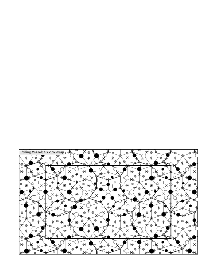
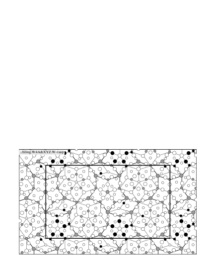
Figure 14: Puckering in the W(AlCoNi) structure, using same conventions as Fig. 12

VIII.2 Pentagonal bipyramid cluster

The actual W phase differs from our decoration (such as Fig. 7) essentially by the following modification: half of the Even Star clusters  are replaced by a new cluster which is just the “pentagonal bipyramid” (PB) cluster Hen93 ; Wid96 identified long ago in Al₁₃Co₅ (and other decagonal approximants). Whereas the original (Even) Star cluster  is Ni-rich and 4Å periodic in the stacking direction, the PB  is Al-rich and strongly puckered (so it is 8Å periodic).

One novel feature is that the apex TM atom (on the PB axis) puckers noticeably, which has not been true for any TM atoms up till now (even the ones in puckering layers, which are allowed by symmetery to pucker). In fact, the arrangement around the PB center is quite similar to that around a 2.45Å Star; indeed, the central TM column is a new kind of puckering center that is not on any 13Å decagon. The mirror-layer channel Al adopt a new puckering pattern, in which all five go to the same layer and sit in merged sites.

The model of Ref. del06, (elaborated here in Appendix E.3) adopted the PB as its fundamental cluster because, in the real $W$ phase, fivefold symmetry extends quite far from its center. We must disagree with their assignment of atoms of the innermost PB ring as mixed Al/TM: these are right in a channel, and should in fact be Al. Conceivably in a real structure, there is some disorder in the placement of the two ways of decorating Even Star clusters. Since the TM ring of the “standard” Even Star cluster(of Fig. 7) occurs in the same place as the Al ring of the PB, that would give an averaged structure as if there were Al/TM substitutions.

VIII.3 Puckering propagated by Star clusters  and PBs

Fig. 14 shows that the actual $W$-AlCoNi structure has a more pronounced and better propagated puckering pattern, as compared to our model structures such as Fig. 12. The key to this is the PB which is, in a sense, one big puckering unit. The three Al pentagons in the middle all belong to channels along the interior 4.0Å edges in the five-rhombus star containing a PB (the Al pentagon in a mirror plane consists of all merged sites). Although the edges of the 4.0Å-edge star have alternating puckering senses, just like the ordinary Even stars did, these are not the key atoms for propagating the sense, The key atoms are those mirror-layer Al visible (in the top panel of Fig. 14) just inside the tips of that five-rhombus star, which lie in the same layer as the mirror-layer Al pentagon in the middle.

These tip Al atoms correlate the PB  puckering with the adjoining Star cluster  cluster, which puckers in the same pattern discussed in Sec. VII.4, and thus propagates a well-defined puckering pattern along each chain of Star clusters  in the underlying tiling. Inside the 13Å decagons, unlike Fig. 12, the ring 2 Al atoms (not in a mirror layer) pucker strongly. Each (along with ring-2.5 Al in the same channel) adopts a sense opposite to the nearest puckering atoms from the Star clustersor PB’s: the ring-2 Al facing Star clusters  alternate while those facing PBs  all have the same sense, producing the complicated pattern of white and black circles inside the 13Å decagonsin] the top panel of Fig. 14. However, just as in the PB-less case of Sec. VII.4, it is hard to see how the pattern actually propagates from one chain of PBsand Star clusters, through the 13Å Ds, to the next chain over.

IX Discussion

In conclusion, we have carried out the most extensive prediction of a quasicrystal structure that makes minimal assumptions and combines lattice-gas Monte Carlo with relaxation and molecular dynamics. The overall story of this project is that our approach, on the one hand is fruitful at producing atomic structures with very good energies and very good local order (i.e. consistent with structural experiments). On the other hand, its application is an art rather than an algorithm, and there is no guarantee of discovering the absolute best solutions. Difficulties are to be expected especially when we must discern between variants that have similar energies, yet cannot easily transform to each other: brute-force Monte Carlo is not sufficient to overcome this energy barrier.

The “basic Co” structure turned out to involve substantially more complications than the “basic Ni” case studied previously. One measure of the complexity is that, at different places, it was convenient to introduce tilings on five different length scales (related by powers of $\tau$). Table 7 gives sort of index to the sections where they were defined or used.

There are three features of “basic Co” that made it more complex than “basic Ni”, even at the stage of modeling limited to discrete ideal sites (sections I - IV): (i) a larger cluster unit (13Å decagon), introduced in Sec. III.2; (ii) a set of sites (the ring 2.5 and 3 Al) which break the symmetry of the basic cluster; to first order, these give rise to a high degeneracy, which is broken in fairly subtle ways (Sec. IV). (iii) the orientational ordering pattern of the clusters, which strongly affects the decoration even though it involves relatively small energy differences, that depend on composition and density in complex ways (Sec. VI).

Tile edge	Tiling	Sections
2.45Å	rhombus	II.1 (Fig. 1), III.1 (Fig. 2),
	(two layers)	III.2 (Fig. 3(a) only)
2.45Å	HBS (basic Ni)	III.7
2.45Å	DHBS	III.4, IV.2 (Fig. 7),
		IV.3 (Fig. 8)
4.0Å	rhombus	III.2 (Fig. 3(b) only), III.5,
		III.4(Fig. 5 only),
		VII (Fig. 12), VII.4
4.0Å	DHBS	IV.2.3
6.5Å	DHBS	App. E.2
10.4Å	Binary	III.3 (Fig.4(c)), IV.1.2,
	(rhombus	IV.3 (Fig. 8), IV.6,  VI.1,
	or HBS)	VII.3.1, App. B.3 (Fig. 15)
17Å	any	IV.6, App. E (Fig. 17)

Table 7: Different tilings used in this paper to describe $d$(AlNiCo), with the sections (or figures) where they are referenced.

Sections V-VIII developed a second layer of simulation, the use of relaxation and molecular dynamics to obtain more realistic configurations. This turns out to make a fundamental difference in the “basic Co” case, because many of the Al atoms deviate from their fixed positions to break the 2-layer ($\sim 4$Å) stacking periodicity down to 4-layer periodicity. This happens (Sec. V) in “channels” due to columns of Co atoms that run perpendicular to the layers and are filled with three Al atoms each that define mirror planes and puckered layers. We have explained this behavior in terms of the potentials (Appendix C) – this work Gu06-ICQ9 appears to be the first time any explanation has been given for such period-doubling, a very common phenomenon of period-doubling in decagonal quasicrystals. To understand the correlations of the puckering deviations (which create the structure in well-known layers of diffuse scattering seen in decagonals), yet another framework was needed of the “puckering center”, (up to) five mutually constrained channels around a single column of Co atoms (Sec. VII).

In this latter half of the paper, two sections are included that are not specially focused on relaxation and puckering, but which could not be formulated in terms of just the fixed sites. First, in Sec. VI we found that puckering drives the clusters’ orientational order (which breaks the symmetry down to pentagonal). Second, in Sec. VIII we show that our approach goes a long way towards successfully predicting the structure of the phase $W$(AlCoNi), and in turn $W$(AlCoNi) offers additional clues for future modeling of Al-Co-Ni decagonals.

Massive as it is, this study is still far from a definitive answer about the $d$(AlCoNi) structure. Although the atomic structure we presented is unquestionably a good one, we suspect there exist competing structures (built from similar local structure) that are just as good. In part, our failure to study these is an intrinsic weakness of the initial approach via discrete site lists, when we know puckering is a key feature of the structure. But to a greater extent, it stems from small misapplications of the technique. Although we used much larger cells for the discrete simulation than in previous work alnico01 , we should have used even larger cells; furthermore, the degrees of freedom were too quickly reduced when we passed to a description based on 4Å, or really 10.4Å, tiles (Sec. III.5). These adjustments would have revealed the alternative framework based on 20Å decagon clusters (Appendix E). Based on this experience, we anticipate that future applications of the method will evade these pitfalls.

In the rest of this section, we examine some of the implications or future possibilities in more detail.

IX.1 Pitfalls of discrete site list

From some viewpoints, one may be surprised that constraining sites to atiling works at all, or suspicious whether it is transferable to pther quasicrystals. Perhaps it is that, in order to form a high-quality quasicrystal, the atomic configurations already have to be tiling-like. [The identical local pattern has to be compatible with different environment patterns.]

We still believe we it was effective to initially simulate using a 4.08Å period, in order to discover the main features, and to refine this later on. In part, this was justified by some simulations using 8.16Å periodicity, in which we saw that 4.08Å periodicity persists for a large subset of the atoms.

However, the dangerous step is eliminating sites: without care, an unjustified assumption can get built into later stages. In particular, there are subtle issues in connection with the density The candidate site list for MC lattice-gas simulations on the 4Å edge rhombi was constructed to eliminate sites that were observed to be unused in the previous stage of simulation using 2.45Å rhombi. This is valid, so long as we retain the original composition and density in the final model. Usually, however, as we grow to understand the structure better, different compositions and densities recommend themselves for the idealized model, because the modified atom decoration (i) is simple to prescribe, or (ii) is favorable energetically. In the present work, the initial explorations were conducted at a density $0.068$Å^-3, which is a bit loosely packed, whereas the idealized model of Fig. 7 at $\sim 0.070$Å^-3 may be somewhat overdense. Thus, when MC annealing of Fig. 7 fails to find any better configuration, it might be an artifact of the poverty of the candidate site list for this higher density. The moral is that the initial exploratory runs ought to be done with (at least) two densities; to ensure a conservative choice of site list in later stages, one of the densities might be higher than the expected real one (though not too high, as that would slow down the lattice-gas annealing).

Although natural, doing (almost all) our fixed-site simulations with a “standard” density and composition (see Sec. II.2 and III.1) equal to those of “basic Co” $d$-AlCoNi was an unfortunate choice. For one thing, the nominal composition and density are unlikely to match exactly those in our ultimate idealized decoration.) More importantly, even if they do match, one cannot rely on such simulations to infer the appropriate site-list for later stages, since the later stages will explore variations in density and composition. There is a chance the preferred sites for the variation already got eliminated at the earlier stage, since they were not being occupied in the initial small-tiling simulations. Instead, the initial exploratory simulation should run at a density chosen higher than the expected value, indeed higher than the largest density variation to be tried in subsequent runs. (Or, even better, at densities and compositions bracketing the expected ones.)

IX.2 Adapting the method to puckering?

Yet another reason that the “basic Co” story is more complex is that relaxation and the formation of “channels” that violate the layering (Sec. V) have more dramatic effects than they did in the “basic Ni” case alnico02 . Perhaps the reason is simply that “puckering centers” form around columns of Co atoms; they are present in both phases, but since “basic Ni” has half the density of Co atoms, its puckering centers are sufficiently separated that their interactions are unimportant. The most serious issue here is that relaxation might reverse the sign of a small energy difference between competing variants of the detailed atomic structure – we encountered such a sign reversal when comparing different cluster orientation orders (see Table 5). Thus, one must worry whether our recipe may converge to a non-optimal answer, having discarded the correct one in the early fixed-site stages. Are there any technical ways to incorporate puckering, while still using discrete Monte Carlo simulation? One may distinguish three points in our story at which one could ask for such a remedy.

The first point is in the initial small-tile stages of MC, where we would worry that we might miss a nice form of local order, due to the unphysical fixed-site and layering constraints. Obviously, this should be performed using a four-layer unit cell, but that is insufficient by itself: if atoms cannot reduce their energy by deviating off layers, the 4Å symmetry remains unbroken (as we verified by some trials). The key to improvements must be the understanding that puckering is built from an alphabet of in discrete entities – channels (Sec. V) or puckering units (Sec. VII.2) – which are put together, somewhat as tiles are put together in a tiling.

One approach, at the raw 2.45Å rhombus level, is to add a correction to the Hamiltonian which models the energy reduction that would occur under relaxation. This would have important negative contributions only in cases where atoms in adjacent layers are stacked nearly on top of each other (e.g., one of the “short bonds” recounted in Appendix B.1), but are not thus constrained by other atoms on the opposite side from the close neighbor. This would have exactly the form of a three-atom interaction. The coefficients in this effective Hamiltonian could be fitted to the relaxed energies for a database of random 2.45Å configurations.

Alternatively, we could approach the problem at the level of the 2.45Å DHBS tiling (see Sec. IV.2; this tiling has not yet used for MC for the present model system.) We found that the 2.45Å HBS tiles, each centered by a Co column, correspond closely to the puckering units. Thus, we might incorporate e.g. 2.45Å Star tiles of several different flavors, corresponding to the common puckering patterns (e.g. Table 8). Within each tile, the puckering-layer Al would be displaced, but other Al would lie strictly in layers. This would undoubtedly be a crude way to represent the continuum of possible Al positions, but the existing method is much cruder (in forcing them to lie in the layers).

A second point where we need a technical adaptation was the stage where we conducted molecular dynamics and relaxations, to obtain configurations such as Fig. 12, or relaxed energies such as those in the right columns of Table 5. We were hampered by using starting configurations that always have the wrong number of atoms in every channel: there ought to be three, but two copies of a bilayer necessarily have an even number (two or four). We worry that the channels may get stuck with random, non-optimal patterns of occupancy (see Sec. VII.1) and this may obscure any pattern that would emerge.

At this stage, it doesn’t matter greatly how well the model positions approximate the real ones, since we are not comparing energies of the unrelaxed configurations. Instead, we just need more of an ideal decoration model similar to Sec. IV, but having four layers, such that the two mirror layers differ in places. The model should admit variants, so that we could discover which rule allows for the best relaxed results.

A final stage where puckering should be represented has been reached in the “basic Ni” case alnico01 , but not yet for “basic Co”: a deterministic decoration for quite large tiles (4Å or probably larger), allowing discrete Monte Carlo simulations in which only these tiles were reshuffled. One approach that was used in Ref. Mi96b, to devise such a decoration is “constrained relaxation”, whereby all atoms in the same “orbit” (quasi-equivalent sites generated by the same decoration rule) are forced to move in the same exact manner relative to the tiles they decorate, defining a sort of consensus relaxation.

IX.3 Long-range order of the puckering pattern?

Our structure model develops very robust puckerings (Sec. V) with a 8Å period in the $c$ direction. Assuming the motifs that we discovered and built our description on, the puckering interactions are frustrated and sensitive to the Al density and to the Ni placements in Star clusters, which together (see Subsec. VII.3.2) determine which channels pucker. The disorder inherent to any real quasicrystal might introduce sufficient randomness that the Ising effective Hamiltonian of Sec. VII.1 would be a spin glass model having many almost degenerate minima. If so, our attempts to discover the true ground state are rather academic. as the real material would probably get trapped in (somewhat higher) metastable states.

Within each “channel”, the correlations should extend far in the $c$ direction; yet our tentative conclusion is that the puckering order propagates poorly within the $xy$ plane. The consequence of this would be diffuse scattering concentrated into “pancakes” in thin layers close to $q_{z}=\pi/c$ and (stronger) $3\pi/c$, midway between the Bragg layers, but rather broad in the $xy$ direction in reciprocal space.

However, the observed diffuse scattering associated with the 8Å periodicity tends to show longer in-plane correlations frey00 ; kat04 . In fact, many $d$-AlNiCo modifications propagate true long-range order of the puckering, as shown in diffraction patterns have sharp Bragg spots in the intermediate layers (that appear between the main layers associated with $c$ periodicity). So, when the real material does have long-range puckering correlations, one may wonder if it includes some motif beyond our model.

In fact, the $W$(AlCoNi) phase does propagate a well-ordered puckering, and manages this by replacing half of the even Star clusterswith another motif, the pentagonal bipyramid (see Sec.VIII.2). So, a plausible conjecture is that the PB  is the missing motif which is responsible for extended puckering correlations (in the more Co-rich modifications of Al-Co-Ni).

IX.4 Relation to decagonal Al-Co-Ni at other compositions

A variety of small-grained, apparently metastable, crystalline approximant phases are found alongside quasicrystals at compositions near $d$(Al₇₀Co₁₅Ni${}_{15})$; it was suggested that the presence of quenched-in vacancies might tilt the balance to stabilize one of the approximants against the quasicrystal grushko-approxts . The difficulty of determining stability suggests that these related phases are very close in free energy. Since the decagonal domain of the Al-Ni-Co phase diagram is bracketed by phases we studied (“basic Ni” in Ref. alnico01, ) and “basic Co” in this work), can we say more about those intermediate phases?

One clear conclusion alnico01 is that special compositions are stabilized, in large part, because each species is filling a particular type of site. Thus a small composition difference (density or stoichiometry) can cause certain orbits (classes of quasi-equivalent sites) to become occupied or to change species. At a higher level, the interactions of these atoms will then change the tile Hamiltonian of the tiles they sit on; and that can make a big difference in how these tiles freeze into supertiles at even larger length (and smaller energy) scales, hence the variety of modifications.

We can speculate how changes in composition might change the whole geometry of our structure, e.g. between the “basic Ni”, 13Å decagon, or 20Å decagon-based structures. The heart of our understanding of the physical relationship between the atomic interactions and large-scale geometry is the 2.45Å DHBS tiling of Sec. IV. There is no reasonable way to increase the frequency of 13Å Ds. (Recall the arrangements in Fig. 4(a,b) violated strong interactions, namely the TM-TM second well.) But perhaps replacing Co with Ni in the composition would induce replacing 8Å decagons by $2.45$Å HBS tiles. Indeed, if we eliminate the 13Å Ds altogether, this is essentially the structure of Ni-rich $d$-AlNiCo alnico01 . So might intermediate compositions like $d$-Al₇₀Ni₁₅Co₁₅ be described by a smooth gradation in which the frequency of 13Å Ds  diminishes?

We can speculate on how the inexactness of our pair-potential description will distort the computed phase diagrams. The fact that supertiles form means that what decides the large-scale geometry is the effective tile-tile interactions (“tile Hamiltonian”). In this picture, over a range of compositions the same supertiles are valid, but the species filling certain sites on them changes with composition and consequently so do the effective interactions in the tile Hamiltonian. At this level of description, errors in the potential themselves would shift the graph of the interactions as a function of composition, but probably not change its gross shape. The corollary is that the phase diagram of our toy system might well have the same phases, in the same topology, as the true one, but with the phase boundaries shifted.

A particular application is to the issue of the 20Å decagon (App. E). The models based on 13Å and 20Å decagons are very similar in structure, and (not surprisingly) very close in energy. Our viewpoint is that both are physically relevant. Slight modifications of the potentials, or of the assumed composition and density, might well tip the balance between these two models (or other related ones, in particular those incoporating the PB) (Sec. VIII).

Appendix A Code and decorations

In this appendix, we described some technical aspects of the code. FN-decadeco

We begin with a tiling file that defines a (2-D) unit cell in terms of Penrose rhombi. ’ We then assign a scale to the unit cell, identifying the physical length of rhombus edges as well as fixing a certain periodic lattic constant between adjecent Penrose tiling layers. The full 3-D unit cell is then specified by providing the number of layers we want before periodic boundary conditions.

The decoration file specifies objects by looking for specified patterns (called “objects”) in the tiling geometry, specifically groupings of rhombus edges with specified orientations relative to each other. An “object” can be as simple as two edges at $144^{\circ}$ from each other, or as complicated as full decagon traced out by all interior and exterior edges. Atomic sites can then be placed on each object, and all objects of a given class will get equivalent sites.

The decoration also allows energies to be assigned to objects. For example, when a tile flip occurs, the energies of the atomic interactions and the energy of any geometry created are taken into account. We use this option only for tiling purposes (there are no atoms on our tiles when we use object energies) as we search for tiling which satisfy the large scale ($a_{0}{\tau}^{3}$) binary tiling. After we find such a configuration of Penrose rhombi, we then use a separate decoration to create a site list.

The decoration file also lists any symmetries of the tiles and objects defined therein. If an object has a reflection symmetry and the symmetry is defined in the decoration then adding a site on one side of the object will add a mirror site to the other side.

It is also possible to assign a label to each vertex of a tiling through the decoration file. The label assigned is the same as the discrete component of the ‘perpendicular space’of a decagonal tiling. We shall called these labels levels.

The random Penrose tiling allows, in principle, an unlimited number of levels; our other tilings typically have vertices on two to five different levels,which are treated as different flavors of vertices. For example, the HBS tiling has two levels Hen91ART the binary tiling has three levels;and the original (quasiperiodic) Penrose tiling has four levels, as does the HBS tiling when the interior vertex of each tile is filled in tang-jaric . It makes sense to assign different decorations to vertices depending on their level in the tiling, or to tiles depending on the levels of their vertices. When these levels are taken into account, not all rhombi of the same shape on our tilings are equivalent.

These levels allow more specific control over the location of atom sites. In the tilings with a bounded set of levels, there is a (statistical) symmetry operation which combines a $180^{\circ}$ point rotation of the tiling with a reflection in level space. In our decorations of decagonals, this symmetry may be combined with a vertical shift of $c/2$ to form a kind of screw symmetry. (It is statistical in the sense that a random tiling ensemble is invariant under it although paricular tiling configurations are not; also, it is local in the sense that clusters can be found within which the screw operation is an exact symmetry.

The simulation uses Metropolis Monte Carlo FN-seed to perform atom swaps between nearby atoms or hops to nearby vacant sites (generally with a smaller number of long-distance swaps/hops included). A novel aspect of the procedure of Ref. alnico01, is that concurrently, tile reshuffling is also performed: this means a hexagonal configuration of three rhombi (two thin and one fat or vice versa) is rearranged. The tile reshuffling has the effect of a number of atom swaps and moving atomic sites around. Because a tile flip generally causes a large change, its acceptance rate is relatively low and virtually nil at lower temperatures. The low acceptance rate causes the tiling to freeze at low temperatures.

A variety of other methods were used to alter and test certain aspects of the simulations in a controlled manner. This included, but is not exclusive to a) a series of manual swaps, b) manual tile flips, c) analysis of atomic pair distances and pair potentials along with site energies to determine frustrated sites, and d) direct modification of data files to obtain custom configurations.

Appendix B Tests of cluster-cluster geometry

This appendix reports tests performed to eliminate various possibilities in Sec. III, namely short bonds and alternate cluster linkages (Sec. III.3). We treat these as technicalities since they do not enter our final model.

B.1 Short bonds

A noteworthy issue in our simulation was the “short bond”, an Al-Co in adjacent layers, with an $xy$ displacement of $\tau^{-2}a_{0}\approx$ 0.935Å, hence a total separation of 2.245Å. This is so short as to be up against the hardcore of the pair potential $V_{\rm AlCo}(r)$, hence questionable. Indeed, in Al-TM quasicrystal-related alloys, some exceptionally short Al-TM bonds have been noticed for a half-century Pearson : in particular, Al-Co pairs exist in Al₅Co₂ at 2.34Å and in Al₁₃Co₄ at 2.25Å. But our pair potentials are not very trustworthy when the closeness of the cores enhances covalent effects. We still suspect that our short bonds are artifactual as for as our simulation potentials are concerned; the short bonds appearing in nature have a somewhat different explanation.

Almost every configuration from the initial simulation stage using 2.45Å tiles contained some Al-Co short bonds; they could appear in any ring of the 13Å D, but are particularly problematic in ring 2.5/ring 3 where Al positions deviate from symmetry in any case. Our initial guess was that the short bonds were artifactual, being our lattice gas’s attempt to approximate a minimum-energy position that actually fell between two discrete candidate sites. Therefore, our canonical 4.0Å-tile decoration omitted candidate sites that allow short bonds.

However, as a variation we did augment the 4.0Å-tile site list so as to allow short bonds with ring 2.5/ring 3 Al. When we tested this in the 23 $\times$32$\times$4 unit cell, about five short bonds appeared in each simulation run, furthermore the total energy was lower than in the 4.0Å-tile simulations without short bond sites. That would suggest the short-bond Al positions are approximating the true relaxed positions better than the non-short-bond sites did.

When relaxation was performed (Sec. V.1.1), short-bond Al-Co distances increased, while non-short-bond Al-Co distances decreased. The relaxed configurations were still distinguished, in that (with a small sample of three runs), the energy were higher (worse) when relaxed from the short-bond configuration; in other words, under pure relaxation without MD annealing, the Al atoms apparently get stuck in shallow local minima. On the other hand, after “RMR” simulation (in a unit cell of periodicity $2c$, as in Sec. V.1.2) seems to reach the deeper minima: initial short-bond or non-short-bond configurations gave results indistinguishable in energy and configuration (modulo some effectively random choices of which direction to pucker).

The short bonds are most clearly understood using the framework introduced in Sec. V.3 of “channels” – approximately vertical troughs in the potential function for an Al atom. If an Al-Al hardcore distance of $\sim 2.8$Å is enforced, there is room for just two Al per four layers on the fixed sites, or three Al per four layers once puckering is allowed. The “short-bond” observations in bilayer fixed-site simulations suggest it may after all be tolerable to place four Al per four layers (in preference to the sites where the Al would otherwise be forced to go, at the Al density being assumed).

We conclude that allowing short bonds in simulations does not help us to capture the true order any better.

B.2 Overlapping cluster-cluster linkage?

As a test of the overlapping linkage in Fig. 4(a), we made use of the 4Å decoration of Sec. III.5, using the tiling shown in Fig. 15 which violates the binary-tiling rules for placing the clusters. Only three 13Å decagons(indicated by circles) are defined by this tiling (four normally fit into this cell); the extra space has been filled by 4Å-edge Stars, Boats and Hexagons.

The figure shows a typical configuration that formed at low temperature. A fourth 13Å decagon has spontaneously materialized on a grouping of a 4Å-edge Star tile and two Hexagons in the upper left corner. The outer border of this tile cluster forms a decagon, but its interior (and the associated site list) lacks decagonal symmetry, forcing ring 1 to form with a small mistake.

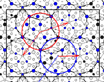
Figure 15: Test of the overlapping linkage in Fig. 4(a). Tile edges marked are 4Å long; heavy edges mark 13Å decagons(or 4Å-edge Star and Boat tiles that fill the space between 13Å Ds). Atom colors indicate species as in Fig. 2 Blue and red circles indicate Thin red arrows, fat red arrow, and blue arrow indicate hypothetical linkages of length $\tau^{3}a_{R}$, $1.176\tau^{2}a_{R}R$, and ${\sqrt{5}}\tau^{2}a_{R}$, respectively.

Now, the red circle in Fig. 15 shows an alternative place where the site list would have allowed a 13Å decagonto appear instead, overlapping as in Fig. 4 (a) with two other 13Å decagons; indeed, with the tiling shown, the site list in fact favors this alternative location. However, in a few tries of this sort, that cluster with the overlapping linkage never formed.

The blue circle in Fig. 15 shows another hypothetical cluster location forming a different linkage as indicated by the thick red arrow. It corresponds to edge sharing by the 2.45Å-edge decagons; in this case, the 13Å D  overlap forms a thin 4Å Hexagon.

Another test involved the simulations on the the 20$\times$38$\times$4 tiling mentioned at the end of Subsec. III.3. After short-time anneals on the small 2.45Å tiling, the configurations contained many Al₆TM₅ (ring 1) motifs, but the 13Å decagonswere imperfect and often interpenetrating, in contrast to the good ordering observed after similar annealing on the 32$\times$23 tiling. However, such configurations were $\sim 2$eV ($\sim 0.02$eV/atom) higher in energy than the $32\times 23$ tiling best energies. Furthermore, after 5 cpu hours of high-temperature ($T\sim 0.5$eV) annealing, these samples evolved to a proper configuration of 13Å decagons, which was in fact lower in energy than on the $32\times 23$ cells (with the same volume and atom content).

B.3 Rhombus cluster-cluster linkage?

Next we test the linkage shown in Fig. 4(b) In the 32$\times$23 cell, with content Al₁₄₅Co₄₁Ni₂₁ (hence density 0.0682 Å^-1), a followup fixed-site simulation was done, using the standard site list which avoids short Al-Co bonds. Three different 4Å-edge tilings were tried, each with four 13Å Dsspecified per cell. One of these tilings (Fig. 16 has four clusters at the vertices of a Fat rhombus. Its energy is roughly 2 meV/atom higher than the others. (We averaged this difference over the two cases where the 13Å D center orientations are all the same and where they are alternating). Since there is one 1.176$b^{\prime\prime}$ linkage in that cell, this amounts to a substantial cost of roughly 0.4eV for each such linkage.

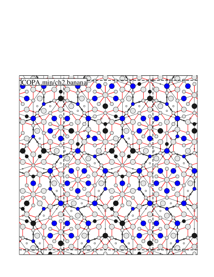
Figure 16: Test of the “rhombus diagonal” linkage in Fig. 4(b). The rhombus center is just below the cell’s upper-right corner (the fourth decagon, seen at lower-right corner; its copy by periodic boundary conditions is outside the upper frame.)

Appendix C Optimum configuration in channel: analytic calculation

This Appendix augments the mathematical details of the story in Sec. V.3, which are all consequences of the form of Al potential function $U(z)$ in a channel as written in Eq. (3). We assume the channel has three atoms, and derive the consequences.

C.1 Three-Al collective coordinate and local mirror layer

The main freedom of the three Al atoms in a channel is the collective $z$ coordinate ${\bar{z}}$. Let the respective Al positions as

$$z_{m}=(2c/3)m+{\bar{z}}+u_{m}$$ (7)

with $u_{m+3}\equiv u_{m}$, and constraining $\sum_{m=-1}^{+1}u_{m}=0$. [The mean displacement is accounted in the collective coordinate ${\bar{z}}$.] The total energy (per Al) is FN-omit2ndAl

$$E\equiv\frac{1}{3}\sum_{m=-1}^{+1}[U(z_{m})+V(z_{m+1}-z_{m}).$$ (8)

We want to find the best energy, given that ${\bar{z}}$ is fixed at a certain value. Taylor expanding (8 to second order in $\{u_{m}\}$ yields

$$E=E_{0}+\frac{1}{3}\sum_{m=-1}^{+1}[U^{\prime}({\bar{z}}+\frac{2c}{3}m)u_{m}+$$ (9)

$$U^{\prime\prime}({\bar{z}}+\frac{2c}{3}m)u_{m}^{2}+V^{\prime\prime}(\frac{2c}{3})(u_{m+1}-u_{m})^{2}$$

where $E_{0}\equiv U_{0}+V(2c/3)$. If we omit the $U_{c}$ term in (3), the minimum of the quadratic form (C.1) is FN-solve-Echannel

$$E({\bar{z}})=E_{0}-\frac{1}{6}\frac{B_{U}^{2}}{K_{V}^{2}-K_{U}^{2}}\left[K_{V}+K_{U}\cos\frac{12\pi}{c}{\bar{z}}\right],$$ (10)

where $K_{V}\equiv 3V^{\prime\prime}(2c/3)\;$ $K_{U}\equiv(4\pi/c)^{2}U_{c/2}$, and $B_{U}\equiv\sqrt{3/2}(4\pi/c)U_{c/2}$. The effective potential $E({\bar{z}})$ in general has a period $c/3$, one-third of the unit cell periodicity, since sliding the Al chain by $\pm 2c/3$ would move each Al atom to the old position of its neighbor, and additionally the potential is invariant under a shift $\pm c$. [The period in Eq. (10) is $c/6$, not $c/3$, since we assumed as a simplification that $U(z)$ has period $c/2$, not $c$.] The minimum configuration can be written ${\bar{z}}=0$ or $c/2$, with $u_{-1}=-u_{1}$ and $u_{0}=0$, so the channel has a local mirror layer at $z={\bar{z}}$.

Although the local minima of (3) as a function of the single-atom $z$ are quite strong, the effective potential $E({\bar{z}})$ is much flatter as a function of the collective coordinate, since the three atoms are constrained to sample different, counterbalanced parts of the potential. One can quantify “much flatter”, using the assertion above that Al-Al interactions are stronger (within a channel) than the Al potential due to Al-TM interactions. i.e. that $U^{\prime\prime}(2c/3)/V^{\prime\prime}(2c/3)\sim K_{U}/K_{V}\ll 1$. This implies via (10) that the ratio of the energy variations of the collective to those of the one-body potential is $\Delta E({\bar{z}})/\Delta U(z)\sim(K_{U}/K_{V})^{2}$. Thus, it is conceivable that the Al atoms in each vertical channel have, at moderate temperatures, considerable freedom to fluctuate (collectively) in the $z$ direction.

C.2 Further symmetry reduction by TM-rich layer

We now address the role of the $U_{c}$ term in eq. (3). It often happens that (in the language of the 4.0Å tiling) there are two tile edges forming a 72^∘ angle, with a Co column over each of the three vertices, and channels on both the mid-edges. (For example, this can involve ring 1 and ring 3 Co atoms in the 13Å D). From the viewpoint of one channel, one Co column is distant and breaks the $c/2$ periodicity: this is the justification of the last term in (3). To explain the sign of that term, note that if an Al in the channel is in the same layer as a distant Co, the separation is $R=3.80$Å, close to a local maximum of the Al-Co potential, whereas if Al is offset by one layer then $R=4.47$Å to the distant Co atoms, close to a local minimum (see Table 1).

Now consider the implication for the collective coordinate, when we include the $U_{c}$ term of (3). That will generate an additional contribution to $E({\bar{z}})$ of form $-\sigma{\rm const}\cos\frac{6\pi}{c}{\bar{z}}$. As it turns out, the sign of this term favors the mirror atom to sit in the same layer as the distant column of TM atoms (this is reversed from the layer preferred by the single-atom potential). Simulations show it is favorable for the atom occupancies to arrange themselves such that one layer of the two layers is richer in TM, which causes the puckering to develop such that this layer is a mirror layer globally. That is directly associated with the long-range order of decagon orientations (Sec. VI) and of puckering (VII.)

C.3 Transverse displacements in channels

In the above account, the displacements of Al atoms in channels to balance the “external” Al potential with Al-Al repulsions were represented as purely in the $z$ direction, only to allow a transparent analytic description. A more exact analysis would need to consider the transverse variation of the potential trough, for the Al-Al repulsion obviously should be based on the total Al-Al distance, and not just its $z$ component. In fact, the transverse undulation of the channel (bottom) line as a function of $z$ [see Fig. 11(a)], as well as the $xy$ deviations of the atoms from the channel line, may well make a contribution to the total $E({\bar{z}})$ comparable to the dependence in (10). For example, to make all three Al-Al separations be equal at $R=2.87$Å, the puckering displacement must be $(c-R)/2=0.645$Å, and the $xy$ difference between the puckered-layer site and the mirror-layer site should be $\sqrt{R^{2}-(c-R/2)^{2}}=0.90$Å. For comparison, the channel’s extremes are practically on ideal sites, separated in the $xy$ direction by $\tau^{-2}a_{0}\approx 0.94$Å. The actual $xy$ displacement would be only 2/3 that much if Al are assumed to stay on the bottom line, where the latter is approximated a “sawtooth” pattern of straight segments and the Al $z$ components are approximated as equally spaced.

Appendix D Labels of puckering patterns

In this appendix, we give detailed ways to label and enumerate possible configurations of a puckering unit (the short labels were explained in Sec. VII.3.1).

To exhaustively specify the puckering configuration around the center, we list the mirror-layer Al atoms, giving the angular placement $l$ of each [meaning angle $(2\pi/5)l$], and its puckering sense ($+$ if found in mirror layer 0, or $-$ if in mirror layer 2): The zero angle is defined as the shared 13Å D  edge (for type $A$ puckering unit) or the ray through the 13Å D  center (for any type $B$ puckering unit). An integer-plus-half angle is a “merged” channel site, as discussed in Sec. VII.2. The constraints on these sequences are (i) two atoms in the same layer must differ in angle by at least 1.5 steps; (ii) for every $l=0,...,4$ at least one atom must either have that $l$, or else have $l\pm 0.5$.

The short name of a $B$ pattern can have a parity superscript “$+$” or “$-$” added, meaning that the atoms at (or near) angles 1 and 4 (on the 13Å D  edges) have the same or opposite puckering sense, respectively: this indicates how the puckering sense propagates around the 13Å D. As we noted in Sec. VII.3.1, the $-$ parity is commonest, suggesting ${{\cal J}^{\rm puck}_{\alpha\beta}}$ is “antiferromagnetic” for second nearest neighbor channels around a puckering unit center. A straightforward explanation would be that the ideal sites of mirror-layer Al atoms, two angle steps apart, are separated by $2\sin(\pi/5)\tau^{-1}a_{0}\approx$ 2.88Å, which is close enough that the Al-Al repulsion is significant. In an “$A$” pattern, the parity is undefined, since it would be $+$ on one of the 13Å Ds  and is $-$ on the other one. (That follows since the mirror-layer Al atoms at angles 2 and 3, over the unshared 13Å D  edges meeting at the vertex, always have opposite puckering senses.)

Some common arrangements are listed in Table 8. The two standard kinds of “crooked cross” appear here as “$p4^{+}$” (one arm aligned radially and the other tangentially), or “$p4^{-}$” (arms about 45^∘ from the radial axis). (The $p4$ pattern in the “$A$” environment is a “crooked cross” which, when labeled as if on an unshared vertex, would be $p4^{+}$ from one cluster’s viewpoint and $p4^{-}$ from the other’s.) The common $A(p5)$ pattern could be described as another way to resolve the frustration of the puckering sense. As in Subsec. VII.2), imagine we alternate puckering senses ${\mu}_{\alpha}$ around the five channels, necessarily with one adjacent pair having the same sign. Instead of merging these atoms, keep all five and accomodate the steric constraint by displacing one of them by half an angle step.

Location	Short name	Long name
$A$	$p5$	$(0+,1-,2+,3-,4.5-)$
$A$	$u6$	$(0\pm,1.5\pm,3.5\pm)$
$B_{0}$	$p4^{-}$	$(1+,2-,3+,5-)$
$B_{0}$	$p5^{+}$	$(0+,1-,1.5+,2.5-,4-)$
$B_{1}$	$p4^{+}$	$(0+,1-,2.5+,4-)$
$B_{1}$	$p5^{+}$	$(0+,1-,2.5\pm,4-)$
$B_{1}$	$u6$	$(1\pm,2.5\pm,4\pm)$

Table 8: Common puckering patterns.

Appendix E 20Å decagon models?

In this appendix, we compare our results to three recent experiment-based structure models, all based on some sort of 20Å diameter decagon (the first two being similar to the Burkov cluster of Subsec. IV.6). We then report on a trial simulation of our own, using the methods of Sec. III but with an enriched site list for the lattice gas, from which a 20Å decagon packing emerges that is competitive in energy with the 13Å model developed in this paper.

E.1 Structure models based on PD4 approximant

After most of our work was completed, a tentative structure solution appeared for the approximant PD4 of the Co-rich phase oley06 with nominal composition Al_72.5Co₁₈Ni_9.5. The $c$ projection (see their Fig. 3) clearly shows an arrangement of decagonal clusters of diameter $20$Å (larger than the 13Å decagon  by exactly the factor $\tau$). This 20Å cluster appears practically the same as the Burkov cluster which – as we explained in Subsec. IV.6 – appears in our structure model. Namely, this decagon has rings 1,2, and 3 like our 13Å D  of Sec. III.2; their ring 3 Al show deviations into ring 2.5, similar to what occurs in our structures. In half of their clusters, ring 1 is missing a couple of Al atoms; these have more irregularity of their ring 2.5/3 Al atoms.

The big difference is that, in PD4, the 20Å decagons do not overlap; instead, they decorate a Fat rhombus with edge 10.4Å. Thus, the cluster-cluster linkages in this model are of length $\tau^{3}a_{0}=10.4$Å, for 20Å decagons sharing an edge, or $1.176\tau^{3}a_{0}=12.2$Å, for 20Å decagons related by the short diagonal of a Fat rhombus. It may also be noted that the cluster orientation pattern in PD4 is neither “ferromagnetic” nor “antiferromagnetic”; this would suggest that (in terms of Sec. VI the 12.2Å linkage induces an “antiferromagnetic” interaction.

Although the “Star cluster” motifs no longer sit at vertices of this 19.7Å edge network, that atom cluster is still in evidence. The difference is that in the PD4 structure, every 13Å D  is encircled by ten such Star clusters, whereas this number was smaller in our model of Fig. 7. The PD4 atomic structure, like the rigid-site-list models of Sec. IV, can be decomposed into a DHBS (Decagon-Hexagon-Boat-Star) tiling with edge $a_{0}=2.45$Å.

In fact, a decagonal model based on PD4 is a concrete example of the structure models intermediate between the “basic Ni” decoration of Ref. alnico01, and the decoration of our Sec. IV. Such a hybrid model would have 8Å decagons, which are absent in the former decoration, but have a larger proportion of 2.45Å HBS tiles than in the latter decoration. (In particular, every edge of the 20Å decagon is the centerline of a 2.45Å Hexagon, decorated typically by a Ni-Ni pair.) We expected such an intermediate model to be favored at an intermediate composition such as Al₇₀Co₁₅Ni₁₅, but the energy differences are quite small, so it may well be competitive at the compositions the present paper focuses on.

E.2 Structure model from Al₇₁Ni₂₂Co₇ approximant

Another decagonal approximant was discovered with composition Al₇₁Ni₂₂Co₇, close to the “basic Ni” phase, and a structure model developed based on electron diffraction and Z-contrast imaging abe06-ICQ9 . This model consists of edge-sharing 20Å decagons of the kind we have been describing. They have Al₆TM₅ cores, alternating in orientation (the cluster network happens to be bipartite). There are no ring 2.5 Al; about half the edges of the 13Å decagons  (contained in the 20Å one) have two ring 3 Al, the other half of the edges have only one ring 3 Al. The edges of the 20Å decagons, without exception, have two TM atoms.

A good interpretation of the cluster network in Ref. abe06-ICQ9, is that the 20Å (edge 6.4Å) decagons occupy the Large sites of a Binary tiling with edge 16.8Å, while pentagonal bipyramids (PBs) occupy the Small sites. The vertices of the 20Å decagons, as in the PD4 model, are occupied by motifs like the Star cluster. Such Star clusters  also occur between pairs of adjacent PBs. There, they define additional tile vertices which divide the area between the 20Å decagons into Hexagons, Boats, and Stars with edge 6.5Å.

E.3 Structure model based on W(AlCoNi) approximant

Deloudi et al del06 have presented a structure model (formulated in a 5D-cut framework) for the same Co-rich composition we address here. They formulate a 20Å pentagonal cluster, which is built around the W-phased pentagon cluster; these can overlap in various ways. The Al/TM assignments in the model are based entirely on those reported in Sugiyama’s $W$(AlCoNi) refinement Su02 .

Examination of their Fig. 1 reveals the relation between their cluster and our 13Å decagon  motif. Take each vertex of their 20Å  decagon that is not a vertex of the inscribed large pentagon, and draw an arc around it through the adjacent decagon vertices (which are vertices of the inscribed pentagon); this arc encloses 3/10 of a 13Å decagon. Their model, being based on a stacking period $2c\approx 8$Å, accomodates not only the pentagonal bipyramid (PB), but also the puckering of the Al atoms we called ring 2.5/ring 3 (or better, channel atoms) along the arcs just mentioned.

In Fig. 3(a) of Ref. del06, it can be seen that 13Å decagons, although not recognized at all in their formulation, are naturally generated in the interstices between the large pentagons. The overall pattern could be decribed as a packing of edge-sharing 32Å super-decagons (inflated by one factor of $\tau$), with PBs  placed on the super-decagon centers and odd vertices, and 13Å decagons  on the super-decagon even vertices. (It is not surprising to find descriptions on different length scales: their model, being essentially a decoration of the quasiperiodic Penrose tiling, acquires its inflation symmetry.)

We question whether the details of this model are good energetically. Our study suggests that good models are built by combinations of the 8Å decagon (the central part of the 13Å decagon), of 2.45Å edge HBS tiles, plus the PB. To the extent that this model appears to have incomplete fragments of the 8Å decagon, we suspect it will have an increased energy. It is conceivable that only Al atoms are wrong, and the TM atoms are correctly placed, which would still give good agreement with electron micrographs of all kinds.

The 13Å decagons show up prominently in the experimental HAADF-STEM image of Ref. del06, (their Fig. 3(b)) as white pentagons, all oriented the same way. These are not as frequent as they would be in the decoration of our Fig. 7, suggesting that our model is not correct for that composition.

E.4 Preliminary simulations with 20Å clusters

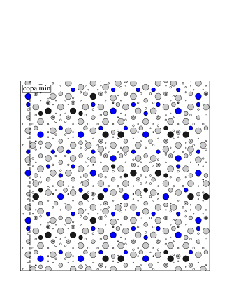
Figure 17: Fixed-site simulation in which 20Å decagons emerge.

Fig. 17 shows an exploratory fixed-site lattice-gas simulation on a 4Å tiling in the 32$\times$23 cell, similar to Sec. III.5, but with a richer set of candidate sites decorating the tiles, and a much longer annealing time. Two 20Å decagons are seen in this configuration, in place of the four 13Å decagons that typically emerged in our main simulations. The atomic structure is quite similar to those described above; a minor difference is that every edge of the 13Å decagon  has exactly one ring 3 Al, and their placement alternates perfectly. (That alternation was necessarily disrupted in our model of Sec. IV, wherever the 13Å D’s shared edges.) Also, the edges of the 20Å decagon are not only Ni-Ni, but often Al-Co or Ni-Co in Fig. 17. It would take much more work to settle the optimum decoration of these sites, and the optimum atom content for a decoration based on such configurations.

The 20Å based configuration of Fig. 17 is lower in energy by 1.8 meV/atom as compared to the best result of the 13Å sort produced by our 4Å simulations, if ideal-site configurations are compared. However, after the RMR protocol in an 8Å cell (see Sec. V), the 20Å type structure was slightly higher in energy, by 0.6 meV/atom, than the 13Å type structure. (The latter probably contains more Al channels, and thus offers more opportunity to reduce energy by puckering.)

E.5 Ways our approach can mislead

FROM email: mvic-colong-disc.out0622)

Overall, it is our impression that – despite the deficiencies (known and still unknown) in our potentials, the biggest problem for achieving a correct structure is the search pathway to find it. On the one hand, we think our method has been remarkably successful at predicting characteristic features such as the appearance of the 13Å decagonin Co-rich compositions.

On the other hand, we have recounted four ways in which our procedure misled us: (i) the fixed site list (ii) the 8 Å periodicity (iii) the possibility of a larger cluster than 13Å D(iv) the cluster orientation order

A separate note is that our calculations are good only to predict stability between similar decagonal approximant structures. Many deficiencies of our potentials – the dependence on electron density (and hence on composition, in principle); inaccuracies in the nearest-neighbor TM-TM and TM-Al potential wells; cutoffs at some interaction radius; omission of three- or four-body terms; and poor handling of vacancies – will tend to cancel, in such a comparison. But any phase may, of course, be preempted by a coexistence of two dissimilar phases that happens to have a slightly lower energy; our pair potentials are more likely to give a wrong answer in this situation. To construct a global phase diagram, it is necessary to follow up the kind of search described in this paper, by ab-initio total energy calculations, with an attempt to imagine all possible competing phases and include them in this database. Since it would be prohibitive to try out a large set of candidate structures with the ab-initio codes, the present sort of study is a prerequisite to the phase-diagram studies.

References

- (1) Permanent address, Institute of Physics, Slovak Academy of Sciences, 84228 Bratislava, Slovakia.
- (2) S. Ritsch, C. Beeli, H. U. Nissen, T. Gödecke, M. Scheffer, and R. Lück, Phil. Mag. Lett., 74, (1996) 99-106
- (3) S. Ritsch, C. Beeli, H. U. Nissen, T. Gödecke, M. Scheffer, and R. Lück, Phil. Mag. Lett. 78, 67-76 (1998). Philos. Mag. Lett. 78, 67 (1998)
- (4) H. Takakura, A. Yamamoto, and A. P. Tsai, Acta Crystallogr. A 57: 576 (2001); A. Cervellino, T. Haibach, and W. Steurer, Acta Crystallogr. B 58, 8 (2002).
- (5) B. Grushko, D. Holland-Moritz, and K. Bickmann, J. Alloys Comp. 236, 243 (1996) Decagonal quasicrystals in Al-Co and ternary
- (6) X. Z. Li, R. C. Yu, K. H. Kuo, and K. Hiraga, Phil. Mag. Lett. 73, 255 (1996).
- (7) S. Ritsch, C. Beeli, and H.-U. Nissen, Phil. Mag. Lett. 74, 203 (1996).
- (8) S. Ritsch, H.-U. Nissen, and C. Beeli, Phys. Rev. Lett. 76, 2507 (1996).
- (9) S. Ritsch, O. Radulescu, C. Beeli, D. H. Warrington, R. Lück, and K. Hiraga, Phil. Mag. Lett. 80, 107 (2000).
- (10) K. Sugiyama, S. Nishimura, and K. Hiraga, J. Alloy Comp. 342, 65 (2002).
- (11) W. Steurer, personal communication.
- (12) F. Frey, E. Weidner, K. Hradil, M. De Boissieu, R. Currat, K. Shibata, A. P. Tsai, and T. J. Sato, Phil. Mag. A. 80, 2375-91 (2000)
- (13) F. Frey, Mater. Sci. Eng. A 294, 178-85 (2000).
- (14) M. Mihalkovič, I. Al-Lehyani, E. Cockayne, C. L. Henley, N. Moghadam, J. A. Moriarty, Y. Wang, and M. Widom, Phys. Rev. B 65, 104205 (2002).
- (15) C. L. Henley, M. Mihalkovič, and M. Widom, J. All. Compd. 342 (1-2): 221 (2002).
- (16) N. Gu, M. Mihalkovič, and C. L. Henley, unpublished (submitted to Phil. Mag. Lett.).
- (17) N. Gu, C. L. Henley, and M. Mihalkovič, Phil. Mag. 86, 593 (2006).
- (18) M. Mihalkovič, C. L. Henley, and M. Widom, J. Non-Cyst. Sol. 334: 177 (2004).
- (19) J. Roth and C. L. Henley, Philos. Mag. A, Vol 75 (No 3), 861 (1997).
- (20) J. A. Moriarty and M. Widom, Phys. Rev. B 56, 7905 (1997).
- (21) I. Al-Lehyani, M. Widom, Y. Wang, N. Moghadam, G.M. Stocks and J.A. Moriarty, Phys. Rev. B 64, 075109 (2001).
- (22) The GPT potentials, although systematically founded, appear to underrepresent the real interactions in (AlNiCo) by a factor of up to 2, as inferred from comparisons to experimental phonon spectra (M. Mihalkovic, unpublished).
- (23) M. Widom and J.A. Moriarty, Phys. Rev. B 58, 8967 (1998); M. Widom, I. Al-Lehyani and J.A. Moriarty, Phys. Rev. B 62, 3648 (2000).
- (24) M. Widom and E. Cockayne, Physica A 232, 713 (1996).
- (25) S. Katrych, M. Mihalkovič, V. Gramlich, M. Widom and W. Steurer, Phil. Mag. A 86, 451 (2006).
- (26) M. Mihalkovič and M. Widom, Phil. Mag. A 86, 557 (2006).
- (27) In the initial stage Monte Carlo simulations, a better procedure would have been to use (at least) two densities, bracketing the physical one, as elaborated in Sec. IX.1.
- (28) H.-C. Jeong and P. J. Steinhardt, Phys. Rev. Lett. 73, 1943 (1994).
- (29) C. L. Henley, p. 27 in Quasicrystals, ed. S. Takeuchi and T. Fujiwara (World Scientific, Singapore, 1998).
- (30) In some runs, samples were only cooled to , corresponding to 3000 K (which would be well above the melting point, but the constraint of a discrete site list makes a large difference) But low energy structures obtained at these high temperatures were quite similar in configuration to those obtained from low temperatures, in that the decagonal rings were pretty well bound together: the structures that are favorable are, in general, the same as those favorable at .
- (31) The initial stage simulations in Ref. alnico01, for the “basic Ni” phase used a smaller unit cell that was probably too small. If used in the “basic Co” case, it would have hindered us from discovering the right motifs.
- (32) E. Cockayne and M. Widom, Philos. Mag. A 77, 593 (1998); E. Cockayne and M. Widom, Phys. Rev. Lett. 81, 598 (1998).
- (33) R. Penrose, Math. Intelligencer 2, 32 (1979)
- (34) C. L. Henley, ‘Random tiling models,’ p. 429 in Quasicrystals: The State of the Art, ed. P. J. Steinhardt and D. P. DiVincenzo, (World Scientific, 1991).
- (35) C. L. Henley, Phys. Rev. B34, 797 (1986).
- (36) S. Hiramatsu and Y. Ishii, J. Phys. Soc. Jpn. 2006 (submitted).
- (37) M. Mihalkovič, W.-J. Zhu, C. L. Henley, and R. Phillips, Phys. Rev. B 53, 9021 (1996).
- (38) F. Lançon, L. Billard, and P. Chaudhari, Europhys. Lett. 2, 625 (1986); M. Widom, K. J. Strandburg, and R. H. Swendsen, Phys. Rev. Lett. 58, 706 (1987)
- (39) C. L. Henley, J. Non-Cryst. Solids 153&154, 172-176 (1993).
- (40) I. Al-Lehyani and M. Widom, Phys. Rev. B 67, 014204 (2003).
- (41) The augmented site list used in Sec. E.4 does produce exactly the same site list, no matter how the 4Å rhombi are packed between 13Å star decagons.
- (42) The temperature is lower because these simulations have fewer degrees of freedom than the Å simulations.
- (43) C. L. Henley, Phil. Mag. A 86, 1123 (2006); C. L. Henley, M. de Boissieu, and W. Steurer (eds.), Phil. Mag. A 86, 1131 (2006).
- (44) K. Saitoh, M. Tanaka, A. P. Tsai, and C. J. Rossouw, J. Phys. Soc. Jpn. 69, 2379 (2000).
- (45) B. Grushko and M. Döblinger, Z. Kristallogr. 219, 447 (2004).
- (46) A. Yamamoto, H. Takakura, and E. Abe, Phys. Rev. B72, 144202 (2005)
- (47) S. E. Burkov, Phys. Rev. Lett. 67, 614 (1991).
- (48) W. Steurer and K. H. Kuo, Acta Crystallogr. B 46, 703 (1990)
- (49) K. Hiraga, W. Sun, and F. J. Lincoln, Jap. J. Appl. Phys. 30, L302 (1991).
- (50) S. Deloudi, M. Kobas, and W. Steurer, Phil. Mag. 86, 581 (2006)
- (51) More generally, a potential map may defined whenever a securely occupied subset of sites can be identified. Its efficacy depends on how nicely the problem of placing the remaining atoms factorizes into independent problems. In the present case, we might (after filling the deep wells with Al) define a second potential map, which would be more realistic since the undetermined Al atoms obviously do interact with the well-determined ones. However, the images of such a potential function (which is dominated by forbidden zones where the atoms have been filled in) are harder to relate to the atomic structures, and we did not use them in the present work.
- (52) Observe how the ring-1 Al well extends in the plane outward from the cluster center (in the Star clusteras well as 13Å D). helping explain shifts in the position under relaxation (subsec. V.1.1), and predicting an anisotropic Debye-Waller factor in diffraction experiments owing to fluctuations in that well.
- (53) If we simply take the idealized model of Fig. 7, and rotate every alternate 13Å D core by the 10-fold screw axis without any other modification, the energy increases by by 1 eV per cluster. This confirms how the ring 3 and Star cluster atoms adapt to various 13Å D orientations so as to make them nearly degenerate.
- (54) Note that is not the same as the variable that was defined in Sec. V.3 and used in Appendix C. In fact, the are well-defined only if certain layers (which we called 0 and 2) are mirror layers globally, and that happens only when takes the same value everywhere. In terms of the collective coordinate defined in eq. (7) to parametrize the sliding of three Al atoms in a channel, we could say , whereas (assuming a first symmetry-breaking ) .
- (55) F. Frey, Mater. Sci. Eng. A 294, 178 (2000).
- (56) S. Katrych and W. Steurer, Z. Kristallogr. 219, 806 (2004) .
- (57) B. Grushko, D. Hollard-Moritz, R. Wittmann, and G. Wilde, J. All. Comp. 280, 215 (1998).
- (58) L.-H.Tang and M. V. Jarić, PRB circa 1989, four-level (random) tiling.
- (59) The ‘DecaDeco’ package is still under development. A version of the code and its draft documentation may be obtained from Marek Mihalkovič.
- (60) In the simulations reported here, runs were performed as a series of repeated cooling cycles. Each succeeding cycle started from the last configuration of the previous cycle, at a very high temperature, so that we didn’t need to re-initialize random seed. Eventual variant runs were performed with different run parameters, or started from different seed configuration.
- (61) P. Villars, Pearson’s Handbook of crystallographic data for intermetallic phases (ASTM International, Materials Park, OH, 1991).
- (62) has eV variations between channels that do not affect this discussion.
- (63) Apart from the hard core, is so weak that we are fully justified in omitting from Eq. 8.
- (64) This solution took many steps: to manifest the symmetres was helpful to work using the basis vectors and for the subspace of allowed
- (65) A. Redfield and A. Zangwill, c. 1990, rationalizing Mackay Icosahedron in alpha-AlMnSi.
- (66) P. Oleynikov, I. Demchenko, J. Christensen, S. Hovmöller, T. Yokosawa, M. Döblinger, B. Grushko, and X. D. Zou, Phil. Mag. 86, 457 (2006). Their figure lacks information( which might reveal puckering).
- (67) E. Abe and A. Yamamoto, unpublished.