Three-body recombination of ultracold Bose gases using the truncated Wigner method

Abstract

We apply the truncated Wigner method to the process of three-body recombination in ultracold Bose gases. We find that within the validity regime of the Wigner truncation for two-body scattering, three-body recombination can be treated using a set of coupled stochastic differential equations that include diffusion terms, and can be simulated using known numerical methods. As an example we investigate the behaviour of a simple homogeneous Bose gas.

I Introduction

The dominant loss process affecting ultracold gaseous alkali metal systems is inelastic three-body recombination Moerdijk1996a ; Wieman1997a ; Dalibard1999a ; Esry1999a , a process characterised by collisional events involving three atoms leading to the creation of a single two-atom molecule (a dimer). The binding energy released by the molecule formation is retained by the particles as kinetic energy. Typically this results in the loss of all three atoms from the system as the molecule is not trapped by any applied external potential and the energy of the free atom is high enough to overcome any confinement barrier. Indeed it is this process that limits the lifetime of experimentally produced alkali metal Bose-Einstein condensates, due to the large increase in density once the temperature is lowered past the critical point Ketterle1995a .

In a previous paper Norrie2005b we presented a comprehensive treatment of the truncated Wigner approach for ultracold Bose gases including elastic two-body interactions. In this paper we extend that treatment to include three-body recombination events, which modifies the ensemble differential equations describing the evolution of a single realisation of the field. These modified differential equations are explicitly stochastic, including dynamic noise sources arising from the action of three-body recombination on the virtual particle background field.

To provide a demonstration of our extended formalism we examine the evolution of a simple homogeneous system, starting from a zero-temperature state where the particle population is initially confined to a single (condensate) mode.

I.1 Three-body recombination in ultracold gases

Assuming that three-body recombination is the only particle loss mechanism affecting the system, it can be shown that the rate of change of total particle number is Wieman1997a

$$\frac{dN\left(t\right)}{dt}=-3K_{3}\int d{\bf x}\,g^{\left(3\right)}\left({\bf x},t\right)n\left({\bf x},t\right)^{3},$$ (1)

where $n\left({\bf x},t\right)$ is the total number density of atoms and $K_{3}$ is the three-body recombination event rate constant. We have assumed that all the particles involved in the recombination process are lost from the system, hence the prefactor of 3 in Eq. (1), which describes the number of particles lost from the system. The third-order normalised equiposition correlation function $g^{\left(3\right)}\left({\bf x},t\right)$ measures the statistics of the field, being unity for a fully coherent system, i.e. a zero-temperature condensate, and $3!=6$ for a purely thermal system. The factor of 6 increase in the loss rate of thermal over coherent systems for similar densities has been observed experimentally Wieman1997a .

II Truncated Wigner treatment

II.1 The restricted field

As in our previous work Norrie2005b , we describe the many-body system of identical bosons using the Schrödinger picture bosonic field operator

$$\hat{\Psi}\left({\bf x}\right)=\sum_{j}\psi_{j}\left({\bf x}\right)\hat{a}_{j}.$$ (2)

Here the mode operators $\hat{a}_{j}$ annihilate a single boson from the $j$th mode, and obey the commutation relations

$$\left[\hat{a}_{i},\hat{a}_{j}\right]=\left[\hat{a}_{i}^{\dagger},\hat{a}_{j}^{\dagger}\right]=0,\hskip 14.22636pt\left[\hat{a}_{i},\hat{a}_{j}^{\dagger}\right]=\delta_{i,j},$$ (3)

while the coordinate space functions $\psi_{j}\left({\bf x}\right)$ form an infinite orthonormal basis set where

$$\left[-\frac{\hbar^{2}\nabla^{2}}{2m}+U_{\rm ext}\left({\bf x}\right)\right]\psi_{j}\left({\bf x}\right)=\hbar\omega_{j}\psi_{j}\left({\bf x}\right),$$ (4)

where $U_{\rm ext}\left({\bf x}\right)$ is the applied external potential.

We now divide mode space into two subspaces, a low-energy space ($L$) consisting of all those modes whose eigenenergies are less than the boundary energy $\varepsilon_{\rm cut}$, and a high-energy space ($H$) that includes all remaining modes. For this work our interest lies with the dynamics of the low-energy subspace. Using these subspaces we define the field operators

$$\hat{\Psi}_{\mathcal{P}}\left({\bf x}\right) \equiv \sum_{j\in L}\psi_{j}\left({\bf x}\right)\hat{a}_{j}$$ (5a)

$$\hat{\Psi}_{\mathcal{Q}}\left({\bf x}\right) \equiv \sum_{j\in H}\psi_{j}\left({\bf x}\right)\hat{a}_{j},$$ (5b)

Of most importance for this paper is the low-energy restricted basis field operator $\hat{\Psi}_{\mathcal{P}}\left({\bf x}\right)$, which can be obtained from the total field operator

$$\hat{\Psi}\left({\bf x}\right)\equiv\sum_{j\in L,H}\psi_{j}\left({\bf x}\right)\hat{a}_{j},$$ (6)

using the projector

$$\mathcal{P}\equiv\sum_{j\in L}\left|j\right\rangle\left\langle j\right|$$ (7)

as $\hat{\Psi}_{\mathcal{P}}\left({\bf x}\right)=\mathcal{P}\left[\hat{\Psi}\left({\bf x}\right)\right]$. The restricted basis field operator obeys the commutation relations

$$\left[\hat{\Psi}_{\mathcal{P}}\left({\bf x}\right),\hat{\Psi}_{\mathcal{P}}\left({\bf x}^{\prime}\right)\right] = \left[\hat{\Psi}_{\mathcal{P}}^{\dagger}\left({\bf x}\right),\hat{\Psi}_{\mathcal{P}}^{\dagger}\left({\bf x}^{\prime}\right)\right]=0$$

$$\left[\hat{\Psi}_{\mathcal{P}}\left({\bf x}\right),\hat{\Psi}_{\mathcal{P}}^{\dagger}\left({\bf x}^{\prime}\right)\right] = \delta_{\mathcal{P}}\left({\bf x},{\bf x}^{\prime}\right),\hskip 28.45274pt$$ (8)

where the restricted delta function is defined by

$$\delta_{\mathcal{P}}\left({\bf x},{\bf x}^{\prime}\right)\equiv\sum_{j\in L}\psi_{j}^{*}\left({\bf x}^{\prime}\right)\psi_{j}\left({\bf x}\right).$$ (9)

The conjugate projector $\mathcal{Q}$ can be obtained using the complementarity relation $\mathcal{P}+\mathcal{Q}=1$.

II.2 Master equation

Our previous paper Norrie2005b assumed that only two atoms participate in any single scattering event. In this way the particle interactions are described using a simple $s$-wave contact potential as an approximation to the full two-body T-matrix. Obviously such a description does not include three-body scattering events. Full theoretical treatments of three-body scattering including all possible collisional channels are extremely complicated, and we do not attempt such an approach here. Instead we adopt a quantum-optical approach, starting from a phenomenologically appropriate Hamiltonian including inelastic three-body recombination events, to which we apply the truncated Wigner method.

We assume that within the dilute limit the characteristic range of the three-body recombination potential $U_{\rm TBR}\left({\bf x}_{1},{\bf x}_{2},{\bf x}_{3}\right)$ is much smaller than the average interparticle spacing. Thus, following thematically the approach for pairwise scattering, we replace this scattering potential by an effective zero-range three-body scattering T-operator, whose interaction strength is essentially a free parameter that will be chosen to satisfy experimentally observed loss rates. Within this approach then, in order to include the effects of three-body recombination the Schrödinger picture effective Hamiltonian is modified to include the term Jack2002a

$$\hat{H}_{\rm eff}^{\rm\left(TBR\right)}=\kappa_{\rm TBR}\int d{\bf x}\left[\hat{\Psi}_{\mathcal{Q}}^{\dagger}\left({\bf x}\right)\hat{\Xi}^{\dagger}\left({\bf x}\right)\left(\hat{\Psi}_{\mathcal{P}}\left({\bf x}\right)\right)^{3}+\left(\hat{\Psi}_{\mathcal{P}}^{\dagger}\left({\bf x}\right)\right)^{3}\hat{\Psi}_{\mathcal{Q}}\left({\bf x}\right)\hat{\Xi}\left({\bf x}\right)\right].$$ (10)

where the molecule field operator $\hat{\Xi}\left({\bf x}\right)$ annihilates a dimer from the field and $\kappa_{\rm TBR}$ is a measure of the energy associated with the three-body process. We have assumed in formulating Eq. (10) that the binding energy associated with the molecule formation is large enough that the unpaired atom generated by a recombination event is created within the high-energy subspace $H$, rather than the low-energy (system) subspace $L$, and is described by the high-energy field operator $\hat{\Psi}_{\mathcal{Q}}\left({\bf x}\right)$.

Jack Jack2002a has considered this partial Hamiltonian, and has shown that by eliminating both the molecular and high-energy atomic fields from the evolution using a standard interaction picture approach for initially uncoupled fields Walls1994a , one obtains the master equation term

$$\frac{d\rho\left(t\right)}{dt}^{\rm\left(TBR\right)} = \frac{\gamma}{6}\int d{\bf x}\left[2\left(\hat{\Psi}_{\mathcal{P}}\left({\bf x}\right)\right)^{3}\rho\left(t\right)\left(\hat{\Psi}_{\mathcal{P}}^{\dagger}\left({\bf x}\right)\right)^{3}-\left(\hat{\Psi}_{\mathcal{P}}^{\dagger}\left({\bf x}\right)\right)^{3}\left(\hat{\Psi}_{\mathcal{P}}\left({\bf x}\right)\right)^{3}\rho\left(t\right)\right.$$ (11)

$$\left.\mbox{}-\rho\left(t\right)\left(\hat{\Psi}_{\mathcal{P}}^{\dagger}\left({\bf x}\right)\right)^{3}\left(\hat{\Psi}_{\mathcal{P}}\left({\bf x}\right)\right)^{3}\right],$$

for the low-energy atomic subspace (system) density operator $\rho\left(t\right)$. The quantity $\gamma$ governs the rate of recombination events, and its relationship to $K_{3}$ we consider later. In arriving at this master equation term it has been assumed that the output products of the recombination events immediately exit the coordinate space region containing the system, such that they play no further role in the evolution. To describe the full master equation for the system density operator one combines Eq. (11) with the von Neumann equation calculated in Norrie2005b .

II.3 Functional Wigner function correspondences

The master equation term given by Eq. (11) can be used to calculate the evolution of the corresponding multimode Wigner function $W\left(\left\{\alpha_{j},\alpha_{j}^{*}\right\},t\right)$ using appropriate operator correspondences Gardiner2000a . However, rather than using the mode operator correspondences that were used in Norrie2005b , here we perform this step using functional operator correspondences.

We define, similar to the restricted basis field operator $\hat{\Psi}_{\mathcal{P}}\left({\bf x}\right)$, the restricted basis wavefunctions

$$\Psi_{\mathcal{P}}\left({\bf x}\right) \equiv \sum_{j\in L}\psi_{j}\left({\bf x}\right)\alpha_{j}$$ (12a)

$$\Psi^{*}_{\mathcal{P}}\left({\bf x}\right) \equiv \sum_{j\in L}\psi_{j}^{*}\left({\bf x}\right)\alpha_{j}^{*}$$ (12b)

and the related functional derivatives

$$\frac{\delta}{\delta\Psi_{\mathcal{P}}\left({\bf x}\right)} \equiv \sum_{j\in L}\psi_{j}^{*}\left({\bf x}\right)\frac{\partial}{\partial\alpha_{j}}$$ (13a)

$$\frac{\delta}{\delta\Psi^{*}_{\mathcal{P}}\left({\bf x}\right)} \equiv \sum_{j\in L}\psi_{j}\left({\bf x}\right)\frac{\partial}{\partial\alpha_{j}^{*}}.$$ (13b)

Using these definitions together with the Wigner function mode operator correpondences Gardiner2000a , we find that the actions of the restricted basis field operator on the system density operator $\rho\left(t\right)$ can be expressed as actions on the corresponding Wigner function using

$$\hat{\Psi}_{\mathcal{P}}\left({\bf x}\right)\rho\left(t\right) \leftrightarrow \left(\Psi_{\mathcal{P}}\left({\bf x}\right)+\frac{1}{2}\frac{\delta}{\delta\Psi^{*}_{\mathcal{P}}\left({\bf x}\right)}\right)W\left(t\right)$$ (14a)

$$\hat{\Psi}^{\dagger}_{\mathcal{P}}\left({\bf x}\right)\rho\left(t\right) \leftrightarrow \left(\Psi^{*}_{\mathcal{P}}\left({\bf x}\right)-\frac{1}{2}\frac{\delta}{\delta\Psi_{\mathcal{P}}\left({\bf x}\right)}\right)W\left(t\right)$$ (14b)

$$\rho\left(t\right)\hat{\Psi}_{\mathcal{P}}\left({\bf x}\right) \leftrightarrow \left(\Psi_{\mathcal{P}}\left({\bf x}\right)-\frac{1}{2}\frac{\delta}{\delta\Psi^{*}_{\mathcal{P}}\left({\bf x}\right)}\right)W\left(t\right)$$ (14c)

$$\rho\left(t\right)\hat{\Psi}^{\dagger}_{\mathcal{P}}\left({\bf x}\right) \leftrightarrow \left(\Psi^{*}_{\mathcal{P}}\left({\bf x}\right)+\frac{1}{2}\frac{\delta}{\delta\Psi_{\mathcal{P}}\left({\bf x}\right)}\right)W\left(t\right).$$ (14d)

Such functional Wigner function operator correspondences have been previously used by Steel et al. Steel1998a .

II.4 Wigner function evolution

Applying the functional Wigner function operator correspondences, Eq. (14), to the master equation term describing three-body recombination, Eq. (11), we obtain, after some manipulation, the Wigner function evolution term

$$\frac{\partial W}{\partial t}^{\rm\left(TBR\right)} = \frac{\gamma}{6}\int d{\bf x}\left[\left(\frac{\delta}{\delta\Psi_{\mathcal{P}}}\Psi_{\mathcal{P}}+\frac{\delta}{\delta\Psi_{\mathcal{P}}^{*}}\Psi_{\mathcal{P}}^{*}\right)\right.\left(3\left|\Psi_{\mathcal{P}}\right|^{4}-9\left|\Psi_{\mathcal{P}}\right|^{2}\delta_{\mathcal{P}}\left({\bf x},{\bf x}\right)+\frac{9}{2}\delta_{\mathcal{P}}\left({\bf x},{\bf x}\right)^{2}\right)$$ (15)

$$\mbox{}+\frac{\delta^{2}}{\delta\Psi_{\mathcal{P}}\delta\Psi_{\mathcal{P}}^{*}}\left(9\left|\Psi_{\mathcal{P}}\right|^{4}-18\left|\Psi_{\mathcal{P}}\right|^{2}\delta_{\mathcal{P}}\left({\bf x},{\bf x}\right)+\frac{9}{2}\delta_{\mathcal{P}}\left({\bf x},{\bf x}\right)^{2}\right)+\frac{1}{4}\left(\frac{\delta^{3}}{\delta\Psi_{\mathcal{P}}^{3}}\Psi_{\mathcal{P}}^{3}+\frac{\delta^{3}}{\delta\Psi_{\mathcal{P}}^{*3}}\Psi_{\mathcal{P}}^{*3}\right)$$

$$\mbox{}+\frac{9}{4}\left(\frac{\delta^{3}}{\delta\Psi_{\mathcal{P}}^{2}\delta\Psi_{\mathcal{P}}^{*}}\Psi_{\mathcal{P}}+\frac{\delta^{3}}{\delta\Psi_{\mathcal{P}}\delta\Psi_{\mathcal{P}}^{*2}}\Psi_{\mathcal{P}}^{*}\right)\left(\left|\Psi_{\mathcal{P}}\right|^{2}-\delta_{\mathcal{P}}\left({\bf x},{\bf x}\right)\right)+\frac{3}{4}\left(\frac{\delta^{4}}{\delta\Psi_{\mathcal{P}}^{3}\delta\Psi_{\mathcal{P}}^{*}}\Psi_{\mathcal{P}}^{2}+\frac{\delta^{4}}{\delta\Psi_{\mathcal{P}}\delta\Psi_{\mathcal{P}}^{*3}}\Psi_{\mathcal{P}}^{*2}\right)$$

$$\left.\mbox{}+\frac{3}{16}\left(\frac{\delta^{5}}{\delta\Psi_{\mathcal{P}}^{3}\delta\Psi_{\mathcal{P}}^{*2}}\Psi_{\mathcal{P}}+\frac{\delta^{5}}{\delta\Psi_{\mathcal{P}}^{2}\delta\Psi_{\mathcal{P}}^{*3}}\Psi_{\mathcal{P}}^{*}\right)+\frac{1}{16}\frac{\delta^{6}}{\delta\Psi_{\mathcal{P}}^{3}\delta\Psi_{\mathcal{P}}^{*3}}\right]W.$$

Eq. (15) is a rather complex equation of motion, including derivative terms up to sixth order. However, we can only write differential equations describing the evolution of a single ensemble member for Wigner function evolutions containing derivative terms up to second order. Thus to proceed we must truncate the higher order terms in Eq. (15), a process that is also required for the pairwise scattering Norrie2005b .

II.4.1 Wigner truncation

To justify the truncation of the higher order terms in the Wigner function evolution, we follow a similar method to that given in Norrie2005b . Let us assume that at some time $\tau$ the Wigner function of the (low-energy) system has the factorisable form

$$W\left(\left\{\alpha_{j},\alpha_{j}^{*}\right\},\tau\right)=\prod_{j\in L}\frac{\Gamma_{j}}{\pi}\exp\left[-\Gamma_{j}\left|\alpha_{j}-\alpha_{j_{0}}\right|^{2}\right].$$ (16)

Here $\alpha_{j_{0}}\equiv\left\langle\hat{a}_{j}\right\rangle$ is the expectation value amplitude of the $j$th mode, and $\Gamma_{j}$ is proportional to the inverse width of the Wigner function for that mode. This type of function describes both coherent (where $\Gamma_{j}=2$) and thermally distributed modes, but does not describe number states or other more exotic states. The factorisability of this Wigner function indicates that number fluctuations between disparate modes are uncorrelated.

Evaluating the Wigner function evolution given by Eq. (15) using the Wigner function given by Eq. (16) returns a rather complicated expression, which we give in full in the appendix, Eq. (44). Essentially we find that for increasing order in $\delta/\delta\Psi_{\mathcal{P}}$, the leading order term in $\left|\Psi_{\mathcal{P}}\right|$ decreases. In performing the Wigner truncation for the two-body scattering in Norrie2005b , we required that in the coordinate space regions of high real particle density that $n\left({\bf x}\right)\gg\delta_{\mathcal{P}}\left({\bf x,x}\right)$. Given that $\left|\Psi_{\mathcal{P}}\right|^{2}\sim n$ and that all remaining terms scale as $\delta_{\mathcal{P}}$, and assuming that there is significant real particle density in the regions where three-body recombination is important compared to the local density of modefunctions, only the first few terms in $\left|\Psi_{\mathcal{P}}\right|$ are important. By keeping only those terms of 4th and 5th order in $\left|\Psi_{\mathcal{P}}\right|$ we find that, within the same validity regime for the two-body elastic scattering, the Wigner function equation of motion can be accurately described by

$$\frac{\partial W}{\partial t}^{\rm\left(TBR\right)}\approx\frac{\gamma}{2}\int d{\bf x}\left(\frac{\delta}{\delta\Psi_{\mathcal{P}}}\Psi_{\mathcal{P}}+\frac{\delta}{\delta\Psi_{\mathcal{P}}^{*}}\Psi_{\mathcal{P}}^{*}+3\frac{\delta^{2}}{\delta\Psi_{\mathcal{P}}\delta\Psi_{\mathcal{P}}^{*}}\right)\left|\Psi_{\mathcal{P}}\right|^{4}W.$$ (17)

While it is possible to directly convert this equation of motion into a set of coupled differential equations, the functional nature of the derivative operators can obscure some of the details. Instead we choose to perform the conversion using an explicit mode representation. Using our definitions of the functional derivatives, Eq. (13), we find that the Wigner function evolution due to three-body recombination can be expressed as

$$\frac{\partial W}{\partial t}^{\rm\left(TBR\right)} = \sum_{j\in L}\left[\frac{\partial}{\partial\alpha_{j}}\frac{\gamma}{2}\int d{\bf x}\,\psi_{j}^{*}\left|\Psi_{\mathcal{P}}\right|^{4}\Psi_{\mathcal{P}}+\frac{\partial}{\partial\alpha_{j}^{*}}\frac{\gamma}{2}\int d{\bf x}\,\psi_{j}\left|\Psi_{\mathcal{P}}\right|^{4}\Psi_{\mathcal{P}}^{*}\right]W$$ (18)

$$\mbox{}+\frac{1}{2}\sum_{ij\in L}\frac{\partial^{2}}{\partial\alpha_{j}\partial\alpha_{i}^{*}}3\gamma\int d{\bf x}\,\psi_{j}^{*}\left|\Psi_{\mathcal{P}}\right|^{4}\psi_{i}\,W.$$

II.5 Stochastic differential equations

It is important to remember when converting Eq. (18) to its equivalent differential equations that we have two sets of independent variables, $\left\{\alpha_{j}\right\}$ and $\left\{\alpha_{j}^{*}\right\}$. Thus while the drift terms are straightforward, and we find by using the relations given in Gardiner2003b for the Ito calculus that

$$A_{j} = -\frac{\gamma}{2}\int d{\bf x}\,\psi_{j}^{*}\left|\Psi_{\mathcal{P}}\right|^{4}\Psi_{\mathcal{P}}$$

$$A_{j^{*}} = -\frac{\gamma}{2}\int d{\bf x}\,\psi_{j}\left|\Psi_{\mathcal{P}}\right|^{4}\Psi_{\mathcal{P}}^{*},$$ (19)

where $A_{j^{*}}=A_{j}^{*}$ as required, the diffusion terms are not so easily obtained.

To obtain the terms in the stochastic differential equations corresponding to the diffusion terms in Eq. (18), we first find it necessary to rewrite the coefficient of that diffusive part as

$$\int d{\bf x}\,\psi_{j}^{*}\left|\Psi_{\mathcal{P}}\right|^{4}\psi_{i} = \int d{\bf x}\int d{\bf x}^{\prime}\,\psi_{j}^{*}\left|\Psi_{\mathcal{P}}\right|^{2}\delta\left({\bf x-x}^{\prime}\right)\left|\Psi_{\mathcal{P}}^{\prime}\right|^{2}\psi_{i}^{\prime}$$ (20)

$$= \int d{\bf x}\int d{\bf x}^{\prime}\,\psi_{j}^{*}\left|\Psi_{\mathcal{P}}\right|^{2}\sum_{k\in L,H}\psi_{k}\left(\psi_{k}^{\prime}\right)^{*}\left|\Psi_{\mathcal{P}}^{\prime}\right|^{2}\psi_{i}^{\prime}$$ (21)

$$= \sum_{k\in L,H}\int d{\bf x}\,\psi_{j}^{*}\left|\Psi_{\mathcal{P}}\right|^{2}\psi_{k}\int d{\bf x}^{\prime}\,\left(\psi_{k}^{\prime}\right)^{*}\left|\Psi_{\mathcal{P}}^{\prime}\right|^{2}\psi_{i}^{\prime},$$ (22)

where it is important to note that the summation over the index $k$ runs over the complete mode space $L\oplus H$. Including basis modes that are not part of the system subspace into the formalism in this way may appear to be cause for concern, as the master equation term from which we are working, Eq. (11) contains no reference to these high-energy states. However, we note that we are free to choose any set of ensemble differential equations that can be shown to be mathematically equivalent to the Fokker-Planck equation Gardiner2003b , such that our inclusion of the high-energy modes in Eq. (22) is certainly mathematically accurate.

It can be shown, either by rewriting Eq. (18) in terms of explicitly real quantities (including the mode amplitude quadratures) and directly using the conversion relations given in Gardiner2000a , or by working backwards using complex Ito calculus, that the ensemble differential equations corresponding to the diffusive part of the Wigner function evolution are given by

$$d\alpha_{j}^{\rm\left(diff\right)}=\sqrt{\frac{3\gamma}{2}}\int d{\bf x}\,\psi_{j}^{*}\left|\Psi_{\mathcal{P}}\right|^{2}\sum_{k\in L,H}\psi_{k}\,dW_{k},$$ (23)

for all those modes $j\in L$. Here the complex Wiener processes $dW_{k}\left(t\right)$ obey the relations

$$\left\langle dW_{k}\left(t\right)\right\rangle = 0$$ (24a)

$$\left\langle dW_{k}\left(t\right)dW_{l}\left(t\right)\right\rangle = 0$$ (24b)

$$\left\langle dW_{k}\left(t\right)dW_{l}^{*}\left(t\right)\right\rangle = \delta_{k,l}\,dt.$$ (24c)

In fact, given the local nature of the recombination process in coordinate space, a more useful form of the total Wiener process is given by

$$dW\left({\bf x},t\right)\equiv\sum_{k\in L,H}\psi_{k}\left({\bf x}\right)dW_{k}\left(t\right),$$ (25)

which can be straightforwardly shown to obey

$$\left\langle dW\left({\bf x},t\right)\right\rangle = 0$$ (26a)

$$\left\langle dW\left({\bf x},t\right)dW\left({\bf x}^{\prime},t\right)\right\rangle = 0$$ (26b)

$$\left\langle dW\left({\bf x},t\right)dW^{*}\left({\bf x}^{\prime},t\right)\right\rangle = \delta\left({\bf x-x}^{\prime}\right)dt.$$ (26c)

Inserting the spatial Wiener process $dW$ as appropriate into the diffusive mode evolution given by Eq. (23), using the drift mode evolutions of Eq. (II.5) and including the evolution in the absence of three-body recombination given in Norrie2005b , gives the total evolution of the low-energy system mode amplitudes as

$$d\alpha_{j}=-i\omega_{j}\alpha_{j}\,dt+\int d{\bf x}\,\psi_{j}^{*}\left\{-\left[\frac{i}{\hbar}U_{0}\left|\Psi_{\mathcal{P}}\right|^{2}+\frac{\gamma}{2}\left|\Psi_{\mathcal{P}}\right|^{4}\right]\Psi_{\mathcal{P}}\,dt+\sqrt{\frac{3\gamma}{2}}\left|\Psi_{\mathcal{P}}\right|^{2}dW\left({\bf x},t\right)\right\}.$$ (27)

Using the definition of the system wavefunction given by Eq. (12) we find that the corresponding evolution of the coordinate space field is

$$d\Psi_{\mathcal{P}}=-\frac{i}{\hbar}\left[-\frac{\hbar^{2}\nabla^{2}}{2m}+U_{\rm ext}\right]\Psi_{\mathcal{P}}\,dt+\mathcal{P}\left\{-\left[\frac{i}{\hbar}U_{0}\left|\Psi_{\mathcal{P}}\right|^{2}+\frac{\gamma}{2}\left|\Psi_{\mathcal{P}}\right|^{4}\right]\Psi_{\mathcal{P}}\,dt+\sqrt{\frac{3\gamma}{2}}\left|\Psi_{\mathcal{P}}\right|^{2}dW\left({\bf x},t\right)\right\},$$ (28)

where we have recognised the low-energy projector $\mathcal{P}$, Eq. (7).

II.5.1 Rate of population change

The total (real) particle population of the field is defined as

$$N\equiv\sum_{j\in L}\left\langle\hat{N_{j}}\right\rangle=\sum_{j\in L}\left\langle\hat{a}_{j}\hat{a}\right\rangle.$$ (29)

Using the correspondence of moments of the Wigner function to symmetrically ordered products of quantum operators Gardiner2000a , we find that $N$ can be calculated using Wigner function averages as

$$N=\sum_{j\in L}\left\langle\left|\alpha_{j}\right|^{2}-\frac{1}{2}\right\rangle_{W}.$$ (30)

Using this result, we find the rate of change of particle number for a single trajectory to be given by Ito’s formula Gardiner2003b

$$\frac{dN}{dt}=\lim_{dt\rightarrow 0}\frac{1}{dt}\sum_{j\in L}\left(d\alpha_{j}^{*}\alpha_{j}+\alpha_{j}^{*}d\alpha_{j}+d\alpha_{j}^{*}d\alpha_{j}\right).$$ (31)

The terms $\left\{d\alpha_{j}^{*}d\alpha_{j}\right\}$ are included here because, unlike ordinary deterministic calculus, the presence of the Wiener processes in Eq. (27) give these terms a non-zero value in the limit $dt\rightarrow 0$.

Taking expectation values, using the properties of the spatially-dependent Wiener process, Eq. (26), we find the ensemble averaged rate of normalisation change to be

$$\left\langle\frac{dN}{dt}\right\rangle=-\gamma\int d{\bf x}\left[\left\langle\left|\Psi_{\mathcal{P}}\right|^{6}\right\rangle_{W}-\frac{3}{2}\delta_{\mathcal{P}}\left\langle\left|\Psi_{\mathcal{P}}\right|^{4}\right\rangle_{W}\right],$$ (32)

where we have written $\delta_{\mathcal{P}}$ for $\delta_{\mathcal{P}}\left({\bf x,x}\right)$ for compactness, as we also do below. It may appear from Eq. (32) that our truncated Wigner treatment of three-body recombination introduces a small correction to the rate of particle loss, apparently creating particles (in the average). However, a clearer understanding can be obtained by expressing the moments of the Wigner function as physically significant quantities.

Using the properties of the Wigner function moments we find, for example, that

$$\left\langle\left|\Psi_{\mathcal{P}}\right|^{4}\right\rangle_{W} = \left\langle\left(\hat{\Psi}_{\mathcal{P}}^{\dagger}\right)^{2}\hat{\Psi}_{\mathcal{P}}^{2}\right\rangle+2\left\langle\hat{\Psi}_{\mathcal{P}}^{\dagger}\hat{\Psi}_{\mathcal{P}}\right\rangle\delta_{\mathcal{P}}+\frac{1}{2}\delta_{\mathcal{P}}^{2}$$ (33)

$$= g^{\left(2\right)}n^{2}+2n\delta_{\mathcal{P}}+\frac{1}{2}\delta_{\mathcal{P}},$$ (34)

where we have again suppressed the spatial dependences. Replacing the Wigner function moments in Eq. (32) in this way returns

$$\left\langle\frac{dN}{dt}\right\rangle=-\gamma\int d{\bf x}\left[g^{\left(3\right)}n^{3}+3g^{\left(2\right)}n^{2}\delta_{\mathcal{P}}+\frac{3}{2}n\delta_{\mathcal{P}}^{2}\right]$$ (35)

Thus, rather than reducing the rate of particle loss, the truncated Wigner treatment leads to an increased rate of particle loss. However, given that we have required that $n\gg\delta_{\mathcal{P}}$ to perform the Wigner truncation, this correction should be small. Note that Eq. (35) also shows that particle loss only occurs in those regions where there is real particle density, such that those coordinate space regions solely occupied by virtual particles will exhibit zero particle loss.

Comparing Eq. (35) to Eq. (1) shows that $\gamma=3K_{3}$. Thus while $K_{3}$ is the rate constant for three-body recombination events, $\gamma$ is the number loss rate constant.

It is worthwhile discussing a possible point of confusion when using these classical field methods. As the field for a single trajectory is represented by a single wavefunction, it could be considered that the field is therefore uniformly coherent at all points. In such a case those behaviours that depend upon the statistics of the field, such as three-body recombination, would be improperly treated. However, this view is incorrect, as such statistics only obtain physical meaning when considering ensembles of trajectories. As an example, while direct inclusion of the statistics is relevant when considering three-body recombination using the mean (either spatial or temporal) particle density, in those regions where the system exhibits thermal statistics, the trajectory wavefunction will exhibit density fluctuations both spatially and temporally. Thus the (spatial and temporal) mean of $\left|\Psi_{\mathcal{P}}\right|^{6}$ will be larger than the mean density cubed, leading to the increased rate of loss observed experimentally. Indeed, given that a single trajectory is entirely analogous to a single experimental run, the fact that here the wavefunction contains the full behaviour of the field is, if not obvious, at least eminently reasonable. This result also provides for the factor of two increase in nonlinear interaction strength between the condensate and the thermal particles due to the exchange energy Stringari2003a .

II.6 Plane wave basis

While our formalism is applicable to any orthonormal single-particle basis $\left\{\psi_{j}\left({\bf x}\right)\right\}$, the most useful set of mode-functions for many situations, including the simple system we consider in this paper, is the plane-wave modes. For this basis the modes are eigenstates of the curvature operator only, such that $U_{\rm ext}=0$ and $\hbar\omega_{j}=\hbar^{2}k_{j}^{2}/2m$ where $k_{j}\equiv\left|{\bf k}_{j}\right|$, and

$$\psi_{j}\left({\bf x}\right)=\frac{1}{\sqrt{V}}e^{i{\bf k}_{j}\cdot{\bf x}}.$$ (36)

Within a periodically bounded volume of extent $V=L_{x}\times L_{y}\times L_{z}$ the orthonormal plane-wave modes are arranged in momentum space such that

$${\bf k}_{j}=\frac{2\pi m_{j}}{L_{x}}\hat{\bf k}_{x}+\frac{2\pi n_{j}}{L_{x}}\hat{\bf k}_{x}\frac{2\pi p_{j}}{L_{x}}\hat{\bf k}_{x},$$ (37)

where $m_{j}$, $n_{j}$ and $p_{j}$ are integers. Using this plane-wave basis, the energy cutoff that defines the low-energy mode subspace becomes a spherical cutoff in momentum space, with the boundary defined by $\hbar k_{\rm cut}=\sqrt{2m\varepsilon_{\rm cut}}$.

III Numerical simulations

To demonstrate our truncated Wigner treatment of three-body recombination we have numerically simulated a (relatively) simple zero-temperature homogeneous gas of $\left|F,m_{F}\right\rangle=\left|1,-1\right\rangle$ ²³Na atoms. We describe the system using a set of plane-wave modes, with the initial real particle population confined to the ground (${\bf k}_{j}=0$) mode.

Determination of the three-body recombination event rate constant $K_{3}$ for various alkali metals has been performed both theoretically Moerdijk1996a ; Fedichev1996a ; Esry1999a and experimentally Wieman1997a ; Ketterle1998a ; Dalibard1999a ; Ketterle1999a . For this paper we take as a best estimate of the relevant $K_{3}$ the value measured at MIT Ketterle1998a for a fully condensed gas

$$K_{3}=3.7\times 10^{-31}\hskip 2.84544pt{\rm cm}^{6}{\rm s}^{-1}.$$ (38)

In that work it was reported that optical confinement was used to produce a rather large particle density of ²³Na of $3\times 10^{15}$ cm^-3 at the centre of the trap. Thus, given that the rate of particle loss scales as $n^{3}$ and the correction due to the dynamic noise sources as $n^{2}$, such a large particle density should provide information on a parameter regime where three-body recombination is significant.

We use a simulation volume of $V=\left(4.7\mu{\rm m}\right)^{3}$, such that to achieve an initial (uniform) density of $n=3\times 10^{15}$ cm^-3 we use $N_{0}\left(t=0\right)=3.06\times 10^{5}$. The mode spacing (in velocity space) along each of the cartesian directions, Eq. (37), is determined by the volume to be 3.7 mms^-1. To characterise the strength of the interactions, we use $a=2.75$ nm.

We have performed simulations using two distinct boundaries to the low-energy subspace: $v_{\rm cut}=44.3$ mms^-1, for which the number of modes $M=7.2\times 10^{3}$; and $v_{\rm cut}=59.1$ mms^-1, for which $M=1.7\times 10^{4}$. In both cases the number of modes is significantly less than the number of real particles, and we therefore expect that both cutoffs will return valid results.

III.1 Initial states

For our zero-temperature homogeneous system, the appropriate initial state for a single trajectory is described by

$$\alpha_{0}\left(0\right)=\sqrt{N_{0}}+\frac{1}{2}\left[A_{0}+iB_{0}\right]\hskip 14.22636pt\alpha_{j\neq 0}\left(0\right)=\frac{1}{2}\left[A_{j}+iB_{j}\right].$$ (39)

Here $A_{j}$ and $B_{j}$ are Gaussian random variables of zero mean and unit variance, such that

$$\left\langle A_{j}\right\rangle = \left\langle B_{j}\right\rangle=\left\langle A_{i}B_{j}\right\rangle=0$$

$$\left\langle A_{i}A_{j}\right\rangle = \left\langle B_{i}B_{j}\right\rangle=1.$$ (40)

This initial state, Eq. (39) satisfies the assumed Wigner function used to justify the Wigner truncation, Eq. (16), with $\Gamma_{j}=2$ for all $j$, $\alpha_{0_{0}}=\sqrt{N_{0}}$ and $\alpha_{j\neq 0_{0}}=0$.

III.2 Evolution algorithm

The dynamic noise term present in the Eq. (27) means that we cannot directly apply the deterministic projected RK4IP algorithm, which was used to obtain the results of Norrie2005b . Rather we must employ an algorithm that explicitly allows for such time-dependent random processes.

The simplest such method is the Euler algorithm Press1992a , in which the drift terms are calculated at the start of each time step and the continuous Wiener processes $dW$ are replaced by a single discrete Wiener process $\Delta W$. However, for any reasonable accuracy the time step for an Euler algorithm must be very small, thus requiring very long calculation times. Milstein and Tretyakov Milstein2004a have considered various more sophisticated algorithms for propagating stochastic differential equations with dynamic random processes. In particular, they have shown that for situations where the influence of the dynamic noise on the system is very much less than the deterministic evolution (the small noise limit), one can accurately describe the total evolution using a relatively simple modification to the fourth-order Runge-Kutta (RK4) algorithm. Essentially, in this method one calculates the deterministic evolution using the RK4 algorithm, while the dynamic noise is calculated using an Euler type derivative calculation based on the state of the system at the start of each time step. This result therefore allows us to use a slightly modified version of the projected RK4IP algorithm to propagate Eq. (27).

Importantly, any numerical propagation method requires a discrete coordinate space, such that the relations given for the spatial Wiener process, Eq. (26, do not apply. Rather, we use noise sources that obey

$$\left\langle dW_{\mu}\left(t\right)\right\rangle = 0$$ (41a)

$$\left\langle dW_{\mu}\left(t\right)dW_{\nu}\left(t\right)\right\rangle = 0$$ (41b)

$$\left\langle dW_{\mu}\left(t\right)dW_{\nu}^{*}\left(t\right)\right\rangle = \frac{1}{\Delta V}\delta_{\mu,\nu}\Delta t,$$ (41c)

where $dW_{\mu}\left(t\right)$ is the time-dependent Wiener process at the $\mu$th point on the coordinate space simulation grid and $\Delta V$ is the volume space increment about that grid point. The algorithm advances the field in time by the increment $\Delta t$ with each application, and we use $\Delta t=250$ ns for all our simulations.

The total number of real particles within the low-energy subspace is given by Eq. (30), where the subtraction of $1/2$ can be understood as removing the virtual particles introduced into the initial state of the field, Eq. (39). For systems with a large number of modes $M$, an excellent estimate of the total particle number can be made using

$$N\left(t\right)\approx\sum_{j\in L}\left|\alpha_{j}\left(t\right)\right|^{2}-\frac{M}{2}.$$ (42)

In Fig. 1 we plot the estimated total (real) particle numbers calculated using Eq. (42) for single trajectories of the system described above using cutoffs of $v_{\rm cut}=44.3$ mms^-1 and 59.1 mms^-1. From these curves we observe that, over the larger time-scale, the total particle populations of the systems decrease, apparently monotonically, with the $v_{\rm cut}=59.1$ mms^-1 trajectory showing greater particle loss. On the smaller time-scale however, as shown by the inset, the total particle populations fluctuate rapidly, on a scale of roughly 1–10 particles per time-step.

To provide a comparison with our truncated Wigner results, consider a simple model. For a homogeneous system, and assuming that the third-order correlation function is both spatially and temporally invariant, such that $g^{\left(3\right)}\left({\bf x},t\right)=g^{\left(3\right)}$, Eq. (1) can be integrated to return the time-dependent total particle number

$$N\left(t\right)=\frac{N\left(0\right)}{\sqrt{1+\frac{6K_{3}g^{\left(3\right)}N\left(0\right)^{2}}{V^{2}}t}}.$$ (43)

For our system, using $g^{\left(3\right)}=1$, the model shows a smaller rate of loss than that observed for either of our trajectories, as shown by the dashed line in Fig. 1. This result is predicted by Eq. (35), as is the difference in the two trajectory populations.

III.3 Results

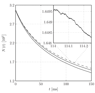
Figure 1: Total particle numbers for the sample trajectories of the system described in the text. Main plot shows the populations for (higher and lower solid lines) $v_{\rm cut}=\left\{44.3,59.1\right\}$ mms^-1, together with the results for the simple model (dashed line). The inset shows the population for the trajectory with $v_{\rm cut}=44.3$ mms^-1 over a subset of the total time.

IV Conclusion

The truncated Wigner description of ultracold Bose gases has many significant advantages over more traditional approaches, such as the Gross-Pitaevskii equation, and the extension outlined in this paper allows for the inclusion of three-body recombination processes. We have shown that within the validity regime of the Wigner truncation for two-body scattering, three-body recombination can be described using stochastic differential equations describing the evolution of a single trajectory, which can be solved using numerical techniques.

Appendix A Mathematical details

Using the particular Wigner function given by Eq. (16) in the full three-body recombination Wigner function equation of motion, Eq. (15), and evaluating all $\partial/\partial\alpha_{j},\partial/\partial\alpha_{j}^{*}$ operators returns

$$\frac{\partial W}{\partial t}^{\left({\rm TBR}\right)} = \gamma\int d{\bf x}\left\{-\left[\left(\xi_{\mathcal{P}}^{*}-\xi_{\mathcal{P}_{0}}^{*}\right)\Psi_{\mathcal{P}}+\Psi_{\mathcal{P}}^{*}\left(\xi_{\mathcal{P}}-\xi_{\mathcal{P}_{0}}\right)\right]\left(\left|\Psi_{\mathcal{P}}\right|^{4}-3\left|\Psi_{\mathcal{P}}\right|^{2}\delta_{\mathcal{P}}+\frac{3}{2}\delta_{\mathcal{P}}^{2}\right)\right.$$ (44a)

$$\mbox{}+\left(3\left|\Psi_{\mathcal{P}}\right|^{4}-6\left|\Psi_{\mathcal{P}}\right|^{2}\delta_{\mathcal{P}}+\frac{3}{2}\delta_{\mathcal{P}}^{2}\right)\delta_{\mathcal{P}}$$

$$({\rm 2nd}) \mbox{}-\left[\left(\xi_{\mathcal{P}}^{*}-\xi_{\mathcal{P}_{0}}^{*}\right)\Psi_{\mathcal{P}}-\Psi_{\mathcal{P}}^{*}\left(\xi_{\mathcal{P}}-\xi_{\mathcal{P}_{0}}\right)\right]\left(6\left|\Psi_{\mathcal{P}}\right|^{2}-6\delta_{\mathcal{P}}\right)\delta_{\mathcal{P}}+\left(6\left|\Psi_{\mathcal{P}}\right|^{2}-3\delta_{\mathcal{P}}\right)\delta_{\mathcal{P}}^{2}$$ (44b)

$$\mbox{}+\left(6\left|\Psi_{\mathcal{P}}\right|^{4}-12\left|\Psi_{\mathcal{P}}\right|^{2}\delta_{\mathcal{P}}+3\delta_{\mathcal{P}}^{2}\right)\left(\left|\xi_{\mathcal{P}}-\xi_{\mathcal{P}_{0}}\right|^{2}-\frac{1}{2}\sum_{j\in L}\frac{\Gamma_{j}}{2}\left|\psi_{j}\right|^{2}\right)$$

$$({\rm 3rd}) \mbox{}+\frac{3}{2}\left[\left(\xi_{\mathcal{P}}^{*}-\xi_{\mathcal{P}_{0}}^{*}\right)^{2}\Psi_{\mathcal{P}}^{2}+\Psi_{\mathcal{P}}^{*2}\left(\xi_{\mathcal{P}}-\xi_{\mathcal{P}_{0}}\right)^{2}\right]\delta_{\mathcal{P}}$$ (44c)

$$\mbox{}-3\left[\left(\xi_{\mathcal{P}}^{*}-\xi_{\mathcal{P}_{0}}^{*}\right)\Psi_{\mathcal{P}}+\Psi_{\mathcal{P}}^{*}\left(\xi_{\mathcal{P}}-\xi_{\mathcal{P}_{0}}\right)\right]\left[\left|\Psi_{\mathcal{P}}\right|^{2}\left(\left|\xi_{\mathcal{P}}-\xi_{\mathcal{P}_{0}}\right|^{2}-\sum_{j\in L}\frac{\Gamma_{j}}{2}\left|\psi_{j}\right|^{2}\right)\right.$$

$$\mbox{}\left.\hskip 28.45274pt+\delta_{\mathcal{P}}\left(\left|\xi_{\mathcal{P}}-\xi_{\mathcal{P}_{0}}\right|^{2}-\frac{1}{2}\sum_{j\in L}\frac{\Gamma_{j}}{2}\left|\psi_{j}\right|^{2}-\frac{3}{2}\delta_{P}\right)\right]$$

$$\mbox{}+6\left|\Psi_{\mathcal{P}}\right|^{2}\delta_{\mathcal{P}}\left(2\left|\xi_{\mathcal{P}}-\xi_{\mathcal{P}_{0}}\right|^{2}-\sum_{j\in L}\frac{\Gamma_{j}}{2}\left|\psi_{j}\right|^{2}\right)-3\delta_{\mathcal{P}}^{2}\left(2\left|\xi_{\mathcal{P}}-\xi_{\mathcal{P}_{0}}\right|^{2}+\frac{1}{2}\sum_{j\in L}\frac{\Gamma_{j}}{2}\left|\psi_{j}\right|^{2}-\frac{1}{2}\delta_{\mathcal{P}}\right)$$

$$({\rm 4th}) \mbox{}+\left[\left(\xi_{\mathcal{P}}^{*}-\xi_{\mathcal{P}_{0}}^{*}\right)^{2}\Psi_{\mathcal{P}}^{2}+\Psi_{\mathcal{P}}^{*2}\left(\xi_{\mathcal{P}}-\xi_{\mathcal{P}_{0}}\right)^{2}\right]\left(2\left|\xi_{\mathcal{P}}-\xi_{\mathcal{P}_{0}}\right|^{2}-3\sum_{j\in L}\frac{\Gamma_{j}}{2}\left|\psi_{j}\right|^{2}\right)$$ (44d)

$$\mbox{}-\left[\left(\xi_{\mathcal{P}}^{*}-\xi_{\mathcal{P}_{0}}^{*}\right)\Psi_{\mathcal{P}}+\Psi_{\mathcal{P}}^{*}\left(\xi_{\mathcal{P}}-\xi_{\mathcal{P}_{0}}\right)\right]\left(6\left|\xi_{\mathcal{P}}-\xi_{\mathcal{P}_{0}}\right|^{2}-6\sum_{j\in L}\frac{\Gamma_{j}}{2}\left|\psi_{j}\right|^{2}\right)\delta_{\mathcal{P}}$$

$$\mbox{}+\left(6\left|\xi_{\mathcal{P}}-\xi_{\mathcal{P}_{0}}\right|^{2}-3\sum_{j\in L}\frac{\Gamma_{j}}{2}\left|\psi_{j}\right|^{2}\right)\delta_{\mathcal{P}}^{2}$$

$$({\rm 5th}) \mbox{}-\left[\left(\xi_{\mathcal{P}}^{*}-\xi_{\mathcal{P}_{0}}^{*}\right)\Psi_{\mathcal{P}}+\Psi_{\mathcal{P}}^{*}\left(\xi_{\mathcal{P}}-\xi_{\mathcal{P}_{0}}\right)\right]\left(\left|\xi_{\mathcal{P}}-\xi_{\mathcal{P}_{0}}\right|^{2}-\sum_{j\in L}\frac{\Gamma_{j}}{2}\left|\psi_{j}\right|^{2}\right)^{2}$$ (44e)

$$\mbox{}+\left[3\left|\xi_{\mathcal{P}}-\xi_{\mathcal{P}_{0}}\right|^{4}-6\left|\xi_{\mathcal{P}}-\xi_{\mathcal{P}_{0}}\right|^{2}\sum_{j\in L}\frac{\Gamma_{j}}{2}\left|\psi_{j}\right|^{2}+\frac{3}{2}\left(\sum_{j\in L}\frac{\Gamma_{j}}{2}\left|\psi_{j}\right|^{2}\right)^{2}\right]\delta_{\mathcal{P}}$$

$$({\rm 6th}) \mbox{}+\frac{3}{2}\left|\xi_{\mathcal{P}}-\xi_{\mathcal{P}_{0}}\right|^{6}-3\left|\xi_{\mathcal{P}}-\xi_{\mathcal{P}_{0}}\right|^{4}\sum_{j\in L}\frac{\Gamma_{j}}{2}\left|\psi_{j}\right|^{2}$$ (44f)

$$\mbox{}\left.+3\left|\xi_{\mathcal{P}}-\xi_{\mathcal{P}_{0}}\right|^{2}\left(\sum_{j\in L}\frac{\Gamma_{j}}{2}\left|\psi_{j}\right|^{2}\right)^{2}-\left(\sum_{j\in L}\frac{\Gamma_{j}}{2}\left|\psi_{j}\right|^{2}\right)^{3}\right\}W.$$

Here the terms arising from the separate derivative orders are kept separated, as indicated on the left-hand side (first order derivative terms are given on the first and second lines). For compactness we have written $\delta_{\mathcal{P}}=\delta_{\mathcal{P}}\left({\bf x,x}\right)$.

References

- (1) A. J. Moerdijk, H. M. J. M. Boesten, and B. J. Verhaar, Phys. Rev. A 53, 916 (1996).
- (2) E. A. Burt et al., Phys. Rev. Lett. 79, 337 (1997).
- (3) J. Söding et al., App. Phys. B 69, 257 (1999).
- (4) B. D. Esry, C. H. Greene, and J. P. Burke, Jr., Phys. Rev. Lett. 83, 1751 (1999).
- (5) K. B. Davis et al., Phys. Rev. Lett. 75, 3969 (1995).
- (6) A. A. Norrie, R. J. Ballagh, and C. W. Gardiner, Submitted.
- (7) M. W. Jack, Phys. Rev. Lett. 89, 140402 (2002).
- (8) D. F. Walls and G. J. Milburn, Quantum Optics (Springer-Verlag, Berlin, 1994).
- (9) C. W. Gardiner and P. Zoller, Quantum Noise, 3rd ed. (Springer-Verlag, Berlin, 2004).
- (10) M. J. Steel et al., Phys. Rev. A 58, 4824 (1998).
- (11) C. W. Gardiner, Handbook of Stochastic Methods, 3rd ed. (Springer-Verlag, Berlin, 2004).
- (12) L. Pitaevskii and S. Stringari, Bose-Einstein Condensation (Oxford University Press, Oxford, 2003).
- (13) P. O. Fedichev, M. W. Reynolds, and G. V. Shlyapnikov, Phys. Rev. Lett. 77, 2921 (1996).
- (14) D. M. Stamper-Kurn et al., Phys. Rev. Lett. 80, 2027 (1998).
- (15) J. Stenger et al., Phys. Rev. Lett. 82, 2422 (1999).
- (16) W. H. Press, S. A. Teukolsky, W. T. Vetterling, and B. P. Flannery, Numerical Recipes in C, 2nd ed. (Cambridge University Press, Cambridge, MA, 1992).
- (17) G. N. Milstein and M. V. Tretyakov, Stochastic Numerics for Mathematical Physics (Springer-Verlag, Berlin, 2004).