Quantum turbulence and correlations in Bose-Einstein condensate collisions

Abstract

We investigate numerically simulated collisions between experimentally realistic Bose-Einstein condensate wavepackets, within a regime where highly populated scattering haloes are formed. The theoretical basis for this work is the truncated Wigner method, for which we present a detailed derivation, paying particular attention to its validity regime for colliding condensates. This paper is an extension of our previous Letter Norrie2005a , and we investigate both single-trajectory solutions, which reveal the presence of quantum turbulence in the scattering halo, and ensembles of trajectories, which we use to calculate quantum-mechanical correlation functions of the field.

I Introduction

In the same way as a classical electromagnetic field obeying Maxwell’s equations arises as an assembly of photons all in the same quantum state, a Bose-Einstein condensate, composed of Bosonic atoms all in the same quantum state, behaves very much like a classical field $\Psi({\bf x},t)$, whose equation of motion is the Gross-Pitaevskii equation

$$i\hbar\frac{\partial\Psi\left(\mathbf{x},t\right)}{\partial t}=\left[-\frac{\hbar^{2}\nabla^{2}}{2m}+\frac{4\pi\hbar^{2}a}{m}\left|\Psi\left(\mathbf{x},t\right)\right|^{2}\right]\Psi\left(\mathbf{x},t\right).$$

The Gross-Pitaevskii equation has been extraordinarily successful in describing a wide range of the phenomena associated with Bose-Einstein condensates—nevertheless, there are phenomena in which the quantized nature of this field is important. For example, when two Bose-Einstein condensates collide at a sufficiently high velocity, a halo of elastically scattered atoms is produced Chikkatur2000a ; Katz2002a ; Vogels2002a . The Gross-Pitaevskii equation with initial conditions corresponding to two Bose-Einstein condensates does not predict this scattering—it is a direct effect of the fact that the quantized field consists of interacting particles, and at its most elementary level, this halo is simply the result of elastic scattering of the constituent particles in the Bose-Einstein condensate.

A description of this phenomenon by means of the phenomenological inclusion of loss terms Band2000a , in a way reminiscent of the Boltzmann equation, was successful for collisions of smaller condensates, but seriously under-estimated the scattering for higher condensate densities. This underestimation arises because at high condensate densities, the final states into which the scattering occurs can become sufficiently highly occupied to cause Bosonic stimulation, which a simple Boltzmann treatment cannot produce. On the other hand, a treatment in terms of linearized quantum field theory Bach2002a ; Yurovsky2002a can deal with the Bosonic stimulation effects of highly occupied final states, but, being linearized, can treat neither the effects of large depletion, nor the essentially classical nonlinearity effects so well handled by the Gross-Pitaevskii equation.

An alternative method is the truncated Wigner method. This is a treatment of quantum field theory in which quantum mechanics is simulated by a classical random process. The method is approximate, but nevertheless very useful, both for quantum optical systems, where the field under consideration is the electromagnetic field, and for Bose-Einstein condensates, where the matter-wave field is under consideration, and reproduces many quantum mechanical features, such as quantum correlation functions, of these systems. The application to Bose-Einstein condensates has been developed by several groups Steel1998a ; Stoof1999a ; Duine2001a ; Stoof2001a ; Davis2001b ; Davis2001a ; Sinatra2001a ; Goral2001a ; Gardiner2002a ; Davis2002a ; Goral2002a ; Schmidt2003a with considerable success.

In qualitative terms, the truncated Wigner method provides a description of quantum field theory based on the Gross-Pitaevskii equationin which quantum mechanical vacuum fluctuations are simulated by by adding appropriate classical fluctuations in addition to the coherent field of the initial state of the Bose-Einstein condensate. These amount to half a quantum per degree of freedom, corresponding to the zero point energy of the harmonic oscillator which represents each mode of the field—the precise way in which this is done is presented in Sect.II.3.2. The elastic scattering effects which are not produced directly by a solution of the Gross-Pitaevskii equation for a coherent initial condensate field now appear as four-wave mixing between the coherent condensate field and the simulated vacuum fluctuations.

Since the number of modes in a local quantum field theory is infinite, the addition of a half a quantum per mode does in principle introduce a infinite density of vacuum fluctuations. Nevertheless, this does not invalidate the method. In practice what is used for the description of a Bose-Einstein condensate is an effective field theoryBraaten1999a ; Andersen2004a , valid only on a rather coarse spatial scale. Because of this, one can use a quantum field theory which contains only modes up to a certain cutoff value of the momentum, with an appropriately renormalized interaction. In a practical implementation of a cutoff field theory, one uses the standard contact interaction, with strength proportional to the scattering length, with corrections which depend on the size of the momentum cutoff. The density of added vacuum fluctuations is then quite finite, but cutoff dependent. The cutoff dependent effects of the vacuum fluctuations are then compensated by the cutoff dependent interaction strength. In simulations we must introduce this cutoff explicitly—in practice, for the choices of parameters we make, the cutoff corrections are 0.5% —see Sects.II.1.2, IV.1.

A related approach, the positive-P method Steel1998a ; Drummond1999a , (and its generalization, the gauge positive-P method) has also proven useful in describing Bose-condensed systems. Both the truncated Wigner and positive-P methods are examples of the general class of “classical field methods” well known in quantum optics Gardiner2000a . The positive-P methods are in principle exact, but are still difficult to implement for the kind of system we are considering here. However, technical progress is currently being made Deuar2006a ; Deuar2005a , and there does seem to be real promise that these exact methods will become practical.

We recently applied the truncated Wigner method to the problem of colliding condensates Norrie2005a , showing that it was feasible to simulate a realistic three-dimensional system and produce quantitative results. The aim of this paper is to expand upon and extend the treatment presented in there. To this end we provide here:

• A detailed derivation of the truncated Wigner method for colliding condensates, including a heuristic demonstration of how we can justify the neglect of terms arising in a Wigner function treatment of the problem, setting up the foundation of the method. We show in Sects.II.2.2–II.2.3 that for this kind of problem, the validity criterion for the method is that the density of the condensate (in co-ordinate space) must be very large compared with the density of the added quantum fluctuations.

• A treatment of the computational aspects of the problem, which are rather subtle. The main feature to note is that the cutoff necessary in the effective field theory cannot be simply provided by the fineness of the spatial grid used for computations. Rather, in order to avoid aliasing, it must be provided explicitly by means of a projector.

• The evaluation of averages using full ensemble computations. In Norrie2005a we evaluated averages using single computational runs, and averaging over regions of space where symmetry indicated the physics was the same. The results of our ensemble methods can provide additional information on coherence properties of the final states.

• Results which can be compared with feasible experiments. At present there are no experimental data which can be quantitatively compared with the results of this paper. The work was motivated by the observation of a strong halo in Vogels2002a , but no detailed measurements were made on this halo which could be compared with theory—furthermore, the parameter regime is not fully within the range of validity of our methodology. The work reported in Katz2005a has adapted our theoretical methodology to analyze a related experiment, and got good agreement. However, the calculation done was only two-dimensional, and therefore can only be regarded as indicative.

  For this paper we have chosen a parameter regime which is experimentally attainable, which is in the region where strong Bosonic stimulation is important, and which is fully within the region of validity of our methodology. In Sect.IV we give the values of appropriate parameters for both sodium and rubidium condensates. The numerical results are presented in SI units for a sodium condensate, and should be directly verifiable experimentally.

II Truncated Wigner method

In dilute Bose gases the appropriate Schrödinger picture Hamiltonian is

$$\hat{H} = \int d{\bf x}\,\hat{\Psi}^{\dagger}\left({\bf x}\right)\left\{-\frac{\hbar^{2}\nabla^{2}}{2m}+U_{\rm ext}\left({\bf x}\right)\right.$$ (1)

$$\left.\mbox{}+\frac{1}{2}\int d{\bf x}^{\prime}\,\hat{\Psi}^{\dagger}\left({\bf x}^{\prime}\right)U_{\rm 2b}\left({\bf x}-{\bf x}^{\prime}\right)\hat{\Psi}\left({\bf x}^{\prime}\right)\right\}\hat{\Psi}\left({\bf x}\right).$$

Here the external potential is $U_{\rm ext}\left({\bf x}\right)$ and pairwise interactions between the bosons are characterized by the two-body scattering potential $U_{\rm 2b}\left({\bf x-x}^{\prime}\right)$. The second-quantized field operator $\hat{\Psi}\left({\bf x}\right)$ annihilates a particle from position ${\bf x}$ and obeys the equal time commutation relations for identical bosons

$$\left[\hat{\Psi}\left({\bf x}\right),\hat{\Psi}\left({\bf x}^{\prime}\right)\right] = \left[\hat{\Psi}^{\dagger}\left({\bf x}\right),\hat{\Psi}^{\dagger}\left({\bf x}^{\prime}\right)\right]=0$$

$$\left[\hat{\Psi}\left({\bf x}\right),\hat{\Psi}^{\dagger}\left({\bf x}^{\prime}\right)\right] = \delta\left({\bf x}-{\bf x}^{\prime}\right),$$ (2)

where $\delta\left({\bf x}\right)$ is the three-dimensional Dirac delta function.

II.1 Effective field theory

II.1.1 Restricted basis field

We now decompose the field operator onto a single-particle basis

$$\hat{\Psi}\left({\bf x}\right)=\sum_{j}\psi_{j}\left({\bf x}\right)\hat{a}_{j},$$ (3)

where the mode operators obey the usual bosonic commutation relations

$$\left[\hat{a}_{i},\hat{a}_{j}\right]=\left[\hat{a}_{i}^{\dagger},\hat{a}_{j}^{\dagger}\right]=0,\hskip 14.22636pt\left[\hat{a}_{i},\hat{a}_{j}^{\dagger}\right]=\delta_{i,j}.$$ (4)

By choosing the basis set to be the orthonormal eigenstates of the non-interacting portion of the Hamiltonian, Eq. (1), i.e.

$$\left\{-\frac{\hbar^{2}\nabla^{2}}{2m}+U_{\rm ext}\left({\bf x}\right)\right\}\psi_{j}\left({\bf x}\right)=\hbar\omega_{j}\psi_{j}\left({\bf x}\right),$$ (5)

the full Hamiltonian, Eq. (1) can be rewritten as

$$\hat{H}=\sum_{j}\hbar\omega_{j}\hat{a}^{\dagger}_{j}\hat{a}_{j}+\frac{1}{2}\sum_{jrst}\left\langle jr\left|U_{\rm 2b}\right|st\right\rangle\hat{a}_{j}^{\dagger}\hat{a}_{r}^{\dagger}\hat{a}_{s}\hat{a}_{t}.$$ (6)

It is usual to simplify the Hamiltonian, Eq. (6), by using an effective field theory, obtained by eliminating higher energy modes, whose time-dependence is so rapid as to be unobservable in experiments on ultra cold gases. This kind of procedure has a long history, and takes many different forms. The description most appropriate to our methodology was given by Morgan Morgan2000a , and divides the modes $j$ into two sets, low- ($L$) and high-energy ($H$) subspaces depending on whether $\hbar\omega_{j}$ is less than or greater than a certain boundary energy $\varepsilon_{\rm cut}$. Provided $\varepsilon_{\rm cut}$ is sufficiently small, the effective Hamiltonian describing the $M$ low-energy modes can be found from Eq. (6) to be

$$\hat{H}_{\rm eff}=\sum_{j\in L}\hbar\omega_{j}\hat{a}^{\dagger}_{j}\hat{a}_{j}+\frac{U_{0}}{2}\sum_{jrst\in L}\left\langle jr|st\right\rangle\hat{a}_{j}^{\dagger}\hat{a}_{r}^{\dagger}\hat{a}_{s}\hat{a}_{t},$$ (7)

where the interaction parameter is defined as $U_{0}\equiv 4\pi\hbar^{2}a/m$ for the $s$-wave scattering length $a$.

II.1.2 Validity of the effective field theory

In order for $\hat{H}_{\rm eff}$ to accurately describe the low-energy subspace, $\varepsilon_{\rm cut}$ must be chosen so that the evolution of the high-energy modes is rapid compared to the evolution of the low-energy system, and $L$ must include enough modes to adequately describe the system dynamics. For the colliding systems we treat here, the low-energy subspace must be sufficiently large to contain all the modes required to represent the two colliding condensates and the scattering halo, as well as all the modes that can be directly involved in scattering events with those (condensate and halo) modes. In principle, this may conflict with the requirement that $\varepsilon_{\rm cut}$ be small — however in the cases we consider here, the error is less than a few percent, as we describe in section IV.

II.1.3 Projector representation

It is useful to have some formal manner of decomposing arbitrary objects, such as field operators or wavefunctions, into components on either side of the boundary energy. To this end we define the orthogonal projection operators (projectors)

$$\mathcal{P}\equiv\sum_{j\in L}\left|j\right\rangle\left\langle j\right|,\hskip 14.22636pt\mathcal{Q}\equiv\sum_{j\in H}\left|j\right\rangle\left\langle j\right|,$$ (8)

where $\mathcal{P}$ and $\mathcal{Q}$ act, respectively, as projectors onto the low- ($L$) and high-energy ($H$) subspaces. As these two subspaces completely span the infinite mode space, the projectors $\mathcal{P}$ and $\mathcal{Q}$ satisfy the closure relation $\mathcal{P}+\mathcal{Q}=1$.

In its coordinate space form, the low-energy projector acts on the arbitrary function $f\left({\bf x}\right)$ as

$$\mathcal{P}\left[f\left({\bf x}\right)\right]=\sum_{j\in L}\psi_{j}\left({\bf x}\right)\int d{\bf x}^{\prime}\psi_{j}^{*}\left({\bf x}^{\prime}\right)f\left({\bf x}^{\prime}\right).$$ (9)

Applying this to the field operator given by Eq. (3) returns the restricted field operator

$$\mathcal{P}\left[\hat{\Psi}\left({\bf x}\right)\right]=\sum_{j\in L}\psi_{j}\left({\bf x}\right)\hat{a}_{j}\equiv\hat{\Psi}_{\mathcal{P}}\left({\bf x}\right),$$ (10)

which is the component of the total field operator acting within the low-energy subspace. Because of the restricted nature of $\hat{\Psi}_{\mathcal{P}}$, the commutation relations given by Eq. (II) no longer apply. Rather it can be shown, using the mode operator commutation relations (4), that the restricted field operator obeys the equal time relations

$$\left[\hat{\Psi}_{\mathcal{P}}\left({\bf x}\right),\hat{\Psi}_{\mathcal{P}}\left({\bf x}^{\prime}\right)\right] = \left[\hat{\Psi}_{\mathcal{P}}^{\dagger}\left({\bf x}\right),\hat{\Psi}_{\mathcal{P}}^{\dagger}\left({\bf x}^{\prime}\right)\right]=0$$

$$\left[\hat{\Psi}_{\mathcal{P}}\left({\bf x}\right),\hat{\Psi}_{\mathcal{P}}^{\dagger}\left({\bf x}^{\prime}\right)\right] = \delta_{\mathcal{P}}\left({\bf x},{\bf x}^{\prime}\right),\hskip 28.45274pt$$ (11)

where we have defined the restricted delta function

$$\delta_{\mathcal{P}}\left({\bf x},{\bf x}^{\prime}\right)\equiv\sum_{j\in L}\psi_{j}^{*}\left({\bf x}^{\prime}\right)\psi_{j}\left({\bf x}\right).$$ (12)

Unlike the true (Dirac) delta function, the restricted delta function is spatially nonlocal, where the range of this nonlocality scales as $\varepsilon_{\rm cut}^{-1/2}$.

II.2 Wigner function evolution

Let us define the density operator of the restricted basis field to be $\rho\left(t\right)$, whose time evolution, using Eq. (7), is given by

$$i\hbar\frac{d\rho}{dt} = \left[\hat{H}_{\rm eff},\rho\right]$$ (14)

$$= \sum_{j\in L}\hbar\omega_{j}\left(\hat{a}_{j}^{\dagger}\hat{a}_{j}\rho-\rho\hat{a}_{j}^{\dagger}\hat{a}_{j}\right)$$

$$\mbox{}+\frac{U_{0}}{2}\sum_{jrst\in L}\left\langle jr|st\right\rangle\left(\hat{a}_{j}^{\dagger}\hat{a}_{r}^{\dagger}\hat{a}_{s}\hat{a}_{t}\rho-\rho\hat{a}_{j}^{\dagger}\hat{a}_{r}^{\dagger}\hat{a}_{s}\hat{a}_{t}\right),$$

The formulation of the truncated Wigner method is made using a multimode Wigner function representation of the density operator $\rho\left(t\right)$. The full details of how this is used are given in Gardiner2000a , and in brief are as follows. For a single mode, the Wigner function $W\left(\alpha,\alpha^{*},t\right)$ is defined in terms of the Wigner characteristic function

$$\chi_{W}\left(\lambda,\lambda^{*}\right)\equiv{\rm Tr}\left\{\rho\exp\left(\lambda\hat{a}^{\dagger}-\lambda^{*}\hat{a}\right)\right\},$$ (15)

as a Fourier transform

$$W(\alpha,\alpha^{*})=\frac{1}{\pi^{2}}\int d^{2}\lambda\,\exp\left(-\lambda\alpha^{*}+\lambda^{*}\alpha\right)\chi_{W}(\lambda,\lambda^{*}).$$ (16)

The Wigner function exists for any density operator, and its moments are equal to those of the symmetrized operator products:

$$\left\langle\left\{\hat{a}^{r}\left(\hat{a}^{\dagger}\right)^{s}\right\}_{\rm sym}\right\rangle = \int d^{2}\alpha\,\alpha^{r}\left(\alpha^{*}\right)^{s}W\left(\alpha,\alpha^{*}\right)$$ (17)

$$\equiv \left\langle\alpha^{r}\left(\alpha^{*}\right)^{s}\right\rangle_{W}.$$ (18)

The Wigner function is not guaranteed to be positive, but often is, and in these cases it behaves like a probability distribution for the variables $\alpha$, $\alpha^{*}$.

The action of the mode operators $\hat{a},\hat{a}^{\dagger}$ on the density operator can be expressed as the action of differential operators on the Wigner function using the operator correspondences, which follow from Eq. (16)

$$\hat{a}\rho\left(t\right) \leftrightarrow \left(\alpha+\frac{1}{2}\frac{\partial}{\partial\alpha^{*}}\right)W\left(\alpha,\alpha^{*},t\right)$$ (19a)

$$\hat{a}^{\dagger}\rho\left(t\right) \leftrightarrow \left(\alpha^{*}-\frac{1}{2}\frac{\partial}{\partial\alpha}\right)W\left(\alpha,\alpha^{*},t\right)$$ (19b)

$$\rho\left(t\right)\hat{a} \leftrightarrow \left(\alpha-\frac{1}{2}\frac{\partial}{\partial\alpha^{*}}\right)W\left(\alpha,\alpha^{*},t\right)$$ (19c)

$$\rho\left(t\right)\hat{a}^{\dagger} \leftrightarrow \left(\alpha^{*}+\frac{1}{2}\frac{\partial}{\partial\alpha}\right)W\left(\alpha,\alpha^{*},t\right).$$ (19d)

The extension to many modes is straightforward.

For the restricted basis von Neumann equation, Eq. (14), we find using these operator correspondences that the evolution of the multimode Wigner function $W\left(\left\{\alpha_{j},\alpha_{j}^{*}\right\},t\right)$ is given by

$$i\hbar\frac{\partial W}{\partial t} = -\sum_{j\in L}\hbar\omega_{j}\left(\frac{\partial}{\partial\alpha_{j}}\alpha_{j}-\frac{\partial}{\partial\alpha_{j}^{*}}\alpha_{j}^{*}\right)W$$ (20)

$$\mbox{}-U_{0}\sum_{jrst\in L}\left\langle jr|st\right\rangle\left(\frac{\partial}{\partial\alpha_{j}}\alpha_{t}-\frac{\partial}{\partial\alpha_{t}^{*}}\alpha_{j}^{*}\right)\left(\alpha_{r}^{*}\alpha_{s}-\delta_{r,s}-\frac{1}{4}\frac{\partial^{2}}{\partial\alpha_{r}\partial\alpha_{s}^{*}}\right)W.$$

This Wigner function evolution is exactly equivalent to the von Neumann equation, Eq. (14).

II.2.1 Wigner truncation

Equations of motion for the Wigner function of the form given by Eq. (20) are well known, particularly in quantum optics Gardiner2000a , and even in the case of a few variables are not easy to solve numerically. The Wigner truncation, in which the third-order derivative terms are dropped, has often been made, since the resulting equation of motion, having only first-order derivatives on the right, is of the form of a Liouville equation. It thus describes an ensemble of trajectories obeying an equation of motion which is essentially classical, and which can be simulated relatively straightforwardly.

The justification for this truncation is intuitively reasonable; if the quantum state of the system is such that it is “almost classical”, then the classical equation should prevail. One can present scaling arguments, in which it is assumed that the Wigner function behaves like a sharply peaked probability distribution centered around a macroscopic mean value of the parameters $\alpha_{j}$. These arguments can then be used to show that the contribution from the third-order derivative terms is negligible provided the mean values of all of the $\alpha_{j}$ are large. This kind of argument has been made relatively rigorously by Polkovnikov Polkovnikov2003a , who has shown how the third-order derivative terms give a correction to the classical trajectories.

In the case of colliding condensates this criterion is not valid. The initial state of the system is only highly occupied in the modes in the vicinity of the two incoming momenta, and we want to consider the evolution into a large number of initially unoccupied modes. However, experience in quantum optics shows that the Wigner truncation can be valid for such a system; the prime example is the degenerate parametric oscillator, in which two modes of the electromagnetic field are made to interact by means of a nonlinear crystal to give a Hamiltonian of the form

$$\hat{H}_{\rm dpo}=\hbar\omega\hat{a}^{\dagger}\hat{a}+2\hbar\omega\hat{b}^{\dagger}\hat{b}+g\left\{\hat{b}\left(\hat{a}^{\dagger}\right)^{2}+\hat{b}^{\dagger}\hat{a}^{2}\right\}.$$ (21)

Here $\hat{a}$ and $\hat{b}$ are destruction operators for field modes with frequencies $\omega$ and $2\omega$. A Wigner function treatment soon reveals an equation of motion with first- and third-order derivatives with respect to corresponding Wigner function variables $\alpha,\alpha^{*},\beta,\beta^{*}$.

In the relevant physical situation, the mode $\hat{a}$ is initially unpopulated and the mode $\hat{b}$ is derived from an intense laser, and as such is essentially a classical field — thus one makes the replacement

$$\hat{b}\rightarrow Be^{-2i\omega t},$$ (22)

where $B$ is a classical amplitude, and thus

$$\hat{H}_{\rm dpo}\rightarrow\hat{H}^{\prime}_{\rm dpo} = \hbar\omega\hat{a}^{\dagger}\hat{a}$$ (23)

$$\mbox{}+g\left\{Be^{-2i\omega t}\left(\hat{a}^{\dagger}\right)^{2}+B^{*}e^{2i\omega t}\hat{a}^{2}\right\}.$$

This approximate Hamiltonian produces a Wigner function equation of motion with only first-order derivatives with respect to $\alpha,\alpha^{*}$, and is well verified to give accurate physical predictions for the production of quanta in the mode $\hat{a}$.

Alternatively, one could simply drop the third-order terms in the Wigner function equation of motion, and one would get equivalent results in the limit that one could neglect depletion of the field $\hat{b}$. This is in spite of the fact that the occupation of the mode $\hat{a}$ is not large — thus it appears that it is sufficient for only some of the modes to be highly occupied for it to be valid to drop the third-order derivative terms.

II.2.2 Validity of the Wigner truncation for colliding condensates

The case of colliding condensates is analogous to that just discussed. There are a number of highly occupied modes—those corresponding to the original condensate packets, and a larger number of unoccupied modes. In the following we give a heuristic analysis of why the Wigner truncation should be acceptable for this system.

Consider a multimode Wigner function, which at some time $\tau$ is factorizable into single-mode functions, of the form

$$W\left(\left\{\alpha_{j},\alpha_{j}^{*}\right\},\tau\right)=\prod_{j\in L}\frac{\Gamma_{j}}{\pi}\exp\left[-\Gamma_{j}\left|\alpha_{j}-\alpha_{j_{0}}\right|^{2}\right],$$ (24)

where $\alpha_{j_{0}}$ gives the expectation value (coherent) amplitude of the $j$th mode, and $\Gamma_{j}\leq 2$ is the inverse width of the Wigner function. This Wigner function includes both thermal and coherent (for which $\Gamma_{j}=2$) statistics, but does not allow the modes to exist as pure number states or other more elaborate forms. In fact we use exactly this Wigner function when constructing the initial states of our simulations, for which we find that the modes display essentially Gaussian statistics at all times, with minimal correlations between the modes. Thus we expect the following analysis to be appropriate for the duration of the collisions considered here.

Substituting the Wigner function given by Eq. (24) into the nonlinear portion of Eq. (20) gives the evolution at time $\tau$ as

$$i\hbar\frac{\partial W}{\partial t}^{\rm(nonlin)} = U_{0}\sum_{jrst\in L}\left\langle jr|st\right\rangle\left[\Gamma_{j}\left(\alpha_{j}^{*}-\alpha_{j_{0}}^{*}\right)\alpha_{t}-\Gamma_{t}\alpha_{j}^{*}\left(\alpha_{t}-\alpha_{t_{0}}\right)\right]$$ (25)

$$\hskip 56.9055pt\times\left\{\left[\alpha_{r}^{*}\alpha_{s}-\delta_{r,s}\right]-\left[\frac{\Gamma_{r}\Gamma_{s}}{4}\left(\alpha_{r}^{*}-\alpha_{r_{0}}^{*}\right)\left(\alpha_{s}-\alpha_{s_{0}}\right)-\frac{\Gamma_{r}}{2}\delta_{r,s}\right]\right\}W.$$

Here the first bracketed set of terms within the braces arise from the first-order derivatives, while the second bracketed set of terms arise from the third-order derivatives.

Analogously to the definition of the restricted basis field operator, as given by Eq. (10), we define the classical wavefunction

$$\Psi_{\mathcal{P}}\left({\bf x}\right)\equiv\sum_{j\in L}\psi_{j}\left({\bf x}\right)\alpha_{j},$$ (26)

which represents a possible state of the total restricted basis field, including both the condensate and noncondensate particles, at any given time. We also define the related wavefunction

$$\xi_{\mathcal{P}}\left({\bf x}\right)\equiv\sum_{j\in L}\psi_{j}\left({\bf x}\right)\frac{\Gamma_{j}}{2}\alpha_{j},$$ (27)

whose expectation value, calculated using the Wigner function given by Eq. (24), is found to be

$$\xi_{\mathcal{P}_{0}}\left({\bf x}\right)\equiv\left\langle\xi_{\mathcal{P}}\left({\bf x}\right)\right\rangle_{W}=\sum_{j\in L}\psi_{j}\left({\bf x}\right)\frac{\Gamma_{j}}{2}\alpha_{j_{0}}.$$ (28)

Using these wavefunction forms in the Wigner function evolution, Eq. (25), gives

$$i\hbar\frac{\partial W}{\partial t}^{\rm(nonlin)} = 2U_{0}\int d{\bf x}\left[\left(\xi_{\mathcal{P}}^{*}-\xi_{\mathcal{P}_{0}}^{*}\right)\Psi_{\mathcal{P}}-\Psi_{\mathcal{P}}^{*}\left(\xi_{\mathcal{P}}-\xi_{\mathcal{P}_{0}}\right)\right]$$ (29)

$$\hskip 85.35826pt\times\left\{\left[\left|\Psi_{\mathcal{P}}\right|^{2}-\sum_{j\in L}\left|\psi_{j}\right|^{2}\right]-\left[\left|\xi_{\mathcal{P}}-\xi_{\mathcal{P}_{0}}\right|^{2}-\sum_{j\in L}\frac{\Gamma_{j}}{2}\left|\psi_{j}\right|^{2}\right]\right\}W.$$

where we have suppressed the explicit spatial dependences and have retained the ordering of Eq. (25).

To justify the Wigner truncation, we now show that the terms arising from the cubic derivatives in Eq. (29) are small compared with the first order derivative terms for all points ${\bf x}$ on the coordinate space field. This local analysis requires that the inequality

$$\left|\frac{\left|\xi_{\mathcal{P}}-\xi_{\mathcal{P}_{0}}\right|^{2}-\sum_{j\in L}\frac{\Gamma_{j}}{2}\left|\psi_{j}\right|^{2}}{\left|\Psi_{\mathcal{P}}\right|^{2}-\sum_{j\in L}\left|\psi_{j}\right|^{2}}\right|\ll 1,$$ (30)

should hold over all space. A useful quantitative description of the inequality is in terms of the distributional averages (classical expectation values), for which we find that

$$\left\langle\left|\xi_{\mathcal{P}}-\xi_{\mathcal{P}_{0}}\right|^{2}\right\rangle_{W}=\sum_{j\in L}\frac{\Gamma_{j}}{4}\left|\psi_{j}\right|^{2},$$ (31)

which is of similar magnitude to $\delta_{\mathcal{P}}\left({\bf x,x}\right)$, Eq. (12). For the expectation value of the $\left|\Psi_{\mathcal{P}}\right|^{2}$ however, a more useful representation can be obtained using the correspondence of Wigner function averages to the quantum expectation values, Eq. (17). We find that in the general case (i.e. irrespective of the particular form of the Wigner function)

$$\left\langle\left|\Psi_{\mathcal{P}}\left({\bf x}\right)\right|^{2}\right\rangle_{W}=n\left({\bf x}\right)+\frac{1}{2}\delta_{\mathcal{P}}\left({\bf x,x}\right),$$ (32)

where the total density of real particles $n\left({\bf x}\right)$ is defined using the restricted basis field operators by

$$n\left({\bf x}\right)\equiv\left\langle\hat{n}\left({\bf x}\right)\right\rangle=\left\langle\hat{\Psi}_{\mathcal{P}}^{\dagger}\left({\bf x}\right)\hat{\Psi}_{\mathcal{P}}\left({\bf x}\right)\right\rangle.$$ (33)

Using Eqs. (31,32), the validity criterion for the Wigner truncation, Eq. (30), becomes

$$\left|n\left({\bf x}\right)-\frac{1}{2}\delta_{\mathcal{P}}\left({\bf x,x}\right)\right|\gg\sum_{j\in L}\frac{\Gamma_{j}}{4}\left|\psi_{j}\left({\bf x}\right)\right|^{2}.$$ (34)

Thus in order to justify the truncation it is required that the real particle density is large compared with the commutator of the restricted field, $\delta_{\mathcal{P}}\left({\bf x,x}\right)$.

For a zero-temperature homogeneous field, such that $\Gamma_{j}=2$ for all modes, the validity condition becomes simply $N\gg M$, which is similar to that given by Sinatra et al. Sinatra2002a . However, for the inhomogeneous finite-temperature case, the localized truncation condition given by Eq. (34) is less easy to justify, especially when one considers that for these inhomogeneous fields there may be regions where the total particle density goes to zero. However, the part of the Wigner function evolution dependent upon interparticle scattering is significant in only those regions where there is a high particle density, i.e. the regions where the truncation is accurate, so that the truncation can be made over all space without adversely affecting the accuracy of the approximation. Interestingly, this justification relies on the relative magnitude of the particle and mode-function densities, rather than the numbers of particles and modefunctions. Thus it appears to be possible to accurately apply the Wigner truncation to systems in which there are significantly more basis modes than real particles.

II.2.3 Critique of the Validity Criterion

The validity criterion in the form Eq. (34), or in the form for a homogeneous system $N\gg M$, shows that for a given number of real particles in the system, accurate results will not result if the number of basis modes $M$ is too large. This is fundamental to the truncated Wigner function method, in which vacuum noise is added to every mode. Methods based on the P-functionDeuar2006a ; Deuar2005a ; Gardiner2000a do not have this problem, since noise is added dynamically and only to modes with real occupation. However, as noted in the introduction, other technical difficulties so far make these methods more difficult to use in practice.

II.2.4 Truncated Wigner function Fokker-Planck equation

Within the validity regime of the Wigner truncation the Wigner function evolution given by Eq. (20) is well approximated by the truncated Wigner function Fokker-Planck equation

$$i\hbar\frac{\partial W}{\partial t} \approx -\sum_{j\in L}\frac{\partial}{\partial\alpha_{j}}\left\{\hbar\omega_{j}\alpha_{j}+U_{0}\sum_{rst\in L}\left\langle jr|st\right\rangle\alpha_{r}^{*}\alpha_{s}\alpha_{t}\right\}W$$ (35)

$$\mbox{}+\sum_{j\in L}\frac{\partial}{\partial\alpha_{j}^{*}}\left\{\hbar\omega_{j}\alpha_{j}^{*}+U_{0}\sum_{rst\in L}\left\langle jr|st\right\rangle^{*}\alpha_{r}\alpha_{s}^{*}\alpha_{t}^{*}\right\}W.$$

Note that we have also removed from Eq. (35) the nonlinear evolution dependent upon $\delta_{r,s}$ (see Eq. (20)), which corresponds to terms dependent upon $\delta_{\mathcal{P}}\left({\bf x,x}\right)$ in coordinate space, and whose influence on the total evolution, as we discussed above, is negligible. Indeed, in order to preserve energy conservation these terms must be removed alongside the cubic derivative terms.

II.3 Ensemble differential equations

The Liouville equation, Eq. (35), gives the equation of motion for the ensemble of trajectories of the variables $\left\{\alpha_{j},\alpha_{j}^{*}\right\}$. The corresponding equations of motion for individual trajectories of the system are given by Gardiner2003b

$$i\hbar\frac{d\alpha_{j}}{dt}=\hbar\omega_{j}\alpha_{j}+U_{0}\sum_{rst\in L}\left\langle jr|st\right\rangle\alpha_{r}^{*}\alpha_{s}\alpha_{t},$$ (36)

where $j\in L$. Every distinct realization of the differential equation uses a different initial noise field, and hence yields a distinct trajectory in the phase space of the system — we describe appropriate initial states in section II.3.2.

By using our previously defined restricted basis wavefunction, Eq. (26), in the time-dependent form $\Psi_{\mathcal{P}}\left({\bf x},t\right)$, we can rewrite the evolution of the $j$th low-energy mode amplitude as

$$i\hbar\frac{d\alpha_{j}}{dt}=\hbar\omega_{j}\alpha_{j}+U_{0}\int d{\bf x}\,\psi_{j}^{*}\left|\Psi_{\mathcal{P}}\right|^{2}\Psi_{\mathcal{P}},$$ (37)

which we find to be convenient for numerical simulation. We use Eq. (37) (in a dimensionless form) to calculate the central results of this paper.

Note that although our differential equations are not stochastic differential equations, they do have a stochastic nature that arises from the random component of the initial field.

II.3.1 Projected form of the differential equations

It is instructive to obtain the differential equation for the entire restricted field, rather than the evolutions of the individual mode amplitudes. Again using the definition of the restricted basis wavefunction, we find that Eq. (37) gives rise to

$$i\hbar\frac{\partial\Psi_{\mathcal{P}}}{\partial t}=\left[-\frac{\hbar^{2}\nabla^{2}}{2m}+U_{\rm ext}\right]\Psi_{\mathcal{P}}+U_{0}\mathcal{P}\left\{\left[\left|\Psi_{\mathcal{P}}\right|^{2}\right]\Psi_{\mathcal{P}}\right\},$$ (38)

where we have replaced the basis eigenenergies with the corresponding diagonal Hamiltonian and have recognized the form of the projector onto the low-energy mode space, Eq. (9).

It is straightforwardly shown from any of Eqs. (36,37,38) that the normalization of the total field for a single trajectory, defined as

$$\mathcal{N}\equiv\sum_{j\in L}\left|\alpha_{j}\right|^{2}=\int d{\bf x}\left|\Psi_{\mathcal{P}}\right|^{2},$$ (39)

is strictly conserved, so that $d\mathcal{N}/dt=0$, as is the total field energy

$$\mathcal{E}=\sum_{j\in L}\hbar\omega_{j}\left|\alpha_{j}\right|^{2}+\frac{U_{0}}{2}\int d{\bf x}\,\left|\Psi_{\mathcal{P}}\right|^{4}.$$ (40)

Note that $\mathcal{N}$ and $\mathcal{E}$ are not the physically observable field population and energy, as they include contributions from the virtual particles (the noise). It could be imagined that the projector serves to remove those quanta that are shifted outside the low-energy subspace by pairwise collisions, reducing the total population of the field over time. This view is incorrect. Rather the projector simply disallows these processes, a result that is most easily seen from Eq. (36).

II.3.2 Initial states

As the ensemble differential equations contain no dynamic noise sources, to sample the evolution of the Wigner function we are obliged only to ensure that the ensemble of initial states yields the appropriate Wigner function. For the zero-temperature collisions presented here we assume an initial Wigner function of the form given by Eq. (24), where the modes are assumed to display uniformly coherent statistics, for which $\Gamma_{j}=2$ for all $j$. The corresponding initial state of the $j$th mode amplitude for a single trajectory is given by

$$\alpha_{j}\left(0\right)=\alpha_{j_{0}}\left(0\right)+\frac{1}{\sqrt{2\Gamma_{j}}}\left(A_{j}+iB_{j}\right).$$ (41)

Here, as before, $\alpha_{j_{0}}$ is the coherent amplitude of the mode, and can therefore be identified as the condensate amplitude for the $j$th mode. The quantities $A_{j},B_{j}$ are real independent Gaussian random variables of zero mean and unit variance, such that

$$\left\langle A_{j}\right\rangle=\left\langle B_{j}\right\rangle=\left\langle A_{i}B_{j}\right\rangle=0$$

$$\left\langle A_{i}A_{j}\right\rangle=\left\langle B_{i}B_{j}\right\rangle=\delta_{i,j}.$$ (42)

The equivalent coordinate space initial state is found using Eqs. (26,41) to be

$$\Psi_{\mathcal{P}}\left({\bf x},0\right) = \sum_{j\in L}\psi_{j}\left[\alpha_{j_{0}}\left(0\right)+\frac{1}{\sqrt{2\Gamma_{j}}}\left(A_{j}+iB_{j}\right)\right]$$ (43)

$$= \Psi_{\mathcal{P}_{0}}\left({\bf x},0\right)+\chi_{\mathcal{P}}\left({\bf x}\right).$$ (44)

Here $\Psi_{\mathcal{P}_{0}}=\left\langle\Psi_{\mathcal{P}}\right\rangle_{W}$ is the coherent field amplitude, i.e. the condensate wavefunction. The spatial fluctuations, $\chi_{\mathcal{P}}$ are found from Eq. (II.3.2) to satisfy

$$\left\langle\chi_{\mathcal{P}}\right\rangle = 0,$$ (45)

$$\left\langle\chi_{\mathcal{P}}^{*}\left({\bf x}^{\prime}\right)\chi_{\mathcal{P}}\left({\bf x}\right)\right\rangle = \sum_{j\in L}\frac{1}{\Gamma_{j}}\psi_{j}^{*}\left({\bf x}^{\prime}\right)\psi_{j}\left({\bf x}\right),$$ (46)

where Eq. (46) can be seen to be similar to the restricted delta function defined by Eq. (12), and proportional to it when all $\Gamma_{j}=2$. For our uniformly coherent initial state we find that the expected total field normalization, as given by Eq. (39), is

$$\left\langle\mathcal{N}\right\rangle=N_{0}\left(0\right)+\frac{M}{2},$$ (47)

where

$$N_{0}\left(t\right)\equiv\sum_{j\in L}\left|\alpha_{j_{0}}\left(t\right)\right|^{2}=\int d{\bf x}\left|\Psi_{\mathcal{P}_{0}}\left({\bf x},t\right)\right|^{2},$$ (48)

is the total number of condensate particles and, as before, $M$ is the number of low-energy modes. Although the number of condensate particles is in general not conserved, the total number of real particles $N$ is conserved.

III Numerical methods

III.1 Computational units

It is convenient for the purposes of numerical simulation to express the equations in dimensionless computational units. The systems we treat are initially confined within a harmonic potential

$$U_{\rm harm}\left({\bf x}\right)=\frac{m}{2}\left(\omega_{x}^{2}x^{2}+\omega_{y}^{2}y^{2}+\omega_{z}^{2}z^{2}\right),$$ (49)

which provides

$$x_{0}=\sqrt{\frac{\hbar}{2m\omega_{x}}},\hskip 14.22636ptt_{0}=\frac{1}{\omega_{x}},\hskip 14.22636pt\varepsilon_{0}=\hbar\omega_{x}.$$ (50)

as a natural choice of units for length, time and energy respectively.

In these units Eq. (37), becomes

$$i\frac{d\alpha_{j}}{d\tilde{t}}=\tilde{\omega}_{j}\alpha_{j}+\tilde{U}_{0}\int d\tilde{\bf x}\,\tilde{\psi}_{j}^{*}\left|\tilde{\Psi}_{\mathcal{P}}\right|^{2}\tilde{\Psi}_{\mathcal{P}},$$ (51)

where we have used tildes to indicate quantities in computational units ($\alpha_{j}$ is identical in both computational and S.I. units). As an example, the dimensionless interaction parameter $\tilde{U}_{0}$ is

$$\tilde{U}_{0}\equiv\frac{U_{0}}{\varepsilon_{0}x_{0}^{3}}=8\pi a\sqrt{\frac{2m\omega_{x}}{\hbar}}.$$ (52)

III.2 Plane wave basis

While our formalism allows the use of any set of orthonormal basis states $\psi_{j}\left({\bf x}\right)$, the most appropriate choice of basis for collisions occurring in free space is the plane wave states. We use a three-dimensional, periodically-bounded rectangular space of volume $V=L_{x}\times L_{y}\times L_{z}$, for which the (normalized to unity) plane-wave modes are

$$\psi_{j}\left({\bf x}\right)=\frac{1}{\sqrt{V}}e^{i{\bf k}_{j}\cdot{\bf x}}.$$ (53)

Here the wavevector ${\bf k}_{j}$ associated with the $j$th mode is

$${\bf k}_{j}=\frac{2\pi m_{j}}{L_{x}}\hat{\bf k}_{x}+\frac{2\pi n_{j}}{L_{y}}\hat{\bf k}_{y}+\frac{2\pi p_{j}}{L_{z}}\hat{\bf k}_{z},$$ (54)

where $m_{j}$, $n_{j}$ and $p_{j}$ are integers.

In our dimensionless computational units, the single-particle energy of the $j$th mode is given by $\tilde{\omega_{j}}=\tilde{k}_{j}^{2}$, and the differential equation describing the evolution of the $j$th mode, Eq. (51), becomes

$$i\frac{d\alpha_{j}}{d\tilde{t}}=\tilde{k}_{j}^{2}\alpha_{j}+\frac{\tilde{U}_{0}}{\sqrt{\tilde{V}}}\int d\tilde{\bf x}\,e^{-i\tilde{\bf k}_{j}\cdot\tilde{\bf x}}\left|\tilde{\Psi}_{\mathcal{P}}\right|^{2}\tilde{\Psi}_{\mathcal{P}}.$$ (55)

We have previously defined the low-energy mode subspace $L$ to consist of all those modes whose energies are less than some cutoff energy $\varepsilon_{\rm cut}$. It is easily seen that for the plane-wave modes this energy cutoff is translated to a spherical cutoff in wavevector space. Thus the $L$ subspace consists of all those modes whose wavevectors satisfy $k_{j}\leq k_{\rm cut}$, where the cutoff wavenumber is defined (in computational units) as $\tilde{k}_{\rm cut}\equiv\sqrt{\tilde{\varepsilon}_{\rm cut}}$.

III.3 Propagation algorithm

To propagate the differential equations we employ a modified version of the Fourth-order Runge-Kutta in the Interaction Picture (RK4IP) algorithm Ballagh2000a , which has been used extensively to simulate the time-dependent Gross-Pitaevskii equation. The only difference in our equations of motion is the presence of the projector, which is straightforwardly performed in momentum space, albeit with a small number of required conditions that are worth stating explicitly.

Using a plane-wave basis, the conversions between coordinate space and mode space required by Eq. (55) are achieved using Fast Fourier Transform (FFT) algorithms Press1992a , which require that the two spaces are represented using identical numbers of rectangularly arranged grid points. Thus, given that the low-energy mode space is spherically bounded, we must include additional modes (from the $H$ subspace) to form a rectangularly bounded space (the padded mode-space). Using a padded mode space that tangentially bounds $L$ is not adequate, because with such a grid population scattered from the $L$ subspace into the $H$ subspace, which should be removed by the projector, can be aliased by the FFT back into the $L$ subspace, thereby adversely affecting the accuracy of the simulation. A rectangularly bounded mode-space grid of extent $4k_{\rm cut}\times 4k_{\rm cut}\times 4k_{\rm cut}$ is the smallest grid that prevents aliased components returning to the $L$ subspace, and therefore allows for accurate calculation of the low-energy subspace dynamics while minimizing computational memory requirements. This padded mode-space has $\sim 48/\pi$ times as many grid points as there are low-energy modes, and significant computational memory savings can be made by representing the $L$ subspace on the full padded grid only when absolutely necessary for the propagation algorithm.

IV System of interest

In our previous letter Norrie2005a we presented results obtained from a single trajectory describing a very similar collision to one that had been realized experimentally Ketterle2002a . However, careful analysis indicates that the systems presented in Norrie2005a may stretch the validity criteria of the truncated Wigner method, in particular due to an inappropriately low $k_{\rm cut}$. In this paper we treat colliding systems that probe a different region of parameter space, one which is both experimentally possible and well within the validity regime of our formalism.

The condensate part of our initial state (see Eq. (44)) is assumed to be composed of two equally populated wavepackets derived from a single harmonically trapped Bose-Einstein condensate using a short $\pi/2$ Bragg pulse Phillips1999a of wavevector $\left(\Delta q,0,0\right)$, so that

$$\Psi_{\mathcal{P}_{0}}\left({\bf x},t=0\right)=\frac{1}{\sqrt{2}}\Psi\left({\bf x}\right)\left[e^{+i\frac{\Delta q}{2}x}+e^{-i\frac{\Delta q}{2}x}\right],$$ (56)

where the envelope function $\Psi\left({\bf x}\right)$ is that of the initial, unscattered condensate wavefunction. We describe this envelope wavefunction by the $N_{0}$ atom ground state solution to the time-independent Gross-Pitaevskii equation. Eq. (56) assumes a centre-of-mass frame, which reduces the number of low-energy modes required and provides a convenient symmetry. We assume a zero-temperature initial state, such that the all modes are initially coherent and $N=N_{0}\left(t=0\right)$, and we remove the confining potential at $t=0$.

We use a (dimensionless) nonlinear parameter of $\tilde{U}_{0}=1\times 10^{-2}$, an initial (total) condensate population of two million, and a relative wavepacket wavenumber of $\tilde{\Delta q}=10$. This parameter set corresponds to a system of ²³Na atoms, initially confined within a potential with $\omega_{x}=2\pi\times 4.57$ Hz, where the wavepackets move with a relative speed of 4.0 mm s^-1, or alternatively to a ⁸⁷Rb system initially confined within a trap with $\omega_{x}=2\pi\times 0.31$ Hz, where the wavepackets are separating at 0.53 mm s^-1. We assume the trapping potential is cylindrically symmetric, with $\lambda\equiv\lambda_{z}/\lambda_{x,y}=\sqrt{8}$.

For our (dimensionless) parameter set, the Thomas-Fermi chemical potential Stringari1999a is found to be $\tilde{\mu}_{\rm TF}=21.4$, giving Thomas-Fermi radii of $\tilde{x}_{\rm TF}=\tilde{y}_{\rm TF}=2\sqrt{\tilde{\mu}_{\rm TF}}=9.24$ and $\tilde{z}_{\rm TF}=2\sqrt{\tilde{\mu}_{\rm TF}}/\lambda=3.27$. In order to enclose the colliding system until packet separation we find that a volume of $\tilde{V}=48.9\times 33.5\times 33.5$ is appropriate.

IV.1 Truncated Wigner method validity criteria

In restricting the system to the low-energy subspace, as described in section II.1.2, it was stated that the momentum space must be large enough to include all relevant modes to describe the evolution. For the colliding system this requirement translates to $k_{\rm cut}>3\Delta q/2$, such that all possible scattering events directly involving the initial condensate wavepackets and the halo are included. To meet this validity criterion we use a low-energy subspace cutoff of $\tilde{k}_{\rm cut}=18$, for which $M=5.4\times 10^{6}$. Using a result from Morgan1999a we find that the error in the $s$-wave scattering length in the effective Hamiltonian, Eq. (7), is approximately 0.5% for this value of the cutoff.

The second validity criterion for the truncated Wigner method, Eq. (34), is most easily expressed as

$$n\left({\bf x}\right)\gg\delta_{\mathcal{P}}\left({\bf x,x}\right).$$ (57)

For a harmonically trapped Thomas-Fermi condensate, the (dimensionless) maximum density is $\tilde{n}\left({\bf x}=0\right)=\tilde{\mu}_{\rm TF}/\tilde{U_{0}}$, so that for our system $\tilde{n}\left({\bf x}=0\right)=2140$. For a plane wave basis we find that the equiposition restricted delta function can be expressed as

$$\delta_{\mathcal{P}}\left({\bf x,x}\right)=\frac{M}{V}\approx\frac{k_{\rm cut}^{3}}{6\pi^{2}}.$$ (58)

For $\tilde{k}_{\rm cut}=18$, we find that $\tilde{\delta}_{\mathcal{P}}\left({\bf x,x}\right)\approx 100$, so that we expect the Wigner truncation criterion, Eq. (34), to be satisfied for this system.

We have simulated (otherwise identical) additional trajectories using a larger cutoff, $k_{\rm cut}=20.57$, for which $M=8.4\times 10^{6}$. Using the extrapolation method outlined in section V.2.3, we find that the difference in the calculated total coherent population between the system with this larger cutoff and our principal system approaches 1.25% by the end of the simulation times.

For the remainder of this paper we present all results in SI units, appropriate for the ²³Na system described above.

V Results

V.1 Single trajectory results

V.1.1 Momentum space

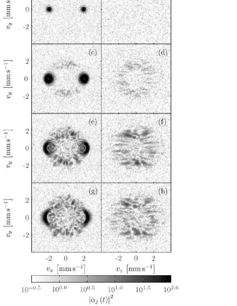
Figure 1: Velocity mode populations on the planes $v_{z}=0$ (a,c,e,g) and $v_{x}=0$ (b,d,f,h) at times $t=0$ (a,b), 8.2 ms (c,d), 16.4 ms (e,f) and 37.7 ms (g,h) for our colliding system described in the text. Note that the simulation volume exceeds that shown.

In Fig. 1 we show the mode populations for a single trajectory of our colliding system, for those modes whose velocities lie on the planes $v_{z}=0$ and $v_{x}=0$, at a sequence of times. There are two major points of interest in this figure. First, we observe from the $v_{z}=0$ planes that the original condensate wavepackets broaden and change shape from ellipsoidal to crescent shaped. Secondly, we observe the generation of a circular feature, centered at the system centre of mass velocity; this is the scattering halo that is the focus of this work. Note that the mode population scale of Fig. 1 is logarithmic, where the scale has been chosen to display the lower populations to best effect. A consequence of this is that the higher populations saturate for $\left|\alpha_{j}\right|^{2}\geq 100$, which is rather lower than the population of $3.2\times 10^{4}$ for a mode at the centre of each of the condensate packets at $t=0$.

We can see from Fig. 1 that the scattering halo first appears (in our centre of mass frame) centered at a radius slightly less than the initial central wavenumber of the individual condensate wavepackets, due to the interaction energy cost associated with creating perturbations in the field Bach2002a . As time progresses the halo broadens, largely inwards, to occupy (in the average) virtually all those modes within a certain wavenumber radius. This broadening is a consequence of scattering events between particles already present in the halo with those in one of the condensate wavepackets, or other halo particles. Both processes serve to redistribute population within the halo. In addition we note from Fig. 1 (c) that when the halo first appears there is an angular dependence, with those modes whose polar angles relative to the collision ($v_{x}$) axis are closest to $\pi/2$ having the greatest increase in population.

This anisotropy occurs despite the inherent isotropy of $s$-wave scattering, because rather than the scattering of single quantum, here we are dealing with the collective scattering of many particles in the presence of a matter-wave grating. The probability of any single scattering event is thus proportional to the overlap integral between the input and output wavefunctions, which means that modes whose momenta are either perpendicular or parallel to the direction of the grating have the largest overlap integral and hence experience the greatest growth.

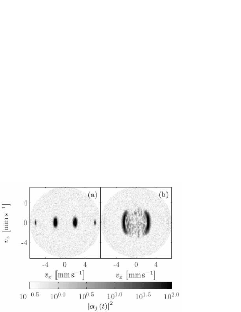
Figure 2: Single trajectory velocity mode populations on the plane $v_{y}=0$ at 1.6 ms (a) and 37.7 ms (b) for the same collision as in Fig. 1. The low-energy subspace boundary is visible as a circle, beyond which no population occurs.

Although not visible in Fig. 1, three-wave mixing between the condensate packets gives rise to additional wavepackets centered (in momentum space) at $k_{x}=\pm 3\Delta q/2$. However, due to the kinetic energy mismatch involved in their generation, these packets are transient, and have essentially disappeared by the time the initial wavepackets are separated. This effect is shown in Fig. 2, where these higher order packets are present shortly after the collision begins, and are absent by 37.7 ms. Additionally, this figure shows the asymmetry in the condensate wavepackets both initially and as a result of anisotropic broadening due to the oblate nature of the initial trapped condensate.

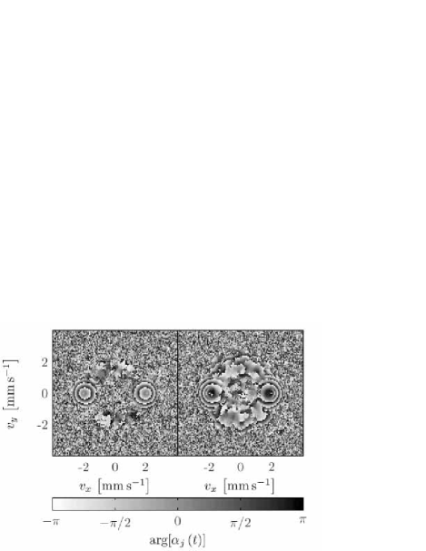
Figure 3: Single trajectory velocity mode phases on the plane $v_{z}~{}=~{}0$ at 8.2 ms (left) and 16.4 ms (right), corresponding to Fig. 1 (c,e).

The scattering halo is not uniformly populated. Rather it is characterized by distinct patches of high population separated by regions of low population. In Fig. 3 we plot the phases of the modes on the plane $v_{z}=0$ at times corresponding to the second and third rows of Fig. 1. From Fig. 3 (left) we observe that as the population in the halo begins to grow, small regions of relatively constant phase are formed, which by comparing Figs. 1 and 3 can be identified with those regions of relatively high population. Hence we label these small, highly-populated regions of momentum space phase grains. The size and aspect ratio of these phase grains is very similar to those of the initial condensate wavepackets in momentum space, a result that we explore more quantitatively in section V.5. We note that the phase profile of each grain is established prior to any significant population gain.

V.1.2 Coordinate space

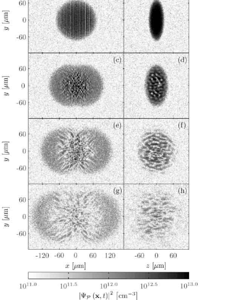
Figure 4: Coordinate space density for the same collision as Fig. 1 on the planes $z=0$ (a,c,e,g) and $x=0$ (b,d,f,h) at times $t=0$ (a,b), 12.6 ms (c,d), 25.1 ms (e,f) and 37.7 ms (g,h). Note the logarithmic density scale.

In Fig. 4 we show the evolving total coordinate space density $\left|\Psi_{\mathcal{P}}\left({\bf x},t\right)\right|^{2}$ on the planes $z=0$ and $x=0$ for the trajectory shown in the preceding section. The initial state of the field, shown by Fig. 4 (a,b), displays the modulated ground state condensate profile given by Eq. (56), while the vacuum noise component is observed to be spatially uniform in its average density, as required for the plane-wave basis, extending into and distorting the condensate profile.

As the collision proceeds we observe that at the centre of the system, where the particle density is highest, the regular fringe pattern arising from the overlapping wavepackets begins to break down, indicating that quanta are being generated with momenta other than those of the condensate wavepackets. By 25.1 ms into the collision, as shown in Fig. 4 (e), the fringes appear to be completely absent. Following this breakdown, the high density region of the field comprises two distinct types of wavefunction, a relatively smooth outer portion and a fragmented central region. In section V.2, we identify the smooth outer shells as condensate that survives the collision, while the central region forms the scattered halo, together with a very small condensate remnant. The highest density during the course of the simulation remains close to the origin, which somewhat counterintuitively leads to the scattered quanta being more dense than the condensates at later times. After separation of the condensate packets, scattering events taking place within the central (fragmented) region involve at most one condensate quantum, and redistribute population within the halo.

Estimating the separation time using Thomas-Fermi condensate wavepackets of unchanging shape returns 30.6 ms, significantly longer than that observed in our simulation. The reduction in separation time reflects the significantly distorted condensate packets, from initially ellipsoidal to a shape most easily described as a hemi-ellipsoidal shell (see Fig. 4 (g)).

We observe from Fig. 4 (g) that near the end of the simulation, the coordinate space field is beginning to resemble the momentum space field, as shown by Fig. 1 (g). By this time the rate of change of the mode populations is very small, and we therefore expect that Fig. 1 (g) will give an excellent indication of the coordinate space density distribution for the system following a sufficiently long ballistic expansion.

V.1.3 Turbulence

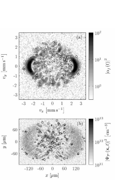
Figure 5: (a) Velocity mode populations on the plane $v_{z}=0$ and (b) coordinate space density on the plane $z=0$ at 37.7 ms into the collision. Crosses and circles respectively show unit vortices of positive and negative sense.

Within the scattering halo, a large number of vortices have been detected between the highly populated grains in both velocity and coordinate spaces. We demonstrate this in Fig. 5, where we show the velocity mode populations on the plane $v_{z}=0$ and the coordinate space density on the plane $z=0$ at the end of the collision, together with the detected vortices. Note that we plot in Fig. 5 only those vortices that reside in regions of relatively high average mode population ($\mathcal{N}_{j}>1$) or density ($\left|\Psi_{\mathcal{P}}\right|^{2}>3\times 10^{11}$ cm^-3), which filters out those vortices that are present in the field solely by the presence of the virtual particle fluctuations, and those that are physically observable, although the threshold choice is somewhat arbitrary.

We have observed (but not plotted) that a significant growth in the number of physical vortices coincides with the growth of the scattering halo, indicating that, in much the same way as the halo growth can be viewed as amplification of the vacuum fluctuations, the observed vortices are amplifications of the underlying quantum vortices. This provides the basis for our identification of quantum turbulence within the scattering halo.

V.2 Coherent and incoherent fields

We have assembled an ensemble of 80 individual trajectories of our colliding system, where the initial states of each differ only in the applied virtual particle noise, as described in section II.3.2. In the following sections we use this ensemble to calculate various quantum statistics of the colliding system.

V.2.1 Momentum space

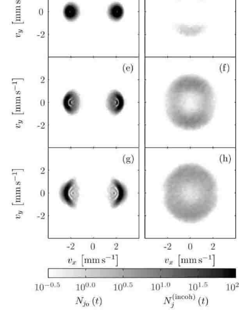
Figure 6: Coherent (a,c,e,g) and incoherent (b,d,f,h) velocity mode populations on the plane $v_{z}~{}=~{}0$ at times 0 (a,b), 8.2 ms (c,d), 16.4 ms (e,f) and 37.7 ms (g,h).

Using the correspondence between moments of the Wigner function and symmetrized operator products, Eq. (17), we can calculate the total expectation population of the $j$th mode, $N_{j}\left(t\right)$, using

$$N_{j}\left(t\right)\equiv\left\langle\hat{N}_{j}\right\rangle\left(t\right)=\left\langle\hat{a}_{j}^{\dagger}\hat{a}_{j}\right\rangle\left(t\right)=\left\langle\left|\alpha_{j}\left(t\right)\right|^{2}\right\rangle_{W}-\frac{1}{2}.$$ (59)

Using the coherent amplitude of the $j$th mode

$$\alpha_{j_{0}}\left(t\right)\equiv\left\langle\hat{a}_{j}\right\rangle\left(t\right)=\left\langle\alpha_{j}\left(t\right)\right\rangle_{W},$$ (60)

we can calculate the coherent (i.e. condensate) part of the total mode population as

$$N_{j_{0}}\left(t\right)\equiv\left|\left\langle\alpha_{j}\left(t\right)\right\rangle_{W}\right|^{2}.$$ (61)

In Fig. 6 (a,c,e,g) we plot the coherent mode populations on the plane $v_{z}=0$ for our colliding system. From these plots we observe that the condensate population is restricted to two wavepackets that, consistent with the behavior shown in Fig. 1, broaden and change shape over the course of the collision. A benefit of plotting the coherent populations only is that the small-scale structure of the condensate packets is rather more apparent here than in Fig. 1. Although not shown in Fig. 6, the higher order wavepackets, when they appear, are also found to contain condensate particles.

The corresponding incoherent mode populations are calculated as the difference

$$N_{j}^{\left({\rm incoh}\right)}\left(t\right)\equiv N_{j}\left(t\right)-N_{j_{0}}\left(t\right).$$ (62)

In Fig. 6 (b,d,f,h) we plot the incoherent mode populations on the plane $v_{z}=0$ for the collision. From these plots we observe that from an initial state with zero incoherent population (as required by our assumed initial Wigner function), incoherent population builds up initially as a semi-spherical scattering halo, where those modes occupied by the condensate wavepackets have a relatively small incoherent population. Subsequently population is transferred, via further scattering events, to broaden the distribution of incoherent quanta.

V.2.2 Coordinate space

The coherent and incoherent fields can also be calculated in coordinate space. Using the coherent probability amplitude

$$\Psi_{\mathcal{P}_{0}}\left({\bf x},t\right)\equiv\left\langle\hat{\Psi}_{\mathcal{P}}\left({\bf x}\right)\right\rangle\left(t\right)=\left\langle\Psi_{\mathcal{P}}\left({\bf x},t\right)\right\rangle_{W},$$ (63)

the coherent particle density (condensate density) can be calculated as

$$n_{0}\left({\bf x},t\right)=\left|\Psi_{\mathcal{P}_{0}}\left({\bf x},t\right)\right|^{2}=\left|\sum_{j\in L}\psi_{j}\left({\bf x}\right)\alpha_{j_{0}}\left(t\right)\right|^{2}.$$ (64)

The corresponding incoherent particle density is found using both the total particle density, Eqs. (32,33), and the coherent particle density to be

$$n^{\left({\rm incoh}\right)}\left({\bf x},t\right) \equiv n\left({\bf x},t\right)-n_{0}\left({\bf x},t\right)$$ (66)

$$= \left\langle\left|\Psi_{\mathcal{P}}\left({\bf x},t\right)\right|^{2}\right\rangle_{W}-\left|\left\langle\Psi_{\mathcal{P}}\left({\bf x},t\right)\right\rangle_{W}\right|^{2}$$

$$\hskip 28.45274pt\mbox{}-\frac{1}{2}\delta_{\mathcal{P}}\left({\bf x,x}\right),$$

where the restricted delta function, $\delta_{\mathcal{P}}\left({\bf x,x}^{\prime}\right)$ is defined by Eq. (12). We plot both the coherent and incoherent particle densities for our colliding system in Fig. 7.

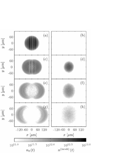
Figure 7: Coherent (a,c,e,g) and incoherent (b,d,f,h) particle densities for our colliding system on the plane $z~{}=~{}0$ at times 0 (a,b), 12.6 ms (c,d), 25.1 ms (e,f) and 37.7 ms (g,h).

From Fig. 7 (a,b) we observe that the initial state is uniformly coherent, consistent with the assumed initial Wigner function. As the collision progresses we observe that significant incoherent particle density develops close to the origin, generated from the condensate particles. Note that Fig. 7 (e,g) shows that a small interference pattern exists in this central region even late into the collision, which was not apparent from a single trajectory (see Fig. 4).

V.2.3 Total coherent and incoherent populations

One of the important quantities that can be calculated from these simulated collisions is the total number of particles scattered out of the condensate wavepackets. In our previous Letter Norrie2005a we calculated this quantity approximately using a spatially dependent counting method in momentum space. Such methods are routinely used experimentally. However, using our ensemble we can obtain the total coherent population

$$N_{0}\left(t\right)\equiv\sum_{j\in L}\left|\alpha_{j_{0}}\left(t\right)\right|^{2},$$ (67)

and incoherent population

$$N^{\left({\rm incoh}\right)}\left(t\right)\equiv N-N_{0}\left(t\right),$$ (68)

with a great deal more accuracy.

A well-known result for averages of randomly distributed variables is that the convergence of a finite number of samples $\mathcal{M}$ to the true value scales as $1/\sqrt{\mathcal{M}}$ (where convergence is measured as the error in the calculated average). We define the total coherent field population, calculated from $\mathcal{M}$ trajectories, as

$$N_{0}\left(t\right)^{\left(\mathcal{M}\right)}\equiv\sum_{j\in L}\left|\frac{1}{\mathcal{M}}\sum_{m=1}^{\mathcal{M}}\alpha_{j}\left(t\right)^{\left(m\right)}\right|^{2},$$ (69)

where $\alpha_{j}\left(t\right)^{\left(m\right)}$ is the time-dependent mode amplitude of the $m$th trajectory. Given the large number of modes within our colliding system, and the magnitude squaring operation in Eq. (69), it is expected that

$$N_{0}\left(t\right)^{\left(\mathcal{M}\right)}\approx N_{0}\left(t\right)+\frac{C\left(t\right)}{\mathcal{M}},$$ (70)

where $N_{0}\left(t\right)=N_{0}\left(t\right)^{\left(\infty\right)}$. Here $C\left(t\right)$ is some dimensionless time-dependent function, independent of $\mathcal{M}$, whose exact form is in fact unimportant for our purposes. Assuming that Eq. (70) holds, we can therefore use any two calculated $N_{0}\left(t\right)^{\left(\mathcal{M}\right)}$ of dissimilar $\mathcal{M}$ to obtain the ensemble limit. In particular, using $\mathcal{M}=1$ for one of these two, we find that

$$N_{0}\left(t\right)\approx\frac{N_{0}\left(t\right)^{\left(1\right)}-\mathcal{M}N_{0}\left(t\right)^{\mathcal{M}}}{1-\mathcal{M}}.$$ (71)

In practise we find that this extrapolation method is extremely accurate using just two trajectories. This result makes a survey of the parameter dependence of the global field quantities numerically efficient although, unfortunately, an equivalent extrapolation method for local field quantities is significantly less accurate.

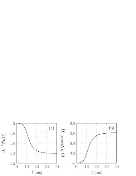
Figure 8: Total coherent (a) and incoherent (b) populations for the colliding system calculated using the extrapolation method outlined in the text.

In Fig. 8 we plot the total coherent and incoherent populations for our colliding system, calculated using our extrapolation method with $\mathcal{M}=80$. From these curves we observe that the coherent population monotonically decreases with time, with the most significant depletion occurring between 5 ms and 25 ms into the collision, by which time 30% of the total population is incoherent. Note that the incoherent population continues to increase even after separation of the condensate wavepackets, which results from decohering interactions involving individual wavepackets only. Note also that the difference in the calculated populations is less than 1.5% for all $\mathcal{M}\in\left[2,80\right]$.

V.3 Local correlation functions

V.3.1 Momentum space

The normalized second-order equiposition mode-space correlation function

$$g_{j}^{\left(2\right)}\left(t\right)\equiv\frac{\left\langle\hat{a}_{j}^{\dagger}\hat{a}_{j}^{\dagger}\hat{a}_{j}\hat{a}_{j}\right\rangle\left(t\right)}{\left[\left\langle\hat{a}_{j}^{\dagger}\hat{a}_{j}\right\rangle\left(t\right)\right]^{2}},$$ (72)

probes the quantum statistics of the $j$th momentum mode. If a mode displays coherent statistics, then we should observe that $g_{j}^{\left(2\right)}=1$. Conversely, if the mode displays Gaussian (i.e. thermal) statistics, then we should find that $g_{j}^{\left(2\right)}=2$. By applying the correspondence of the Wigner function moments to the symmetrized quantum expectation values, Eq. (17), we find that $g_{j}^{\left(2\right)}\left(t\right)$ can be calculated using

$$g_{j}^{\left(2\right)}\left(t\right)=\frac{\left\langle\left|\alpha_{j}\left(t\right)\right|^{4}\right\rangle_{W}-2\left\langle\left|\alpha_{j}\left(t\right)\right|^{2}\right\rangle_{W}+\frac{1}{2}}{\left[\left\langle\left|\alpha_{j}\left(t\right)\right|^{2}\right\rangle_{W}-\frac{1}{2}\right]^{2}}.$$ (73)

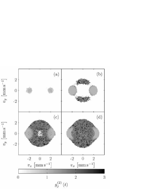
Figure 9: Normalized second-order mode space correlation function $g^{\left(2\right)}_{j}\left(t\right)$ for the colliding system, on the plane $v_{z}~{}=~{}0$, at times 0 (a), 8.2 ms (b), 16.4 ms (c) and 37.7 ms (d). Results are only shown for those modes with $N_{j}>1/2$.

We plot $g_{j}^{\left(2\right)}\left(t\right)$ on the plane $v_{z}=0$ for our colliding system in Fig. 9. Due to the normalized character of the correlation function and the finite number of ensemble members, those modes with small populations give highly noisy results. Therefore we have plotted in Fig. 9 only those modes whose real particle population is larger than one half. (Of course the quantum statistics of a mode are only defined when that mode is populated.) From Fig. 9 we observe that the condensate wavepackets have $g_{j}^{\left(2\right)}=1$, and are therefore coherently populated, whereas the halo modes have $g_{j}^{\left(2\right)}\approx 2$, characteristic of Gaussian statistics. The higher level of noise in the results returned for the halo modes as opposed to the condensate modes is a consequence of the much lower average population of the halo modes, and would be reduced for an increased number of ensemble members.

V.3.2 Coordinate space

We can similarly characterize the quantum statistics of the system in coordinate space, for which the appropriate analogue to Eq. (72) is

$$g^{\left(2\right)}\left({\bf x},t\right)\equiv\frac{\left\langle\hat{\Psi}_{\mathcal{P}}^{\dagger}\left({\bf x}\right)\hat{\Psi}_{\mathcal{P}}^{\dagger}\left({\bf x}\right)\hat{\Psi}_{\mathcal{P}}\left({\bf x}\right)\hat{\Psi}_{\mathcal{P}}\left({\bf x}\right)\right\rangle\left(t\right)}{\left[\left\langle\hat{\Psi}_{\mathcal{P}}^{\dagger}\left({\bf x}\right)\hat{\Psi}_{\mathcal{P}}\left({\bf x}\right)\right\rangle\left(t\right)\right]^{2}}.$$ (74)

By expanding the field operators on the restricted mode basis, Eq. (3) and applying the Wigner function moment correspondences, Eq. (17), we find that the second order normalized coordinate space correlation function can be calculated using

$$g^{\left(2\right)}\left({\bf x},t\right)=\frac{\left\langle\left|\Psi_{\mathcal{P}}\right|^{4}\right\rangle_{W}-2\left\langle\left|\Psi_{\mathcal{P}}\right|^{2}\right\rangle_{W}\delta_{\mathcal{P}}+\frac{1}{2}\delta_{\mathcal{P}}^{2}}{\left[\left\langle\left|\Psi_{\mathcal{P}}\right|^{2}\right\rangle_{W}-\frac{1}{2}\delta_{\mathcal{P}}\right]^{2}},$$ (75)

where for conciseness we have written $\Psi_{\mathcal{P}}=\Psi_{\mathcal{P}}\left({\bf x},t\right)$ and $\delta_{\mathcal{P}}=\delta_{\mathcal{P}}\left({\bf x,x}\right)$. As with $g^{\left(2\right)}_{j}\left(t\right)$, Eq. (75) should return unity for regions of coherently distributed density and two for regions of Gaussian distributed density.

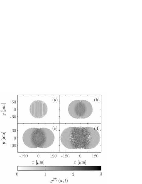
Figure 10: Normalized second-order equiposition coordinate space correlation function $g^{\left(2\right)}\left({\bf x},t\right)$ for the collision on the plane $z~{}=~{}0$ at times 0 (a), 12.6 ms (b), 25.1 ms (c) and 37.7 ms (d). Results are only shown for those points where $n\left({\bf x}\right)>3\times 10^{11}$ cm^-3.

In Fig. 10 we plot $g^{\left(2\right)}\left({\bf x},t\right)$ for the collision, calculated using Eq. (75), at a sequence of times. These plots again show a uniformly coherent initial state, as required, and as time progresses we observe that close to the centre of the collision the system becomes increasing incoherent, reflecting the creation of the halo, so that by 37.7 ms the central region shows $g^{\left(2\right)}\left({\bf x},t\right)\sim 2$.

V.4 Pair creation correlation functions

The halo formation process can be viewed as a four-wave mixing, in which the two input particles are from each of the condensate wavepackets, and the output particles appear (in the centre of mass frame) in modes of approximately (due to the finite momentum spread of the condensate wavepackets) opposite momentum. It is expected therefore that modes of opposite momenta will display correlations in both their amplitude and population, at least at early times.

An appropriate (normalized) correlation function to quantify the amplitude correlation between modes of opposing momenta is

$$g^{\left(0,2\right)}_{ij}\left(t\right)\equiv\frac{\left\langle\hat{a}_{i}\hat{a}_{j}\right\rangle\left(t\right)-\left\langle\hat{a}_{i}\right\rangle\left(t\right)\left\langle\hat{a}_{j}\right\rangle\left(t\right)}{\sqrt{\left\langle\hat{a}^{\dagger}_{i}\hat{a}_{i}\right\rangle\left(t\right)\left\langle\hat{a}_{j}^{\dagger}\hat{a}_{j}\right\rangle\left(t\right)}},$$ (76)

where we use ${\bf k}_{j}=-{\bf k}_{i}$ and the second term in the numerator corrects for the non-zero amplitude expectation value for condensate modes. This function can be written in terms of moments of the Wigner function as

$$g^{\left(0,2\right)}_{ij}\left(t\right)=\frac{\left\langle\alpha_{i}\left(t\right)\alpha_{j}\left(t\right)\right\rangle_{W}-\left\langle\alpha_{i}\left(t\right)\right\rangle_{W}\left\langle\alpha_{j}\left(t\right)\right\rangle_{W}}{\sqrt{\left[\left\langle\left|\alpha_{i}\left(t\right)\right|^{2}\right\rangle_{W}-\frac{1}{2}\right]\left[\left\langle\left|\alpha_{j}\left(t\right)\right|^{2}\right\rangle_{W}-\frac{1}{2}\right]}}.$$ (77)

We plot the magnitude of $g^{\left(0,2\right)}_{ij}\left(t\right)$ for ${\bf k}_{j}=-{\bf k}_{i}$ at a sequence of times in Fig. 11. (Due to our choice of $i,j$ momenta the results are symmetric about the origin.) From these slices we observe that there is a definite amplitude correlation between modes of opposite momenta, largest at early times ($g^{\left(0,2\right)}_{ij}\left(t\right)\sim 0.3$ at 6.6 ms), and decreasing as the collision progresses. The degradation in the correlation as time progresses is a consequence of the subsequent scattering events, which leads to the correlation between paired modes becoming essentially zero at late times.

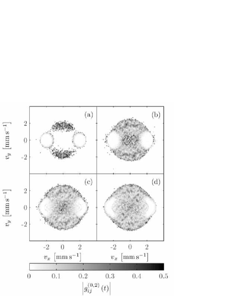
Figure 11: Magnitude of the mode amplitude pair creation correlation function $g^{\left(0,2\right)}_{ij}\left(t\right)$ on the plane $v_{z}~{}=~{}0$ at 6.6 ms (a), 13.1 ms (b), 19.7 ms (c) and 37.7 ms (d). Results are only shown for those modes with $N_{j}>1/4$.

Note that in Fig. 11 we have only plotted results for which $N_{j}>1/4$. Although we can calculate the correlation function for all modes and at all times, the results have no physical meaning for unpopulated modes. Furthermore, modes with very low population produce very noisy results.

The analogue to Eq. (76) for measuring the population correlation between paired modes is

$$g^{\left(2\right)}_{ij}\left(t\right)\equiv\frac{\left\langle\hat{a}_{i}^{\dagger}\hat{a}_{j}^{\dagger}\hat{a}_{i}\hat{a}_{j}\right\rangle\left(t\right)}{\left\langle\hat{a}^{\dagger}_{i}\hat{a}_{i}\right\rangle\left(t\right)\left\langle\hat{a}_{j}^{\dagger}\hat{a}_{j}\right\rangle\left(t\right)}.$$ (78)

We have calculated this quantity, and have observed essentially the same behavior as for the amplitude correlations, i.e. a definite correlation exists at early times, that decreases rapidly with time. We note however that a very large error exists in the calculations of $g^{\left(2\right)}_{ij}$ (of order $\pm 2$ at $t=6$ ms), much larger than for the amplitude correlations, so that quantifying the degree of this correlation is difficult.

V.5 Autocorrelation function

As shown by Figs. 1, 2 and 3, the scattering halo in momentum space is characterized by discrete phase grains. To quantify the size of these grains, and hence the range of phase order within the halo, we use the normalized autocorrelation function

$$g^{\left(1\right)}_{ij}\left(t\right)\equiv\frac{\left\langle\hat{a}_{i}^{\dagger}\hat{a}_{j}\right\rangle\left(t\right)}{\sqrt{\left\langle\hat{a}_{i}^{\dagger}\hat{a}_{i}\right\rangle\left(t\right)\left\langle\hat{a}_{j}^{\dagger}\hat{a}_{j}\right\rangle\left(t\right)}},$$ (79)

which in terms of moments of the Wigner function is

$$g^{\left(1\right)}_{ij}\left(t\right)=\frac{\left\langle\alpha_{i}^{*}\left(t\right)\alpha_{j}\left(t\right)\right\rangle_{W}-\frac{1}{2}\delta_{i,j}}{\sqrt{\left[\left\langle\left|\alpha_{i}\left(t\right)\right|^{2}\right\rangle_{W}-\frac{1}{2}\right]\left[\left\langle\left|\alpha_{j}\left(t\right)\right|^{2}\right\rangle_{W}-\frac{1}{2}\right]}}.$$ (80)

Although modes $i$ and $j$ can be arbitrarily chosen, for this analysis we fix mode $i$ at ${\bf v}_{i}=\left(0,1.8~{}{\rm mm\,s}^{-1},1\right)$ and vary $j$ over the full mode space, for which the autocorrelation function is shown on the planes $v_{z}=0$ and $v_{x}=0$ in Fig. 12. From these plots we observe that the significant feature of the autocorrelation function is a small ellipsoid, visible as a black grain centered on ${\bf v}_{j}={\bf v}_{i}$, whose size and shape remains relatively unchanged through time.

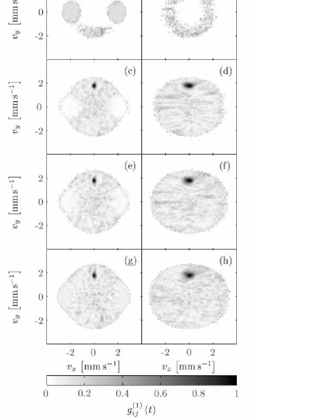
Figure 12: Normalized mode space autocorrelation function $g^{\left(1\right)}_{ij}\left(t\right)$ on the planes $v_{z}=0$ (a,c,e,g) and $v_{x}=0$ (b,d,f,h) at 6.6 ms (a,b), 13.1 ms (c,d), 19.7 ms (e,f) and 37.7 ms (g,h). Here ${\bf v}_{i}=(0,1.8~{}{\rm mm\,s}^{-1},0)$ and results are only shown for modes with $N_{j}>1/4$.

To more precisely quantify the time-dependent shape of this grain we have fitted a three-dimensional Gaussian profile to the correlation function, over a region of approximately the same extent as the grain. At the time when significant population is first established in the halo (8 ms), the HWFM widths of the fitted Gaussian are approximately 0.3 mm s^-1, 0.3 mm s^-1 and 0.8 mm s^-1 in the $v_{x}$, $v_{y}$ and $v_{z}$ directions respectively. These widths reflect the asymmetry of the initial condensate wavepackets (in velocity space), and are approximately 1.5 times as large as the velocity radii of the condensate wavepackets in the Thomas-Fermi approximation (being 0.19 mm s^-1 in the $v_{x}$ and $v_{y}$ directions and 0.54 mm s^-1 in the $v_{z}$ direction). At later times, the fitted widths are found to increase anisotropically, so that by 40 ms the fitted widths are approximately 0.3 mm s^-1, 0.6 mm s^-1 and 0.9 mm s^-1. These increases are driven by scattering events, and reflect the inverse extent of the colliding system in coordinate space (see Fig. 4).

V.6 Parameter dependence

In this section we explore the dependence of the coherent and incoherent populations on the initial condensate number and on the initial relative wavepacket speed. These parameters, which are relatively easily adjusted experimentally, are the only ones we change — all other simulation parameters, including $U_{0}$, $\omega_{x,y,z}$ and the details of the simulation grids, are held fixed. We obtain the time-dependent total coherent and incoherent populations for each parameter set using the extrapolation method outlined in section V.2.3. For all parameter sets two trajectories were simulated.

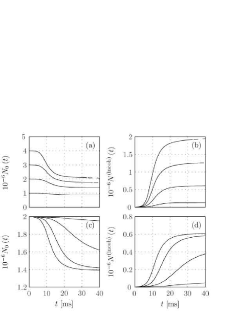
Figure 13: Total coherent and incoherent populations calculated using the extrapolation method for varying collision parameters. Plots (a,b) show (respectively) the coherent and incoherent populations for collisions with $\Delta v=4.0$ mm s^-1 with (lowest to highest) $N_{0}\left(t=0\right)=\left\{1,2,3,4\right\}\times 10^{6}$. Plots (c,d) show the coherent and incoherent populations for collisions with $N_{0}\left(t=0\right)=2\times 10^{6}$ and (highest to lowest in (c) and lowest to highest in (d)) $\Delta v=\left\{1.0,2.0,3.0,4.0\right\}$ mm s^-1.

V.7 Initial condensate number

In Fig. 13 (a,b) we plot the total coherent and incoherent populations for collisions at $\Delta v=4.0$ mm s^-1 with total initial condensate numbers of $N_{0}\left(t=0\right)=\left\{1,2,3,4\right\}\times 10^{6}$. From these curves we can see that by increasing the total number of particles within the system, the amount of incoherent population generated by the collision also increases. We find that the peak rate of incoherent particle formation increases roughly linearly with $N_{0}\left(0\right)$, and that the time that this peak occurs decreases, with increasing particle number. The dashed parts of the curves for $N_{0}\left(t=0\right)=\left\{3,4\right\}\times 10^{6}$ indicate results where the real particle density has begun to exit the simulation volume.

V.8 Collision speed

In Fig. 13 (c,d) we plot the total coherent and incoherent populations for collisions with $N_{0}\left(t=0\right)=2\times 10^{6}$ and $\Delta v=\left\{1.0,2.0,3.0,4.0\right\}$ mm s^-1. These curves show that the rate of incoherent population scattering increases (again found to be roughly linearly) with increasing relative wavepacket speed, a result which is expected from classical collisional theory $\left(n\sigma v\right)$. However, as can be seen for the curves with $\Delta v=\left\{3.0,4.0\right\}$ mm s^-1, the total amount of incoherent population generated is less strongly dependent upon $\Delta v$, as the overlap time of the condensate wavepackets, and hence the period over which the major mechanism of incoherent particle formation acts, scales as $\approx 1/\sqrt{\Delta v}$. For the lower values of $\Delta v$, broadening of the condensate wavepackets leads to the population exiting the simulation volume before packet separation. Note that the the speed of sound for this system (taken as for a homogeneous system at the peak density of the condensate at $t=0$) is 1.5 mm s^-1.

V.9 The halo formation process

The basic mechanism of halo formation is pairwise scattering of condensate particles into two distinct halo modes, which can be viewed as a four-wave mixing process. However, not all modes within the halo region exhibit population growth, a feature that can be understood in terms of the phase relationships required for growth. For plane wave modes, the nonlinear portion of the mode amplitude evolution is

$$i\frac{d\alpha_{j}}{dt}^{\left({\rm nonlin}\right)}=\frac{U_{0}}{V}\sum_{rst\in L}\alpha_{r}^{*}\alpha_{s}\alpha_{t}\delta_{{\bf k}_{j}+{\bf k}_{r},{\bf k}_{s}+{\bf k}_{t}},$$ (81)

representing a process where $s+t\rightarrow j+r$. Writing the mode amplitudes as $\alpha_{j}\left(t\right)=\sqrt{\mathcal{N}_{j}}\exp\left[i\theta_{j}\left(t\right)\right]$, the rate of population change for a single mode (in the absence of external potentials) is

$$\frac{d\mathcal{N}_{j}}{dt}=-\frac{2U_{0}}{V}\sum_{rst\in L}\sqrt{\mathcal{N}_{j}\mathcal{N}_{r}\mathcal{N}_{s}\mathcal{N}_{t}}\sin\left(\Theta_{jrst}\right)\delta_{\mathbf{k}_{j}+\mathbf{k}_{r},\mathbf{k}_{s}+\mathbf{k}_{t}},$$ (82)

where $\Theta_{jrst}\equiv\theta_{j}+\theta_{r}-\theta_{s}-\theta_{t}$. The phase evolution corresponding to Eq. (82) is

$$\frac{d\theta_{j}}{dt}=-\frac{U_{0}}{V}\sum_{rst\in L}\sqrt{\frac{\mathcal{N}_{r}\mathcal{N}_{s}\mathcal{N}_{t}}{\mathcal{N}_{j}}}\cos\left(\Theta_{jrst}\right)\delta_{\mathbf{k}_{j}+\mathbf{k}_{r},\mathbf{k}_{s}+\mathbf{k}_{t}}.$$ (83)

At early times, the evolution of the halo modes is driven almost entirely by the condensate wavepackets, with the dominant processes being scattering events involving the destruction of one quanta from each wavepacket. The role of the phase $\Theta_{jrst}$ is critical, as can be understood from a simplified model of four modes only, two highly occupied modes $s$ and $t$ representing the two condensate packets, and a pair of scattered modes $j$ and $r$ of lower occupation, for which $\mathbf{k}_{r}=-\mathbf{k}_{j}$ (in the centre of mass frame). Initially the phase $\Theta_{jrst}$ is randomly set, and if $-\pi<\Theta_{jrst}<0$, population transfers from the pair $(s,t)$ into the pair $(j,r),$ while if $0<\Theta_{jrst}<\pi,$ the population transfer is in the opposite direction. The phase $\Theta_{jrst}$ evolves towards either $-\pi/2$ (maximum gain for scattered modes) or $+\pi/2$ (maximum loss), where it stabilizes while population is still available for transfer. Thus some pairs $(j,r)$ will grow, while others will decrease in size. If $\mathcal{N}_{j}\ll\mathcal{N}_{r}$, the phase $\theta_{j}$ can change rapidly (see Eq. (83)), possibly leading to a change in the direction of population transfer.

For the multimode case, the main additional feature is that the scattered modes no longer need be precise momentum opposites, because of the range of momentum modes available in the condensate packets. Thus for a particular scattered mode $j$ there is a range of possible modes near its conjugate momentum mode $r$ which can be convolved with the condensate packets to contribute to the growth (or loss) in $j$, (see Eq. (81)). Labelling this set of modes about $r$ as $R$, then from the properties of convolution, the size of $R$ is about twice that of a condensate packet. There is of course a corresponding set of modes $J$ about $j$, and if the phases and populations for a pair of modes from $R$ and $J$ are favorable for growth, these phases can quickly be locked across the regions $R$ and $J$ (see Fig  3). Population growth is a stimulated process, so while $R$ and $J$ will now grow rapidly, regions which have not established a favorable phase are left behind.

We note that this discussion helps explain the incomplete pair correlation observed for halo modes $j$ and $r$, because the scattered pair are not required to have exactly opposite momentum, due to the range of momentum modes available in the condensate packets.

VI Conclusion

In this paper we have presented a complete derivation of the truncated Wigner method, paying particular attention to the limits of validity of the Wigner truncation. Using this formalism, we have presented simulation results, both from a single trajectory and from ensembles of trajectories, of collisions between distinct Bose-Einstein condensate wavepackets. This formalism includes both stimulated and spontaneous processes, allowing for a complete treatment of system dynamics. In particular we have observed the generation of highly populated $s$-wave scattering haloes. Previous treatments of similar collisional systems have been restricted to the low-scattering limit, and have not provided a complete description of the field.

The most significant process not included in our treatment of these collisions is three-body recombination Wieman1997a . In a further paper Norrie2005c we extend the truncated Wigner method to include this process, and investigate its effect on a simple system. For the colliding systems considered in this paper we have found using this extended formalism that three-body recombination has a negligible effect on the dynamics.

VI.1 Relationship to the projected Gross-Pitaevskii equation

The various forms of the truncated Wigner differential equation, Eqs. (36,37,38), are functionally identical to the Projected Gross-Pitaevskii equation of Davis et al. Davis2001a ; Davis2001b ; Davis2002a . However the projected Gross-Pitaevskii equation treatment has been used only for relatively high temperature situations, in which the thermal fluctuations are much larger than the quantum fluctuations, whereas in the truncated Wigner method the quantum mechanical nature of the system is still largely present in the form of mode amplitude fluctuations in the initial state (see below). The initial state of the Gross-Pitaevskii equation system would represent the limit, in the truncated Wigner function method, in which the size of the quantum fluctuations becomes negligible in comparison with the size of the order parameter of the field, while keeping the number of particles in the field constant. Thus the Gross-Pitaevskii equation can be considered to represent the thermodynamic limit of the truncated Wigner approach where spontaneous, and spontaneously initiated, processes are far less important than stimulated processes. Of course the alternate approach is then simply to take the Gross-Pitaevskii equation, and “seed” each mode with a certain amount of noise, such that previously unavailable spontaneous processes become possible. While this approach would avoid some of the more complicated aspects of the truncated Wigner method, one could not then make the unambiguous connections to the underlying quantum nature of the system which the truncated Wigner method allows.

References

- (1) A. P. Chikkatur et al., Phys. Rev. Lett. 85, 483 (2000).
- (2) N. Katz, J. Steinhauer, R. Ozeri, and N. Davidson, Phys. Rev. Lett. 89, 220401 (2002).
- (3) J. M. Vogels, K. Xu, and W. Ketterle, Phys. Rev. Lett. 89, 020401 (2002).
- (4) Y. B. Band, M. Trippenbach, J. J. P. Burke, and P. S. Julienne, Phys. Rev. Lett. 84, 5462 (2000).
- (5) R. Bach, M. Trippenbach, and K. Rza̧żewski, Phys. Rev. A 65, 063605 (2002).
- (6) V. A. Yurovsky, Phys. Rev. A. 65, 033605 (2002).
- (7) A. A. Norrie, R. J. Ballagh, and C. W. Gardiner, Phys. Rev. Lett. 94, 040401 (2005).
- (8) E. Braaten and A. Nieto, Eur. Phys. J. B11, 143 (1999) [cond-mat/9707199].
- (9) J. O. Andersen, Rev. Mod. Phys. 76, 599 (2004).
- (10) M. J. Steel et al., Phys. Rev. A 58, 4824 (1998).
- (11) P. Deuar and P. D. Drummond, J. Phys. A: Math. Gen. 39 1163 (2006)
- (12) P. Deuar and P. D. Drummond, cond-mat/0501058 (2005)
- (13) H. T. C. Stoof, J. Low Temp. Phys. 114, 11 (1999).
- (14) R. A. Duine and H. T. C. Stoof, Phys. Rev. A 65, 013603 (2001).
- (15) H. T. C. Stoof and M. J. Bijlsma, J. Low Temp. Physics 124, 431 (2001).
- (16) M. J. Davis, R. J. Ballagh, and K. Burnett, J. Phys. B 34, 4487 (2001).
- (17) M. J. Davis, S. A. Morgan, and K. Burnett, Phys. Rev. Lett. 87, 160402 (2001).
- (18) A. Sinatra, C. Lobo, and Y. Castin, Phys. Rev. Lett. 87, 210404 (2001).
- (19) K. Gòral, M. Gajda, and K. Rza̧żewski, Opt. Express 8, 92 (2001).
- (20) C. W. Gardiner, J. R. Anglin, and T. I. A. Fudge, J. Phys. B 35, 1555 (2002).
- (21) M. J. Davis, S. A. Morgan, and K. Burnett, Phys. Rev. A 66, 053618 (2002).
- (22) K. Góral, M. Gajda, and K. Rza̧żewski, Phys. Rev. A 66, 051602(R) (2002).
- (23) H. Schmidt et al., J. Opt. B 5, 96 (2003).
- (24) N. Katz, E. Rowen, R. Ozeri and N. Davidson, Phys. Rev. Lett. 95, 220403 (2005)
- (25) P. D. Drummond and J. F. Corney, Phys. Rev. A 60, R2661 (1999).
- (26) C. W. Gardiner and P. Zoller, Quantum Noise, 3rd ed. (Springer-Verlag, Berlin, 2004).
- (27) S. A. Morgan, J. Phys. B 33, 3847 (2000).
- (28) A. Polkovnikov, Phys. Rev. A 68, 053604 (2003).
- (29) A. Sinatra, C. Lobo, and Y. Castin, J. Phys. B 35, 3599 (2002).
- (30) C. W. Gardiner, Handbook of Stochastic Methods, 3rd ed. (Springer-Verlag, Berlin, 2004).
- (31) R. J. Ballagh, Computational methods for nonlinear partial differential equations, http://www.physics.otago.ac.nz/research/uca/resources/comp_lectures_ballagh.html, 2000.
- (32) W. H. Press, S. A. Teukolsky, W. T. Vetterling, and B. P. Flannery, Numerical Recipes in C, 2nd ed. (Cambridge University Press, Cambridge, MA, 1992).
- (33) J. M. Vogels, K. Xu, and W. Ketterle, Phys. Rev. Lett. 89, 020401 (2002).
- (34) M. Kozuma et al., Phys. Rev. Lett. 82, 871 (1999).
- (35) F. Dalfovo, S. Giorgini, L. P. Pitaevskii, and S. Stringari, Rev. Mod. Phys. 71, 463 (1999).
- (36) S. A. Morgan, A Gapless Theory of Bose-Einstein Condensation in Dilute Gases at Finite Temperatures, DPhil Thesis, University of Oxford, 1999.
- (37) E. A. Burt et al., Phys. Rev. Lett. 79, 337 (1997).
- (38) A. A. Norrie, R. J. Ballagh, C. W. Gardiner, and A. S. Bradley, Submitted.