Electron transmission between normal and heavy electron metallic phases in Kondo lattices

Abstract

The interface between a heavy fermion metallic phase and a “normal” (light-fermion) metal phase is discussed. The Fermi momentum mismatch between the two phases causes the carriers to scatter at the interface. The interface conductance is a monotonous increasing function of conduction electron density, $n_{c}$, and is almost 60% of that of a clean heavy fermion metal at half-filling ($n_{c}=1$) and can be measured experimentally. Interface experiments can be used as probe of the nature of the homogenous heavy-fermion state and provide important information on the effects of inhomogeneities in heavy-fermion alloys.

I Introduction

In Kondo lattice metals a Fermi sea of carriers interacts antiferromagnetically with a lattice of localized $f$ electrons, in rare earth atoms, which behave as localized magnetic moments. The interplay between magnetic interactions (such as RKKY) and the Kondo effect leads to two very different types of ground states: a magnetically ordered metal and a paramagnetic disordered heavy metal phase. On one hand, in the disordered phase the $f$ moments effectively decouple from the conduction band which has a small Fermi sea (FS) made out of $n_{c}$ electrons per unit cell. In the heavy-fermion liquid (HFL) phase, on the other hand, the Kondo effect drives the formation of singlets between conduction and $f$ electrons and, therefore, leads to magnetic screening and a large FS with $n_{c}+1$ electrons newns . Hence, on a quantum phase transition ($T=0$) between a heavy-fermion and a light-fermion state the metal undergoes an abrupt change in the volume of the FS. This volume change can be observed in measurements of the Hall coefficient which is a direct measure of the density of carriers in the system pashen . Nevertheless, these measurements are often complicated by extrinsic effects such as the presence of disorder and finite temperature broadening.

In the presence of disorder, either due to alloying or extrinsic impurities, the situation becomes more complex and, due to local variations of chemical pressure, the system may break up into domains of the two phases leading to the formation of internal interfaces and to non-Fermi liquid behavior generated by quantum Griffiths singularities grif . A similar situation occurs close to a heavy-metal to Anderson insulator transition vlad . It has been argued recently neto ; millis that these interfaces control the amount of dissipation and the crossover energy scales that regulate the physical properties of disordered alloys. Therefore, our studies also have implications on the study of non-Fermi liquid phases greg .

Now imagine that one constructs an interface (or junction) between these two distinct phases. The difference in FS volume (or Fermi momentum, $k_{F}$, mismatch) leads to an impedance at the interface and hence to a contribution to the conductance in the system (see Fig. 1). Similar experiments have been realized recently in point contact spectroscopy of normal metals and heavy fermion superconductors such as CeCoIn₅, with unusual behavior of the point contact conductance as a function of the applied voltage greene . We analyze below a inhomogeneous system in which a heavy fermion phase and a “normal” (light-fermion) metallic phase in the same material are in direct contact with each other. Because the Kondo singlet formation lowers the energy of the conduction electrons, some electrons migrate from the normal phase into the HFL phase, creating an electric dipole barrier between the two phases. At the interface the Fermi surface volume changes abruptly, so the interface itself behaves as a scatterer. We establish the matching conditions on the electronic states and calculate the electrical conductance across the interface in a simple Kondo lattice model.

We also provide suggestions for experiments where two phases are made to coexist in a single sample, as in Fig. 1. The total resistance is given by the sum of the bulk resistances of the phases plus the interface contribution. If the specimen is a heavy fermion material belonging to the class of quantum critical points (QCPs) where the Kondo temperature vanishes, the interface scattering should be observable. If the material belongs to the “SDW scenario” of QCP, the interface contribution should be absent as there is no FS volume mismatch at the QCP. Therefore, such an experiment could distinguish the two types of QCPs.

The paper is organized as follows. The model Hamiltonian is introduced in Section II; Section III is devoted to the discussion of the electronic properties of the interface; experimental suggestions are given in section IV.

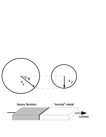
Figure 1: Top: Fermi surfaces of a heavy Fermi liquid (HFL) metal (left) and a “normal” light fermion metal (right). Bottom: an experimental setup where the HFL and “normal” metal coexist in the same sample and an electrical current flows through.

II Model Hamiltonian

We consider a Kondo lattice model for the metal, with a single band $\epsilon(\bm{k})$ of conduction ($\hat{c}_{\bm{k},\sigma}$) electrons with Bloch momentum $\bm{k}$ and spin $\sigma=\pm 1/2$, interacting antiferromagnetically with the localized $f$ electrons in a lattice with $N_{s}$ sites:

$$\hat{H} = \sum_{{\bm{k}},\sigma}\left(\epsilon(\bm{k})-\mu\right)\hat{c}_{{\bm{k}},\sigma}^{\dagger}\hat{c}_{{\bm{k}},\sigma}+\sum_{{\bm{k}},\sigma}\left(\epsilon_{f}-\mu\right)\hat{f}_{{\bm{k}},\sigma}^{\dagger}\hat{f}_{{\bm{k}},\sigma}$$ (1)

$$- J\sum_{i}\hat{\bm{s}}_{i}\cdot\hat{\bm{S}}_{i}\,,$$

with $J<0$, and the spin operators at site $i$ are given by $\hat{\bm{s}}_{i}=\hat{c}_{i,\alpha}^{\dagger}\bm{\sigma}\hat{c}_{i,\beta}$ and $\hat{\bm{S}}_{i}=\hat{f}_{i,\alpha}^{\dagger}\bm{\sigma}\hat{f}_{i,\beta}$ ($\bm{\sigma}$ are Pauli matrices). There is exactly one $f$ electron at each site. In order to describe the spin singlet formation between $c$ and $f$ electrons at every site in the HFL phase, we recast the local spin exchange interaction as $\hat{\bm{s}}_{i}\cdot\hat{\bm{S}}_{i}=-\left(\hat{\lambda}_{i,\uparrow}+\lambda_{i,\downarrow}\right)^{2}-\hat{n}_{c,i}-\hat{n}_{f,i}-\hat{n}_{c,i}\hat{n}_{f,i}$, where $\hat{n}_{c(f),i}$ is the number operator for $c$ ($f$) electron at site $i$ and $\hat{\lambda}_{i\sigma}=\frac{1}{2}\left(\hat{c}_{i,\sigma}^{\dagger}\hat{f}_{i,\sigma}+h.c.\right)$. We decouple the $\hat{\lambda}$ operators by introducing an auxiliary field, $\lambda$, so the effective mean field theory becomes newns :

$$\hat{H} = \sum_{{\bm{k}},\sigma}(\epsilon(\bm{k})-\mu)\hat{c}_{{\bm{k}},\sigma}^{\dagger}\hat{c}_{{\bm{k}},\sigma}+\sum_{{\bm{k}},\sigma}(\epsilon_{f}-\mu)\hat{f}_{{\bm{k}},\sigma}^{\dagger}\hat{f}_{{\bm{k}},\sigma}$$ (2)

$$- 2\lambda J\sum_{i,\sigma}\left(\hat{c}_{i,\sigma}^{\dagger}\hat{f}_{i,\sigma}+h.c.\right)-4\lambda^{2}JN_{s}\,.$$

In the HFL phase ($\lambda\neq 0$) quasi-particles form, with momentum $\bm{k}$, having $c$ and $f$ components. We shall assume that only the lowest band $E(\bm{k})$ of heavy quasi-particles is occupied. In the “normal” phase ($\lambda=0$) quasi-particles are just $c$ electrons. Single particles are described by two-component wave-functions $\psi(\bm{r})=(u(\bm{r}),v(\bm{r}))$ related to the $c$ and $f$ components of the electronic states, respectively, and obeying the normalization condition $|u(\bm{r})|^{2}+|v(\bm{r})|^{2}=1$. In homogeneous heavy fermion metals we have $(u(\bm{r}),v(\bm{r}))=(u_{\bm{k}},v_{\bm{k}})e^{i\bm{k}\cdot\bm{r}}$, with

$$u_{\bm{k}}^{2} = \frac{(2\lambda J)^{2}}{(2\lambda J)^{2}+\left(E-\epsilon(\bm{k})\right)^{2}}\,,$$ (3)

$$v_{\bm{k}}^{2} = \frac{\left(E-\epsilon(\bm{k})\right)^{2}}{(2\lambda J)^{2}+\left(E-\epsilon(\bm{k})\right)^{2}}\,,$$ (4)

and the energy of this state is

$$E(\bm{k})=\frac{1}{2}\left[\epsilon_{f}+\epsilon(\bm{k})\pm\sqrt{\left(\epsilon_{f}-\epsilon(\bm{k})\right)^{2}+(4\lambda J)^{2}}\right]\,.$$ (5)

In a normal homogeneous metal $u_{\bm{k}}=1$ for a $c$ electron and $v_{\bm{k}}=1$ for a local $f$ electron. The self-consistent equation for $\lambda$ is: $\lambda=(4N_{s})^{-1}\sum_{i,\sigma}\langle\hat{c}_{i,\sigma}^{\dagger}\hat{f}_{i,\sigma}+h.c.\rangle\,.$ In mean field theory, the local chemical potential $\epsilon_{f}$ for the $f$ electrons must be chosen so as to implement single occupancy on average, $\langle\hat{n}_{f,i}\rangle=1$, at every site $i$. Therefore, in a inhomogeneous system $\epsilon_{f}$ may be required to vary from site to site. In the HFL phase $\lambda\neq 0$ and both $c$ and $f$ electrons contribute to the FS volume. Therefore, the volume of the FS must either include $n_{c}$ electrons in the normal metal or $1+n_{c}$ electrons in the heavy fermion metal.

We now consider a system where both HFL and normal phases exist simultaneously and are separated by a thin interface. We take half of the metal ($x<0$) to be in the HFL phase while the other $x>0$ half is in the normal state ($\lambda=0$). The interface is the $yz$ plane. We shall denote by $\bm{p}$ the Bloch wave-vector in the heavy metal and by $\bm{k}$ the wave-vector in the normal metal.

III Interface properties

III.1 Absence of a proximity effect

If we consider that $J=0$ on the normal $x>0$ half of the metal, then the amplitude for singlet formation, $\langle\hat{c}_{i,\sigma}^{\dagger}f_{i,\sigma}\rangle$, drops abruptly from its finite value in the heavy fermion ($x<0$) metal, to zero in the normal metal next . The local singlet correlation $\lambda$ vanishes abruptly as one goes from the heavy to the normal metal because of the localized nature of the $f$ electrons. In this sense, we may say that there is no proximity effect for singlet formation. In a normal-superconductor interface there is a proximity effect for the pairing, $\langle c_{i,\uparrow}c_{i,\downarrow}\rangle$, because the electrons establish the Cooper pairing in the superconductor and they both propagate into the normal side transporting the correlation with them. This does not happen in the case discussed here since the $f$ electrons are localized. The coupling $J=0$ on the normal side effectively removes the normal metal $f$ local moments from the problem, so they cannot establish singlet correlations with conduction electrons. Nevertheless, there is a singlet correlation between a conduction electron on the normal side (close to the interface) and a $f$ moment on the heavy metal side. The same happens if, instead of taking $J=0$, a sufficiently strong magnetic field is applied to the $x>0$ portion of the metal which polarizes the $f$ moments, thereby preventing the formation of spin singlets. Alternatively, we may consider a temperature gradient, such that the left side of the sample is below the Kondo temperature, $T_{K}$, and the right hand side is above $T_{K}$. Then $\langle\hat{c}_{i,\sigma}^{\dagger}f_{i,\sigma}\rangle$ decreases continuously to zero as the temperature crosses $T_{K}$. The coherence factors of the quasi-particles $u$ and $v$ vary continuously in space but the FS volume of carriers changes abruptly in a very thin region where $\lambda\rightarrow 0$. The absence of a proximity effect is rather important in the case of inhomogeneous alloys because it shows that the heavy-fermion component of the system cannot penetrate the light component. The situation here is similar to the one in optics where light coming to an interface between two materials with very different index of refraction is completely reflected at the interface.

III.2 Formation of a dipole barrier

The spin singlet formation between localized $f$ and conduction electrons lowers the effective local site energy of the $c$ electron. This causes the chemical potential $\mu$ of a heavy fermion system to be lower than that of a normal metal with the same conduction electron concentration $n_{c}$. It implies that some conduction electrons initially flow through the interface, leaving a positive excess charge in the normal metal side and a negative excess charge on the heavy fermion side. Therefore, a dipole barrier forms close to the interface. The electrostatic potential created by the barrier (similar to that of a capacitor) increases the local site energy of the $c$ electrons on the heavy fermion subsystem by an amount $\epsilon_{c}$ with respect to the local $c$ site energies in the normal subsystem (the situation here resembles the contact potential of a dipole layer in p-n semiconductor junctions). The chemical potential is then constant throughout the sample but the $c$ site energies increase by the amount $\epsilon_{c}$ across the barrier from the normal to the heavy fermion side. Because these are metallic systems, the dipole barrier should be efficiently screened by the conduction electrons over a length of the order of few atomic spacings next .

Figure 2: Spatial variation of the $c$ site energies due to the formation of a dipole barrier at the interface.

The local site site energy of the $c$ electrons varies in space close to the interface, $\epsilon_{c}(x)=eV(x)$ where $V(x)$ is the electrostatic potential and $e$ is the electron charge. It is assumed that $V(x)\rightarrow 0$ as $x\rightarrow\infty$ deep inside the normal metal (see Figure 2). The Poisson equation for the local site energy reads

$$\frac{d^{2}\epsilon_{c}(x)}{dx^{2}}=-\frac{e^{2}}{\varepsilon_{0}}\left[n_{c}(x)-\bar{n}_{c}\right]\,,$$ (6)

where $\varepsilon_{0}$ is the vacuum electrical permitivity, $n_{c}(x)$ denotes the space dependent $c$ electron concentration and the value of $\bar{n}_{c}=n_{c}(\pm\infty)$ is determined by charge neutrality away from the interface. An analytical description of the dipole barrier can be made using a Thomas-Fermi approximation where the Fermi momenta are assumed to vary in space. On the heavy fermion side ($x<0$), using a parabolic dispersion, one can write:

$$\mu= \frac{1}{2}\left[\frac{\hbar^{2}p_{F}^{2}(x)}{2m}+\epsilon_{c}(x)+\epsilon_{f}\right.$$ (7)

$$\pm\left.\sqrt{\left(\frac{\hbar^{2}k_{F}^{2}(x)}{2m}+\epsilon_{c}(x)-\epsilon_{f}\right)^{2}+(4\lambda J)^{2}}\ \right]\,,$$

$$n_{c}(x) =\frac{2}{(2\pi)^{3}}\int_{0}^{p_{F}(x)}d^{3}p\ u_{p}^{2}(x)\,,$$ (8)

while on the normal metal side we write:

$$\mu = \frac{\hbar^{2}k_{F}^{2}(x)}{2m}+\epsilon_{c}(x)\,,$$ (9)

$$n_{c}(x) = \frac{2}{(2\pi)^{3}}\frac{4}{3}\pi k_{F}^{3}(x)\,.$$ (10)

Eliminating $k_{F}(x)$ from (9)- (10) and solving for $n_{c}(x)$, we can then insert the result in (6) obtaining:

$$\frac{d^{2}\epsilon_{c}(x)}{dx^{2}}=-\frac{e^{2}}{\varepsilon_{0}}\left[\left(\frac{2m}{\hbar^{2}}\right)^{\frac{2}{3}}\frac{\left(\mu-\epsilon_{c}(x)\right)^{\frac{3}{2}}}{3\pi^{2}}-\bar{n}_{c}\right]\,,$$ (11)

for $x>0$. But

$$\bar{n}_{c}=\left(\frac{2m}{\hbar^{2}}\right)^{\frac{3}{2}}\frac{\mu^{\frac{3}{2}}}{3\pi^{2}}\,,$$

therefore,

$$\frac{d^{2}\epsilon_{c}(x)}{dx^{2}} = -\frac{e^{2}}{\varepsilon_{0}}\frac{1}{3\pi^{2}}\left(\frac{2m}{\hbar^{2}}\right)^{2/3}\frac{\left[\left(\mu-\epsilon_{c}(x)\right)^{\frac{3}{2}}-\mu^{\frac{3}{2}}\right]}{3\pi^{2}}$$ (12)

$$\approx \frac{e^{2}}{\varepsilon_{0}}\left(\frac{2m}{\hbar^{2}}\right)^{\frac{2}{3}}\frac{\mu^{\frac{1}{2}}}{2\pi^{2}}\ \epsilon_{c}(x)$$

implying that $\epsilon_{c}(x)=\epsilon_{c}(0)e^{-x/\xi_{n}}$ with the screening length inside the normal metal given by:

$$\xi_{n}^{-2}=\frac{e^{2}mk_{F}}{\varepsilon_{0}\hbar^{2}\pi^{2}}\,.$$ (13)

Considering the heavy fermion side ($x<0$), we may directly write the variation in $c$-electron density already linearized in the energy shift of the site energies:

$$n_{c}(x)-\bar{n}_{c}=-N_{F(h)}\left[\epsilon_{c}(x)-\epsilon_{c}(-\infty)\ \right]\,,$$ (14)

where $N_{F(h)}$ denotes the Fermi level density of states of the heavy fermion system (which can be taken at $x=-\infty$) and is given by

$$N_{F(h)}=\frac{2}{(2\pi)^{3}}\int d^{3}p\ \delta\left(\mu-E(\bm{p})\right)=\frac{mp_{F}}{\pi^{2}\hbar^{2}u^{2}(p_{F})}\,.$$ (15)

Then the linearized version of the Poisson equation (6) becomes:

$$\frac{d^{2}\epsilon_{c}(x)}{dx^{2}}=\frac{e^{2}}{\varepsilon_{0}}\frac{mp_{F}}{\pi^{2}\hbar^{2}u^{2}(p_{F})}\left[\epsilon_{c}(x)-\epsilon_{c}(-\infty)\ \right]\,,$$ (16)

which gives

$$\epsilon_{c}(x)=\epsilon_{c}(-\infty)+\left[\epsilon_{c}(0)-\epsilon_{c}(-\infty)\ \right]e^{x/\xi_{h}}\,,$$ (17)

with the screening length on the heavy metal side given by

$$\xi_{h}^{-2}=\frac{e^{2}mp_{F}}{\varepsilon_{0}\hbar^{2}\pi^{2}u^{2}(p_{F})}\,.$$ (18)

The value of $p_{F}$ can be simply obtained from the condition of charge neutrality far from the interface,

$$\frac{2}{(2\pi)^{3}}\int^{p_{F}}d^{3}p\ =1+\bar{n}_{c}\,.$$ (19)

III.3 Transmission through the interface

The two-component wave-function $\psi(\bm{r})$ varies across the interface in such a way that it describes a heavy quasi-particle for $x<0$ and a $c$ or localized $f$ electron for $x>0$. The $f$ electrons are localized and therefore carry no charge current. It is only the $c$ electron that transports charge (across the interface). This can also be readily seen from the microscopic conservation of the probability, $\partial_{t}|\psi(\bm{r})|^{2}=-\nabla\cdot\bm{j}$, with $|\psi(\bm{r})|^{2}=|u(\bm{r})|^{2}+|v(\bm{r})|^{2}$. For a parabolic dispersion, $\epsilon(\nabla)\propto\nabla^{2}$, one obtains the current for a $\bm{k}$ state as $\bm{j}=i\left(u\nabla u^{*}-u^{*}\nabla u\right)/\hbar$, implying that only $u(\bm{r})$ carries the current.

The matching conditions to be imposed on the wave-function are the continuity of $u(\bm{r})$ and the current conservation, which is only related to $u(\bm{r})$. In a model with parabolic electronic dispersion, $\epsilon(\bm{k})\propto k^{2}$, this would imply the continuity of the gradient of $u(\bm{r})$. The function $v(\bm{r})$ itself obeys no matching condition: $v(\bm{r})=1$ (or $0$) for a $f$ (or $c$) electron on the normal $(\lambda=0)$ side and, in the HFL side, where $\lambda\neq 0$, $v(\bm{r})$ is determined by the diagonalization of the Hamiltonian (2) and the matching condition for $u(\bm{r})$.

In a model where $\lambda$ changes abruptly from a finite value to zero at the interface, the local chemical potential $\epsilon_{f}$ and the $c$ electron site energy $\epsilon_{c}$ vary in space in a small region close to the interface. In the following we neglect this spatial variation and assume that $\epsilon_{c}>0$ is constant for $x<0$ and $\epsilon_{c}=0$ for $x>0$, and that $\epsilon_{f}$ also changes abruptly from its constant bulk value in the heavy fermion $x<0$ to $\epsilon_{f}=\mu$ for $x>0$. In order to calculate the conductance through the interface, we consider a model parabolic dispersion for the $c$ electrons. The Bloch wave-vector has both parallel ($\bm{k}_{||}$) and perpendicular ($k_{x}$) components to the interface. Introducing the position vector $\bm{r}=(y,z)$, the matching conditions for the wave-function describing an incident quasi-particle from the left imply $\bm{p}_{||}=\bm{k}_{||}$:

$$\psi_{L}(x<0) = e^{i\cdot\bm{p}_{||}\cdot\bm{r}}\left[\left(\begin{array}[]{c}u\\ v\end{array}\right)e^{ip_{x}x}+r_{k,p}\left(\begin{array}[]{c}u\\ v\end{array}\right)e^{-ip_{x}x}\right]\,,$$ (24)

$$\psi_{L}(x>0) = t_{k,p}\left(\begin{array}[]{c}1\\ 0\end{array}\right)e^{ik_{x}x}e^{i\cdot\bm{p}_{||}\cdot\bm{r}}\,,$$ (27)

with the transmission and reflection amplitudes given by:

$$t_{k,p}=u\frac{2p_{x}}{p_{x}+k_{x}}\,,\qquad r_{k,p}=\frac{p_{x}-k_{x}}{p_{x}+k_{x}}\,,$$ (28)

respectively. The momenta satisfy the energy conservation condition $E\left(\bm{p}_{||},p_{x}\right)=\epsilon\left(\bm{k}_{||}=\bm{p}_{||},k_{x}\right)$. Because the heavy fermion metal has the larger FS only incident electrons from the left making an angle $\theta<\arcsin(k_{F}/p_{F})$ with the $x$ axis are transmitted (see Fig. 1). A wave-function describing an incident conduction electron from the right is given by:

$$\psi_{R}(x<0) = t_{-p,-k}e^{i\cdot\bm{k}_{||}\cdot\bm{r}}\left(\begin{array}[]{c}u\\ v\end{array}\right)e^{-ip_{x}x}\,,$$ (31)

$$\psi_{R}(x>0) = e^{i\cdot\bm{k}_{||}\cdot\bm{r}}\left[\left(\begin{array}[]{c}1\\ 0\end{array}\right)e^{-ik_{x}x}+r_{-p,-k}\left(\begin{array}[]{c}1\\ 0\end{array}\right)e^{ik_{x}x}\right]\,,$$ (36)

with the transmission and reflection amplitudes given by:

$$t_{-p,-k}=\frac{1}{u}\frac{2k_{x}}{p_{x}+k_{x}}\,,\qquad r_{-p,-k}=\frac{k_{x}-p_{x}}{p_{x}+k_{x}}\,,$$ (37)

respectively.

III.4 Conductance through the interface

The transmission and reflection amplitudes are determined by the mismatch of the Fermi momenta of the two subsystems. Applying a voltage $V$ across the interface, the charge current flowing from right to left is landauer :

$$I=2e^{2}V{\cal S}\int\frac{d^{3}k}{(2\pi)^{3}}\delta(\mu-\epsilon(\bm{k}))\ \frac{\partial E}{\hbar\partial p_{x}}\ |t_{-p,-k}|^{2}$$ (38)

where ${\cal S}$ denotes the area of the interface. It can be shown from (5) that the heavy particle velocity $\partial E(\bm{p})/\partial p_{x}=u^{2}\partial\epsilon(\bm{p})/\partial p_{x}$. Equation (38) can be written as:

$$I = 2e^{2}V{\cal S}\int_{0}^{\pi/2}d\theta\sin\theta\int_{0}^{2\pi}d\phi\int_{0}^{\infty}\frac{k^{2}\ dk}{(2\pi)^{3}}\times$$ (39)

$$\delta\left(\hbar v_{F}\left(k-k_{F}\right)\right)\ \frac{u^{2}\hbar p_{x}}{m}\left(\frac{2k_{x}}{u(k_{x}+p_{x})}\right)^{2}$$

The integration is performed in the half sphere $\theta<\pi/2$ of incident momenta from the normal metal. On the Fermi Surface we write $k_{x}=k_{F}\cos\theta$ and $p_{x}=p_{F}\cos\theta$. The momenta on both sides of the interface are related by $p_{F}^{2}=\bm{p}_{||}^{2}+p_{x}^{2}$ and $k_{F}^{2}=\bm{k}_{||}^{2}+k_{x}^{2}$ with $p_{||}=k_{||}=k_{F}\sin\theta$. Therefore, we can rewrite (39) as

$$I=\frac{4e^{2}V{\cal S}k_{F}^{3}}{\pi h}\int_{0}^{\pi/2}\frac{\sqrt{p_{F}^{2}-k_{F}^{2}\sin^{2}\theta}\ \cos^{2}\theta\sin\theta\ d\theta}{\left[\sqrt{p_{F}^{2}-k_{F}^{2}\sin^{2}\theta}+k_{F}\cos\theta\right]^{2}}\,.$$ (40)

The conductance of a clean heavy fermion metal is given by

$$G_{0h}={\cal S}\frac{e^{2}}{h}\frac{p_{F}^{2}}{2\pi}\,.$$ (41)

The conductance of the interface, $G_{i}(=I/V)$, obtained from equation (40) after changing the variable of integration to $x=\sin\theta$ is:

$$\frac{G_{i}}{G_{0h}}=8\kappa^{3}\int_{0}^{1}dx\frac{x\sqrt{1-x^{2}}\ \sqrt{1-\kappa^{2}x^{2}}}{\left[\sqrt{1-x^{2}}+\sqrt{1-\kappa^{2}x^{2}}\ \right]^{2}}\,,$$ (42)

where $\kappa^{3}=(k_{F}/p_{F})^{3}=n_{c}/(1+n_{c})$. Figure 3 shows a plot of the interface conductance versus $n_{c}$. One can clearly see that the larger the value of $n_{c}$ the larger is the effect and even for dense systems with $n_{c}=1$ electron per unit cell (half-filling) the value of the interface conductance is of the order of 60 % of that of a clean heavy fermion metal.

Figure 3: Interface conductance (normalized to that of a clean heavy fermion metal) plotted versus conduction electron density.

IV Experimental realization

In the geometry suggested in Fig. 1 with the heavy-fermion, the normal fermion, and the interface in series, one would measure the total conductance of the junction, that is, $G^{-1}=G_{h}^{-1}+G_{n}^{-1}+G_{i}^{-1}$, where $G_{n}$ is the conductance of the normal Fermi liquid. Hence, in order to measure the interface conductance one would have to measure the heavy and normal conductance separately, before measuring the conductance of the interface. The bulk conductance of the heavy fermion can be expressed as

$$G_{h}={\cal S}\frac{e^{2}}{h}\frac{p_{F}^{2}}{2\pi}\frac{\ell_{c}}{L}\,,$$ (43)

where $\ell_{c}$ is $4/3$ of the electron’s transport mean-free path and $L$ is the size of the system (in the clean limit, $\ell_{c}>L$, we set $L/\ell_{c}=1$ in (43)). Electron scattering by impurities and phonons are included in the bulk conductances. The point we wish to emphasize is that the interface itself causes a contribution to the total resistance.

The interface can be created avoiding large lattice mismatches between the two sides, so as to minimize structural scattering. Here we suggest a few possibilities: (1) in the scenario of Figure 4a, a large magnetic field can be applied to one side of the sample and the longitudinal resistivity can be measured with and without the field; (2) a sharp temperature gradient can be applied to a sample of a heavy fermion material so that half of the system is above the Kondo temperature and half is below the Kondo temperature. Heavy fermion materials have resistivity $\rho(T)\propto\log T$ above the Kondo temperature $T_{K}$ and $\rho(T)$ decreases rapidly as temperature is reduced below $T_{K}$. If a constant temperature difference is imposed across the sample with thermal conductivity $K$, a heat current $j_{Q}=K\ dT/dx$ flows. From the Wiedemann-Franz law we expect $dT/dx\propto T^{-1}\rho(T)$. If a material with a sharp resistivity peak near the Kondo temperature is chosen, then the temperature gradient is high in the region where $T\approx T_{K}$, producing a thin interface. In this case, the material must be chosen so as to minimize effects associated with thermoelectric power; (3) in the scenario of Figure 4b, for systems where the magnetic behavior can be tuned by changing the chemical concentration (chemical pressure), a sample could be grown with a large gradient concentration so that half of the system is in the magnetically ordered phase and half in the HFL phase; (4) alternatively, two different mechanical pressures can be applied on two regions of the sample, so that the two regions are on opposite sides of a QCP, as the points A and B in Figure 4b. If the QCP occurs at vanishing Kondo temperature, $T_{K}^{(1)}$, the sharp FS volume mismatch at the interface causes the effects predicted above.

Figure 4: a) The Kondo temperature decreases under external magnetic field and vanishes at a quantum critical point (QCP); b) phase diagram showing the QCP between an antiferromagnetic metal (AFM) and HFL phases, obtained by varying pressure.

In systems where the Kondo temperature is finite at the QCP ($T_{K}^{(2)}$ in Fig. 4(b)), we believe the interface scattering between the AFM and the HFL phases to be negligible small (and would anyway disappear as A and B approach the QCP). This can be seen as follows. The AFM, in this case, is a spin-density-wave (SDW) in a system where the local magnetic moments have been Kondo screened by the conduction electrons. Some regions of the Fermi surface are gapped. Now suppose that the electrons flow from the SDW to the paramagnetic phase. Only the electrons in the ungapped regions of the Fermi surface produce a current. An ungapped electron flows from the SDW into the paramagnetic phase without changing its Bloch $\bm{k}$ state. If an interface scattering exists at all, it should be very small, unlike the one predicted above for the Kondo screening scenario, which is caused by an appreciable momentum mismatch around the whole Fermi surface. Therefore, we believe that an experimental setup like the one we propose can distinguish the two scenarios ($T_{K}^{(1)}$ and $T_{K}^{(2)}$ in Fig. 4(b)) for the QCP in heavy fermion systems, because in the SDW scenario the interface scattering effect should be almost non-existent.

In summary, we have studied the problem of the transport through an interface between a heavy electron metal and an ordinary metal. We have argued that the heavy fermion state does not induce a proximity effect on the ordinary metal and that the hybridization gap changes abruptly across the interface. Because of the change of the $f$ electron energy across the interface an atomically thin dipole barrier is formed, a situation quite similar to the dipole layers in semiconducting p-n junctions. We have also shown that the interface produces a contribution to the electrical conductance that depends essentially on the number of electrons in the system and that for dense systems the value of the conductance is substantial and can be easily measured experimentally. We have also proposed ways to create such interfaces. We hope this work will stimulate experimentalists to realize them experimentally. Finally, we would like to stress that our results not only have implications for the problem of the nature of the heavy electron ground state, but also can be used to understand quantum criticality and the effects of inhomogeneities close to quantum critical points.

We thank L. Greene, G. Murthy, and G. Stewart for illuminating conversations. M.A.N.A. is grateful to Fundação para a Ciência e Tecnologia for a sabbatical grant. A. H. C. N. was supported by the NSF grant DMR-0343790.

References

- (1) S. Sachdev, Quantum Phase Transitions (Cambridge University Press, Cambridge, 1999).
- (2) A. Kopp, and S. Chakravarty, Nature Phys. 1, 53 (2005).
- (3) J. Custers, P. Gegenwart, H. Wilhelm, K. Neumaier, Y. Tokiwa, O. Trovarelli, C. Geibel, F. Steglich, C. Pepin, P. Coleman Nature 424, 524 (2003).
- (4) D. M. Newns, and N. Read, Adv. in Phys. 36, 799 (1987).
- (5) S. Pashen, T. Lühmann, S. Wirth, P. Gegenwart, O. Trovarelli, G. Geibel, F. Steglich, P. Coleman and Q. Si, Nature 432, 881 (2004)
- (6) A. H. Castro Neto, and B. A. Jones, Phys. Rev. B 62, 14975 (2000).
- (7) E. Miranda, and V. Dobrosavljevic, Rep. Prog. Phys. 68, 2337 (2005).
- (8) A. H. Castro Neto, and B. A. Jones, Europhys. Lett. 71, 790 (2005); Europhys. Lett., 72,1054 (2005).
- (9) A. J. Millis, D. Morr, and J. Schmalian, Europhys. Lett. 72, 1052 (2005).
- (10) W. K. Park, L. H. Greene, J. L. Sarrao, and J. D. Thompson, Phys. Rev. B 72, 052509 (2005); ibid., cond-mat/0507353.
- (11) G. R. Stewart, Rev. Mod. Phys. 73, 797 (2001).
- (12) M. A. N. Araújo, and A. H. Castro Neto, unpublished.
- (13) S. Datta, Electronic Transport in Mesoscopic Systems, (Cambridge, 1997).