Non-equilibrium Entanglement and Noise in Coupled Qubits

Abstract

We study charge entanglement in two Coulomb-coupled double quantum dots in thermal equilibrium and under stationary non-equilibrium transport conditions. In the transport regime, the entanglement exhibits a clear switching threshold and various limits due to suppression of tunneling by Quantum Zeno localisation or by an interaction induced energy gap. We also calculate quantum noise spectra and discuss the inter-dot current correlation as an indicator of the entanglement in transport experiments.

Precise engineering and preparation of entangled states forms the backbone of many quantum information schemes M. A. Nielsen, and I. L. Chuang (2000). The complete control of interactions between two or more parties is a sangraal that is not without cost. For example, in superconducting nano-circuits Y. Nakamura, Yu. A. Pashkin, and J. S. Tsai (1999) there has been much success in devising schemes for tunable capacitative couplings D.V. Averin and C. Bruder (2003), but thermal fluctuations, background noise and limited control over natural interactions must be dealt with and overcome in increasingly imaginative ways.

In this Letter, we take a slightly different point of view and ask for the degree of entanglement between two parallel, interacting electronic conductors under the ‘un-favourable’ condition of stationary currents passing through both of them. As this is clearly a mixed-state situation, we specifically consider a non-equilibrium version of the concurrence as entanglement measure for an electron charge double qubit (DQ), realised in Coulomb-coupled double quantum dots T. Hayashi, T. Fujisawa, H.-D. Cheong, Y.-H. Jeong, Y. Hirayama (2003); T. Brandes (2005) that are strongly coupled to external electron reservoirs at high voltage bias. We compare this to the same closed device in equilibrium with a heat bath, and our findings suggest that such an approach, although probably not directly relevant for quantum information purposes, sheds a new light on the relation between entanglement and the electronic transport process itself. In particular, effects like suppression of non-resonant tunneling and the quantum Zeno effect (QZE) have a direct impact on the entanglement, to which we also establish a further link by calculating the non-equilibrium quantum shot-noise tensor whose off-diagonal elements, as a function of the system parameters, show a behavior very similar to the concurrence.

Model.– For the sake of clarity, we define the double qubit by ‘left’ and ‘right’ orbital charge states $|\alpha_{i}\rangle$, $\alpha=L,R$ of one additional electron on top of the many-body ground state $|0_{i}\rangle$ (limit of intradot Coulomb interaction $U_{\rm in}\to\infty$) of two double quantum dots $i=1,2$ which are coupled by a single matrix element $U$ for inter-dot ’same site’ interactions (left-left and right-right), cf. Fig. (1). Tunnelling of electrons occurs only within but not between the qubits due to coupling $T_{i}$ in each double dot. Using projectors onto these orbital states, ($\hat{n}_{L}^{(i)}=|L\rangle\langle L|_{i}$, $\hat{n}_{LR}^{(i)}=|L\rangle\langle R|_{i}$,…), the total Hamiltonian is

$${\mathcal{H}}_{0} = \sum_{i=1,2}\left(\varepsilon_{i}(\hat{n}_{L}^{(i)}-\hat{n}_{R}^{(i)})+T_{i}(\hat{n}_{LR}^{(i)}+\hat{n}_{RL}^{(i)})\right)$$ (1)

$$+ \frac{U}{2}\left(\hat{n}_{L}^{(1)}\hat{n}_{L}^{(2)}+\hat{n}_{R}^{(1)}\hat{n}_{R}^{(2)}\right).$$

The electron spin label is suppressed here and in the following, as only charge states (acting as pseudo-spin) play a role. This description has turned out to be useful for modelling charge-related properties such as decoherence and noise in individual double quantum dots R. Aguado, T. Brandes (2004); T. Brandes (2005).

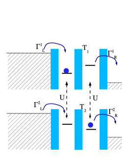
Figure 1: Transport double qubit model: left-right charge states in two Coulomb-coupled double quantum dots with one additional electron each and ‘on-site’ ($LL$, $RR$) interaction $U$, coherent tunnel couplings $T_{1}$ and $T_{2}$ and electron reservoir tunnel rates $\Gamma^{1/2}_{L/R}$.

We ‘open’ the DQ by coupling it to four external electron reservoirs, ${\mathcal{H}}={\mathcal{H}}_{0}+{\mathcal{H}}_{T}+{\mathcal{H}}_{\rm res}$, with ${\cal H}_{\rm res}=\sum_{i=1,2}\sum_{\alpha\in L,R}\sum_{ki\alpha}\epsilon_{ki\alpha}c_{ki\alpha}^{\dagger}c_{ki{\alpha}}^{\phantom{\dagger}}$ ($\alpha=L/R$ refers to left and right reservoirs for qubit number $i$, $i=1,2$) and ${\cal H}_{T}=\sum_{i=1,2}\sum_{\alpha\in L,R}\sum_{k}(V_{k}^{\alpha i}c_{ki{\alpha}}^{\dagger}\hat{s}_{\alpha}^{i}+H.c.)$, with Hubbard operators $\hat{s}_{\alpha}^{i}=|0_{i}\rangle\langle\alpha_{i}|$ that couple the qubits to the continuum.

Equilibrium entanglement.– If the DQ is disconnected from the reservoirs (${\mathcal{H}}_{T}=0$) but in contact with a heat bath at temperature $T=1/\beta$, the equilibrium entanglement between qubit 1 and 2 is easily obtained from the concurrence W. K. Wootters (1998) (a well-known entanglement measure of mixed states of two qubits) $C(\beta)$ for the canonical ensemble state $\rho(\beta)=e^{-\beta{\mathcal{H}}_{0}}/Z$, $Z={\rm Tr}e^{-\beta{\mathcal{H}}_{0}}$. The eigenvectors of ${\mathcal{H}}_{0}$ correspond to eigenvalues $E_{0}=0$, $E_{1}=U$, and $E_{\pm}=(U\pm\sqrt{16T_{c}^{2}+U^{2}})/2$ and are expressed in the basis of singlet and triplet states, $S_{0}=1/\sqrt{2}(|L_{1}R_{2}\rangle-|R_{1}L_{2}\rangle)$, $T_{+}=|L_{1}L_{2}\rangle$, $T_{-}=|R_{1}R_{2}\rangle$, $T_{0}=1/\sqrt{2}(|L_{1}R_{2}\rangle+|R_{1}L_{2}\rangle)$. For simplicity we restrict ourselves to the unbiased, symmetric case $\varepsilon_{i}=0$, $T_{i}=T_{c}(i=1,2)$. It turns out that the equilibrium case already exhibits some interesting features, cf. Fig.(2). At any finite temperature $T$, the entanglement is zero below a certain threshold value of the interaction $U$ where the state $\rho(\beta)$ is too mixed in order to be entangled which is, e.g., in analogy with the corresponding transition in the (abstract) example of the Werner state R. F. Werner (1989). Furthermore, the concurrence shows a non-monotonic behaviour as a function of $U$ at fixed $T$, with an entanglement maximum at an optimal $U$-value.

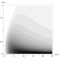
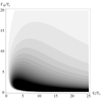
Figure 2: Left: Grey-scale plot of double qubit equilibrium concurrence as a function of interaction $U/T_{c}$ and temperature $T/T_{c}$ (white is zero, black is maximum $C=1$ ). In all of the following results both devices have identical parameters $\Gamma_{L}^{(i)}\equiv\Gamma_{L}$, $\Gamma_{R}^{(i)}\equiv\Gamma_{R}$, $T_{i}\equiv T_{c}$, for $i=1,2$. Right: Concurrence of non-equilibrium double qubit as a function of interaction $U/T_{c}$ and reservoir tunnel rate $\Gamma_{R}$ for large $\Gamma_{L}/T_{c}=50$. Zero entanglement occurs below a threshold $\propto 1/\Gamma_{R}$ in the weak tunnelling regime, and for very strong tunnelling $\Gamma_{R}\gg T_{c}$ due to Zeno-localisation, cf. text. (Black is the maximum $C=0.3$).

Stationary transport.– The limit $t\to\infty$ in the dynamical evolution of the reduced DQ density operator $\rho$ defines a stationary non-equilibrium state $\rho_{\infty}$ which usually is much more difficult to determine than in the equilibrium case. Transport properties of models like Eq.(1) can be analysed by using various non-equilibrium techniques. Here, we consider a specific limit of infinite source-drain bias in order to obtain quasi-analytic results from a generalised Master equation, $\dot{\rho}={L}[\rho]$. The super-operator $L$ is parametrized by the Markovian DQ-lead tunnel rates $\Gamma_{\alpha}^{i}\equiv 2\pi\sum_{k}|V_{k}^{\alpha i}|\delta(\varepsilon-\epsilon_{ki{\alpha}})$ (of which the energy-dependence is neglected), and the DQ parameters $\varepsilon_{i}=0$, $T_{i}=T_{c}(i=1,2)$. Analytical expressions for the stationary solution of the 25 coupled equations of motion (EOM) can then be found in an approximation where the broadening due to tunnelling of the DQ levels is neglected, which for $\varepsilon_{i}=0$, however, is only a very crude approximation.

One obtains better results for the stationary currents $\langle I_{i}\rangle_{\infty}$ by second order perturbation theory in the intra-dot tunnel couplings $T_{i}$, which clearly show a tunnel-broadened resonance

$$\langle I_{i}\rangle_{\infty}=-e\frac{\Gamma_{R}^{i}T_{i}^{2}}{(\Gamma_{R}^{i}/2)^{2}+U^{2}}$$ (2)

($-e$ is the electron charge). In this limit, the resonance is determined by the energy gap $U$ between the localised eigenstates of the DQ: at large $U$, the triplet $T_{+}=|L_{1}L_{2}\rangle$ becomes populated (note that this state is always available because of the infinite voltage approximation). The energy gap to any other state involving delocalized electrons (e.g, the triplet $T_{0}$ or the singlet $S_{0}$) then suppresses the elastic current. In analogy to single charge qubits, where the energy gap is given by the internal bias $\varepsilon$, we expect this suppression to be lifted in the presence of inelastic processes Fujetal98 .

Furthermore, as a function of the coupling $\Gamma_{R}^{i}$ to the drain, the current first increases and then becomes smaller again. With the drains acting as broadband measuring devices (electron on right side or not), strong couplings $\Gamma_{R}^{i}\to\infty$ completely freeze the charges on the left sides which is a ‘transport version’ example Y. N. Chen, T. Brandes, C. M. Li, and D. S. Chuu (2004) of the QZE.Alternatively, this localisation can be interpreted as an infinite level broadening and the corresponding suppression of the local spectral density due to the decay to the drain. Finally, the behaviour of the current, cf. Eq.(2), follows the occupation of the entangled singlet state $S_{0}$ as illustrated in the inset of Fig.(3). The main current contribution therefore stems from two-particle tunneling events, which in turn motivates our later comparison of the concurrence with the current fluctuations.

Non-equilibrium entanglement.– We now define the non-equilibrium entanglement via the concurrence $C$ of the stationary state $\hat{P}\rho_{\infty}$, where $\hat{P}$ is the projection onto doubly occupied states including proper normalisation; i.e. we calculate the concurrence when both double dots have a single electron in them and there are thus two two-state systems to be entangled. The projection $\hat{P}$ corresponds to taking the limit $\Gamma_{L}^{i}\to\infty$ where both qubits are always occupied with one single electron. For example, for $U=0$ and $\Gamma_{L}\to\infty$, the stationary state of a single charge qubit is described by the (Bloch) vector of pseudo-spin Pauli matrices ($\varepsilon\equiv\varepsilon_{L}-\varepsilon_{R}$)

$$\langle\vec{\sigma}\rangle=\left(\frac{2T_{c}\varepsilon}{\mathcal{N}},\frac{\Gamma_{R}T_{c}}{\mathcal{N}},\frac{\Gamma_{R}^{2}/4+\varepsilon^{2}}{\mathcal{N}}\right),$$ (3)

with $\mathcal{N}\equiv\Gamma_{R}^{2}/4+\varepsilon^{2}+2T_{c}^{2}$ and in the $L$-$R$ basis where $\sigma_{z}\equiv|L\rangle\langle L|-|R\rangle\langle R|$ etc. For $U\neq 0$, we numerically checked that $\hat{P}\rho_{\infty}=\lim_{\Gamma_{L}^{i}\to\infty}\rho_{\infty}$ which means that the two-qubit concurrence $C$ defined in this way does no longer depend on the left tunnel rates. This is a good description of non-equilibrium entanglement in a real system as long as $\Gamma_{L}^{i}\gg$max$(U,\Gamma_{R}^{i},T_{c},\varepsilon)$.

As $C$ is zero to second order in $T_{c}$, we use numerical results, cf. Fig.(2), which shows an intriguing behaviour of the concurrence as a function of $U$ and the tunnel rate $\Gamma_{R}^{i}\equiv\Gamma_{R}$. We find a switching threshold in that below an interaction strength $U\sim 2T_{c}^{2}/\Gamma_{R}$ the entanglement is zero: for small $\Gamma_{R}$, the stationary currents become very small, cf. Eq. (2), and thus strong interactions are required in order to entangle the dots. The DQ state becomes strongly mixed for $\Gamma_{R}\to 0$ (note that we have not taken into account any additional, internal relaxation processes here); its zero entanglement along the axis $\Gamma_{R}=0$ is in fact a continuation of the point $U=0$ where the states of both qubits are located at the origins of their Bloch spheres, cf. Eq. (3).

On the other hand, for very large $\Gamma_{R}$ one runs again into the QZE with electrons becoming trapped on the left ($\langle\sigma_{z}\rangle\to 1$, cf. Eq. (3)), and $\hat{P}\rho_{\infty}$ approaching the (pure) localised state $|L_{1}L_{2}\rangle$ which has zero entanglement. Finally, an increase from small to larger $\Gamma_{R}$ at fixed $U$ yields the re-entrance behaviour visible in the ‘teardrop’-shaped region of large entanglement in Fig. (2).

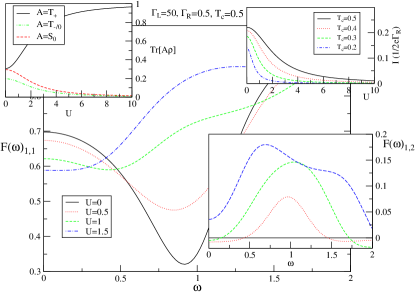
Figure 3: Main: Diagonal noise spectrum $F(\omega)_{1,1}=S(\omega)_{1,1}/2eI$. The resonance at $\omega=2T_{c}$ splits into new resonance points at the Bohr Frequencies $\lambda_{\pm}=E_{1}-E_{\pm}=1/2(U\mp\sqrt{16T_{c}^{2}+U^{2}})$. Top right inset: Stationary current $I_{\text{stat}}$. Top left inset: Occupation of several singlet and triplet states. Bottom Inset: The cross-correlation frequency spectrum $F(\omega)_{1,2}=S(\omega)_{1,2}/2eI$. Again resonance points manifest, however the correlation is always zero for $U=0$ and can assume negative values for $U\neq 0$.

Non-equilibrium noise: formalism.– Turning now to our description of non-equilibrium shot-noise and its relation to entanglement, the stationary state $\rho_{\infty}$ on its own is not sufficient in order to describe intrinsic properties of the DQ: for example, only limited information on the spectrum can be obtained from stationary quantities like the current. In contrast, the shot-noise spectrum exhibits resonances at the transition frequencies of the system and contains furthermore useful information on its relaxation and dephasing properties R. Deblock, E. Onac, L. Gurevich and L. P. Kouwenhoven (2003); D. A. Bagrets and Y. V. Nazarov (2003); G. Kießlich, A. Wacker, and E. Schöll (2003); R. Aguado, T. Brandes (2004). We will now also show an emergent resemblance in the behaviour of the current cross noise and the non-equilibrium concurrence as a function of the system parameters.

In general, the finite-frequency noise has contributions from particle currents as well as contributions from displacement currents Y. M. Blanter and M. Büttiker (2000); R. Aguado, T. Brandes (2004). In our case ($\Gamma_{L}^{i}\gg\Gamma_{R}^{i}$), however, it is a good approximation to consider only particle currents. Our starting point is the generating function

$$\hat{G}(s_{1},...,s_{m},t)=\sum_{n_{1},...n_{m}=0}^{\infty}s_{1}^{n_{1}}\cdot\cdot\cdot s_{m}^{n_{m}}{\rho}^{(n_{1}),...,(n_{m})}(t)$$ (4)

which, for an arbitrary number of $m$ qubits, contains the complete information on the tunnelling process as a function of time via the counting variables $s\equiv\{s_{i}\}$ and the conditional density matrices ${\rho}^{(n_{1}),(n_{2}),...}(t)$ for $n_{i}$ tunnelling events (‘jumps’) to the drain $i$ after time $t$. In matrix form, the EOM of the generating function follows from the Liouville equation for the conditional density matrices and reads $\dot{\textbf{G}}(s,t)=M(s)\textbf{G}(s,t)$ with formal solution $\textbf{G}(s,t)=\exp[tM(s)]\textbf{G}(s,0)$. General expectation values can be extracted from derivatives of $\text{Tr}[\textbf{G}(s,\tau)]$ with respect to the counting variables. In particular, the symmetrized noise correlation function $S(\omega)_{i,j}\equiv\int_{-\infty}^{\infty}e^{i\omega\tau}\langle\left\{\delta{I_{i}(t+\tau)},\delta{I_{j}(t)}\right\}\rangle$ between qubit $i$ and $j$ can then be written as a MacDonald formula D. K. C. MacDonald (1948); B. Elattari and S. A. Gurvitz (2002)

$$\frac{S(\omega)_{i,j}}{2e^{2}\omega} = \int_{0}^{\infty}d\tau\sin(\omega\tau)\frac{\partial}{\partial\tau}\left\langle n_{i}n_{j}-\frac{\tau^{2}\bar{I}_{i}\bar{I}_{j}}{e^{2}}\right\rangle$$ (5)

where $\langle n_{i}n_{j}\rangle=\hat{D}_{ij}\text{Tr}[\textbf{G}(s,\tau)]|_{s=1}$ with the differential operator $\hat{D}_{ij}\equiv\partial_{s_{i},s_{j}}+\delta_{ij}\partial_{s_{i}}$. We simplify this expression following Flindt et al. C. Flindt, T. Novotný, and A.-P. Jauho, Europhys. Lett.69, 475 ; Physica E 29, 411(2005) (2005) by introducing jump operators $L_{i}$ for qubit sources $i$ and writing $\partial_{\tau}\langle n_{i}n_{j}\rangle=\text{Tr}[L_{i}\sum_{n_{1},...,n_{m}}n_{j}\rho^{(n_{1}),...,(n_{m})}(\tau)]+(i\leftrightarrow j)$. This can be further evaluated by Laplace transforming the EOM $\partial_{t}\hat{G}(s,t)=(L_{0}+\sum_{i}s_{i}L_{i})\hat{G}(s,t)$ and taking derivatives in counting variables, giving $\partial_{s_{i}}\tilde{G}(s,-i\omega)|_{s=1}=F_{\omega}L_{i}F_{\omega}\rho_{0}$, where $F_{\omega}=(-i\omega-L)^{-1}$ and $\rho_{0}$ is the steady state initial condition. Using the projections $F_{\omega}=-P/i\omega-R_{\omega}$, $R_{\omega}=Q(i\omega+L)^{-1}Q$, ($P=\rho_{0}\otimes 1$, $Q=1-P$) with $P\rho_{0}=\rho_{0}$ and $Q\rho_{0}=0$ leads to

$$\frac{S(\omega)_{i,j}}{-2e^{2}} = \text{Re}\text{Tr}\left[\left(L_{i}R_{\omega}+\frac{\delta_{ij}}{2}\right)L_{j}\rho_{0}\right]+(i\leftrightarrow j).$$ (6)

In the zero frequency limit, we verify that the noise is determined as usual D. A. Bagrets and Y. V. Nazarov (2003); W. Belzig (2005) by the lowest eigenvalue $\lambda_{0}(s)$ of the matrix $M(s)$, namely by the long-time behaviour $G(s,t\to\infty)\propto\exp[t\lambda_{0}(s)]$ and therefore $S(0)_{i,j}={2e^{2}}\hat{D}_{ij}\lambda_{0}(s=1)$.

Non-equilibrium noise: results.– The currents through our two parallel charge qubits give rise to two diagonal and one off-diagonal component in the tensor $S(\omega)_{i,j}$ of the noise spectrum. In Fig.(3), we present results for the diagonal noise, i.e. the noise spectrum $S(\omega)_{1,1}=S(\omega)_{2,2}$ of the individual, interacting qubits. This spectrum clearly displays resonances at the Bohr frequencies as given by the excitation energies of the closed system. At $U=0$, there is one single resonance at $\omega=2T_{c}$ that splits up when $U$ is increased. Similar to light emission spectra in real molecules, frequency-dependent shot-noise spectra thus provide direct information about the correlated energy levels in artificial molecules.

The cross-noise spectrum exhibits a somewhat more complicated resonance structure (inset of Fig.(3)). More interesting is however the behaviour of the cross-correlation Fano factor at zero frequency, $F(0)_{1,2}\equiv S(0)_{1,2}/2eI$, which becomes positive as $U$ increases. This positive cross-correlation is an indication of correlated emission of electron pairs into different exit right leads positive . As a function of $U$, cf. in Fig.(4), there is a strong analogy between the cross-noise $F(0)_{1,2}$, its first derivative $F^{\prime}(0)_{1,2}$, and the non-equilibrium concurrence $C$, at least on a qualitative level. In particular, the non-analytic switching of $C$ with increasing $U$ from un-entangled to entangled states translates into a strongly delayed (though smooth) onset of the increase in $F(0)_{1,2}$, and the transition of $F^{\prime}(0)_{1,2}$ from negative to positive. For example, in the figure we see $F^{\prime}(0)_{1,2}$ for $T_{c}=0.5$ becomes positive around $U=1$ in agreement with the switching of $C$ at $U\sim 2T_{c}^{2}/\Gamma_{R}=1$. This analogy between noise and entanglement so far holds on a qualitative level only.

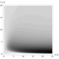
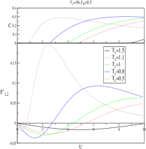
Figure 4: Left: The cross-correlation zero-frequency spectrum Fano Factor $F(0)_{1,2}=S(0)_{1,2}/2eI$. The resemblence to the concurrence, Fig. (2), is qualitative. (White is minimum, $F_{1,2}=-0.12$, black is maximum, $F_{1,2}=0.84$). Right: The switching phenomenon in the concurrence is more clearly seen, as well as a negative to positive re-emergence in the first derivative of the noise around the same point.

Finally, we mention that we have not included the effect of dissipation in our calculations so far. Weak decoherence processes can in principle be easily incorporated through additional terms within the master equation. In R. Aguado, T. Brandes (2004) it was shown how to use the resulting changes in the noise spectrum in order to extract, e.g., relaxation and decoherence times $T_{1}$ and $T_{2}$. This can also be done for the interacting qubits discussed here.

Conclusions We have shown how the entanglement of a non-equilibrium double qubit differs from its thermal-equilibrium relative by exhibiting a $1/\Gamma$ switching threshold for weak tunnelling rates $\Gamma$. The cross-correlation noise reflects this threshold at $\omega=0$ and shows resonances at the Bohr frequencies of the double qubit for finite $\omega$. Future theoretical work may include clarifying this relationship and checking the influence of decoherence on the correlated noise power spectrum.

Acknowledgements We would like to acknowledge discussions and suggestions from T. Novotný and S. Debald. Work supported by the Spanish MEC through grant MAT2005-07369-C03-03 and by the Japan Society for the Promotion of Science Grant 17-05761.

References

- M. A. Nielsen, and I. L. Chuang (2000) M. A. Nielsen, and I. L. Chuang, Quantum Computation and Quantum Information (Cambridge University Press, Cambridge, 2000).
- Y. Nakamura, Yu. A. Pashkin, and J. S. Tsai (1999) Y. Nakamura, Yu. A. Pashkin, and J. S. Tsai, Nature 398, 786 (1999).
- D.V. Averin and C. Bruder (2003) D. V. Averin and C. Bruder, Phys. Rev. Lett. 91, 057003 (2003).
- D. Loss, D. P. DiVincenzo (1998) D. Loss, D. P. DiVincenzo, Phys. Rev. A 57, 120 (1998).
- T. Hayashi, T. Fujisawa, H.-D. Cheong, Y.-H. Jeong, Y. Hirayama (2003) T. Hayashi, T. Fujisawa, H.-D. Cheong, Y.-H. Jeong, Y. Hirayama, Phys. Rev. Lett. 91, 226804 (2003).
- T. Brandes (2005) T. Brandes, Phys. Rep. 408(5), 315 (2005).
- R. Aguado, T. Brandes (2004) R. Aguado, T. Brandes, Phys. Rev. Lett. 92, 206601 (2004).
- W. K. Wootters (1998) W. K. Wootters, Phys. Rev. Lett. 80, 2245 (1998).
- R. F. Werner (1989) R. F. Werner, Phys. Rev. A 40, 4277 (1989).
- (10) T. Fujisawa, T. H. Oosterkamp, W. G. van der Wiel, B. W. Broer, R. Aguado, S. Tarucha, and L. P. Kouwenhoven, Science, 282, 932, (1998).
- Y. N. Chen, T. Brandes, C. M. Li, and D. S. Chuu (2004) Y. N. Chen, T. Brandes, C. M. Li, and D. S. Chuu, Phys. Rev. B 69, 245323 (2004).
- R. Deblock, E. Onac, L. Gurevich and L. P. Kouwenhoven (2003) R. Deblock, E. Onac, L. Gurevich and L. P. Kouwenhoven, Science 301, 203 (2003).
- D. A. Bagrets and Y. V. Nazarov (2003) D. A. Bagrets and Y. V. Nazarov, Phys. Rev. B 67, 085316 (2003).
- G. Kießlich, A. Wacker, and E. Schöll (2003) G. Kießlich, A. Wacker, and E. Schöll, Phys. Rev. B 68, 125320 (2003).
- D. K. C. MacDonald (1948) D. K. C. MacDonald, Rep. Progr. Phys. 12, 56 (1948).
- B. Elattari and S. A. Gurvitz (2002) B. Elattari and S. A. Gurvitz, Phys. Lett. A 292, 289 (2002).
- C. Flindt, T. Novotný, and A.-P. Jauho, Europhys. Lett.69, 475 ; Physica E 29, 411(2005) (2005) C. Flindt, T. Novotný, and A.-P. Jauho, Europhys. Lett. 69, 475 (2005); Physica E 29, 411 (2005).
- W. Belzig (2005) W. Belzig, Phys. Rev. B 71, 161301(R) (2005).
- Y. M. Blanter and M. Büttiker (2000) Y. M. Blanter and M. Büttiker, Phys. Rep. 336, 1 (2000).
- (20) See, for example, M. B uttiker, ”Reversing the sign of current-current correlations” in Quantum Noise, edited by Yu. V. Nazarov and Ya. M. Blanter, Kluwer, p. 3 - 31 (2003).