Surfaces of Constant Temperature for Glauber Dynamics

Abstract

The wavefunction of a single spin system in a prepared initial state evolves to equilibrium with a heat bath. The average spin

$$q(t)=p_{\uparrow}(t)-p_{\downarrow}(t)$$

exhibits a characteristic time for this evolution.

With the proper choice of spin flip rates, a dynamical Ising model (Glauber) can be constructed with the same characteristic time for transition of the average spin to equilibrium. The Glauber dynamics are expressed as a Markoff process that possesses many of the same physical characteristics as its quantum mechanical counterpart.

In addition, since the classical trajectories are those of an ergodic process (the time averages of a single trajectory are equivalent to the ensemble averages), the surfaces of constant temperature, in terms of the model parameters, may be derived for the single spin system.

I Background on the Example

The goal of this short note is to establish the surfaces of constant temperature consistent with the Glauber dynamics of a simple example. The example itself is taken from Glauber’s original paper glauber .

The subsystem of interest is a single spin particle in equilibrium with a heat bath. The total system consists of particle plus bath. The physical parameters are applied external field strength $H$ and temperature $\theta$. The particle is in a prepared initial state and evolves to a mixed state in equilibrium with the bath. The time constant for this evolution may be measured and used to construct a Markoff process with classical trajectories and the same decay time.

The inverse of the decay time is used as a rate (spin flips per unit time) parameter in the construction of the Markoff process and is denoted by $\alpha.$ The value of the average spin of the system at equilibrium is denoted by $\beta$ and is used to model the presence of a magnetic field. This situation is depicted in figure 1.

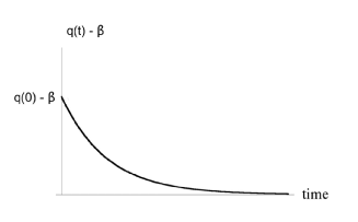
Figure 1: Relaxation of known average spin to its equilibrium value $\beta$ occurs exponentially with parameter $\alpha.$

At equilibrium the probability amplitudes correspond to Gibb’s distribution with Ising Hamiltonian $(\mu H,-\mu H)$ for the up and down states respectively. Note that for all values of H the sum of the subsystem energies is zero ford . By choosing the state transition rates of the classical trajectories appropriately, this too may be built into the Markoff process. See figure 2.

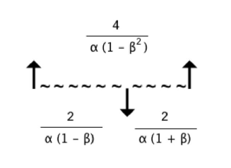
Figure 2: Characteristic holding times and total Carlson depth for the states of the single spin system

II Temperature Development

A large ensemble of N identical single spin subsystems are prepared. Once equilibrium with the bath has been attained, measurement reveals $N_{\uparrow}$ up and $N_{\downarrow}$ down. The ratio of the state probabilities is given simply by

$$\frac{p_{\uparrow}}{p_{\downarrow}}=\frac{N_{\uparrow}}{N_{\downarrow}}.$$

If the time evolution of a Markoff process is ergodic, the state probabilities may also be expressed in terms of the epochs of the average cycle behavior. See figure 2. Per characteristic cycle time, the associated equilibrium Markoff process (as defined by the state transition rates for the spins) spends

$$\Delta t_{\uparrow}=\frac{2}{\alpha(1-\beta)}$$

$$\Delta t_{\downarrow}=\frac{2}{\alpha(1+\beta)}$$

in the up and down states respectively. The probability ratios are given by

$$\frac{p_{\uparrow}}{p_{\downarrow}}=\frac{\frac{2}{\alpha(1-\beta)}}{\frac{2}{\alpha(1+\beta)}}=\frac{1+\beta}{1-\beta}.$$

At zero field, neither state $\uparrow$ or $\downarrow$ is preferred. The classical single particle system switches from one state to the other at random. In the language of the Glauber parameters this situation corresponds to

$$\alpha\neq 0,\,\beta=0.$$

Alternatively, in terms of the system temperature and applied field

$$\theta\neq 0,\,H=0.$$

Clearly, since the two languages describe the same phenomenon, there is an implied mapping between the $\theta-$axis in $(H,\theta)-$space and the $\alpha-$axis in the $(\alpha,\beta)-$space. In systems whose parameterization lies purely along either the $\alpha$ or $\theta-$axes, the amount of time spent spin up per characteristic period is equal to the amount of time spent spin down. This implies another pair of mappings between these axes and the line

$$\Delta t_{\uparrow}=\Delta t_{\downarrow}$$

in the time domain.

Note that for arbitrary constants $\lambda_{1}$ and $\lambda_{2}$, the transitions (dilatations)

$$(\Delta t_{\uparrow},\Delta t_{\downarrow})\longrightarrow(\lambda_{1}\,\Delta t_{\uparrow},\lambda_{1}\,\Delta t_{\downarrow})$$

and

$$(H,\theta)\longrightarrow(\lambda_{2}\,H,\lambda_{2}\,\theta)$$

leave the probabilities invariant. The direction of maximum probability gradient lies perpendicular to these invariant directions in either space. See figure 3.

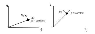
Figure 3: Observers agree on lines (constant probabilities) and circular arcs (maximum $\nabla p$) in both spaces.

In ford , these simple observations are used to construct the surfaces of constant temperature in time. That is, the image of the lines $\theta=$ constant, in the $(H,\theta)-$space, mapped to $(\Delta t_{\uparrow},\Delta t_{\downarrow})-$space via the relation

$$\theta(\Delta\mathbf{t})=\frac{\textrm{const.}}{\|\Delta\mathbf{t}\|_{2}\,\sqrt{(\log[\frac{\Delta t_{\uparrow}}{\Delta t_{\downarrow}}])^{2}+1}}.$$

These surfaces are presented in the left hand panel of figure 4. The right hand panel of the figure shows the same surfaces as seen from $(\alpha,\beta)$-space.

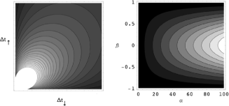
Figure 4: Lines of constant temperature as seen from the time domain coordinates ($\Delta t_{\uparrow}$, $\Delta t_{\downarrow}$) and in terms of the Markoff parameters ($\alpha$, $\beta$).

The implication is that, at constant temperature, the decay parameter $\alpha$ for the average spin $q(t)-\beta$ increases with increasing applied field parameter $\beta$.

III Bibliography

References

- (1) R. Glauber, “ Time Dependent Statistics of the Ising Model”, J. Math. Physics 4, 2, pp. 294-307, 1963
- (2) D. Ford, “Surfaces of Constant Temperature in Time,” http://www.arxiv.org/abs/cond-mat/0510291, 2005