Microwave response and spin waves in superconducting ferromagnets

Abstract

Excitation of spin waves is considered in a superconducting ferromagnetic slab with the equilibrium magnetization both perpendicular and parallel to the surface. The surface impedance is calculated, and its behavior near propagation thresholds is analyzed. The influence of nonzero magnetic induction at the surface is considered in various cases. The results provide a basis for the investigation of materials with coexisting superconductivity and magnetism by microwave response measurements.

I Introduction

The problem of the coexistence of superconductivity and magnetism has attracted renewed interest during the last decade due to the discovery of unconventional and high-$T_{c}$ superconductors, in which such a coexistence seems to be realized. The presence of magnetic properties has been supported by experimental evidence in such materials as high-$T_{c}$ ruthenocuprates, felner Sr₂RuO₄, luke ZrZn₂, Pfleiderer and UGe₂. Saxena

Experimental investigation of ferromagnetism coexisting with superconductivity is hampered by the fact that the spontaneous magnetic moment is screened by the Meissner currents in macroscopic samples. Therefore the usual methods, such as the Knight shift or muon spin relaxation, are only able to detect small remanent fields near inhomogeneities, defects etc. On the other hand, dynamical measurements - e. g.,  excitation of spin waves - provide a direct probe of bulk magnetization and are sensitive not only to its magnitude, but also the direction and degree of uniformity. There have been reports in the literature tallon of microwave measurements in powder or ceramic polycrystalline samples made of materials with coexisting superconductivity and magnetism (SCFM).

Theoretical research on macroscopic electromagnetic properties of SCFM’s was initiated by Ng and Varma, Ng ; Ng2 who have considered the bulk magnetic response and calculated the spin-wave modes for the spontaneous vortex phase. This regime, in which vortices are created in the sample without any applied magnetic field, is realized when the spontaneous magnetization is strong enough - namely, larger than $H_{c1}/4\pi$, with $H_{c1}$ being the first critical field. However, in order to make direct comparison with microwave experiments, the finite-sample response - namely, the surface impedance - is needed. Unlike in usual metals, dielectrics, or paramagnetics, this quantity cannot be trivially related to the bulk properties in SCFM’s, but requires a separate study. Hence the next step was done by the present author and Sonin, BS ; SW ; pwave who have considered the electromagnetic response of a thick slab, concentrating on the Meissner regime, in which static magnetic fields are screened in the bulk. In this regime, static magnetic measurements are difficult, and hence microwave experiments may be of particular interest. Spin-wave excitation and propagation were considered for a SCFM slab with the magnetization perpendicular to the surface (perpendicular geometry). BS While the analysis was initially carried for the case of Landau-Lifshitz (LL) SCFM’s with spin magnetism, the results have been generalized to the case of $p$-wave superconductors with orbital magnetism. pwave It was shown that these materials are in general described by more complicated magnetic dynamics than LL dynamics. However, two specific cases - namely, when the waves propagate either parallel or perpendicular to the spontaneous magnetization direction - can, in fact, be described by LL dynamics, though corresponding to different values of the magnetization, thus demonstrating the relevance of the analysis to unconventional superconductors with orbital magnetism. Also, it was found that SCFM’s can support a surface wave, SW and its spectrum was analyzed as compared to normal ferromagnets.

In the present work, I extend the microwave response analysis started in Ref.  BS, , including both the perpendicular and parallel geometries (when the magnetization is perpendicular or parallel to the surface). Noteworthy, the response is shown to exhibit a resonance related to excitation of the surface wave. The influence of applied magnetic fields is also considered, leading to completely different effects in the perpendicular and parallel cases. In the former case, the field penetrates the sample, pushing it into the vortex state. In the latter case, on the other hand, the field is screened inside the Meissner layer and the system loses its uniformity.

II The model

We consider a SCFM in form of a slab which is thick enough so that it is possible to neglect reflection of waves from the second boundary. The material is assumed to possess a ferromagnetic anisotropy of the easy axis type, with the direction of the easy axis being chosen as the $\mathbf{\hat{z}}$ direction, so that the equilibrium magnetization is $\mathbf{M}_{0}=M_{0}\,\mathbf{\hat{z}}$. For $4\pi M_{0}<H_{c1}$, which we assume, the material is in the Meissner phase, except when an external magnetic field is applied perpendicular to the sample surface (in which case the material is in the vortex state). The free energy functional for the material is given by Ng ; BS

$$F=\int d^{3}x\left[\frac{\alpha}{2}M_{x,y}^{2}+\frac{\gamma}{2}(\partial_{i}M_{j})(\partial_{i}M_{j})\right.$$

$$+\left.\frac{1}{8\pi\lambda^{2}}\left(\nabla\phi\frac{\Phi_{0}}{2\pi}-\mathbf{A}\right)^{2}+\frac{B^{2}}{8\pi}-\mathbf{B\cdot M}\right],$$ (1)

where $\mathbf{M}$ is the magnetization, $\mathbf{M}_{x,y}$ is the magnetization component normal to the easy axis, $\partial_{i}=\partial/\partial x_{i}$, $\alpha>0$ is the anisotropy parameter (note that it has a different normalization here than in Ref. BS, ), $\phi$ is the phase of the superconducting order parameter, $\Phi_{0}=hc/2e$ is the magnetic flux quantum, $\mathbf{A}$ is the vector potential, and $\mathbf{B}=\nabla\times\mathbf{A}$ is the magnetic induction. The applied static magnetic field is parallel to $\mathbf{\hat{z}}$ and so is the static component of the magnetic induction $\mathbf{B}_{0}$. The parameter $\gamma$ characterizes the stiffness of the spin system. The anisotropy is assumed to be strong enough - namely, $\delta\alpha=\alpha-4\pi>0$ - so that the system is stable (or at least metastable) against flips of the equilibrium magnetization $\mathbf{M}_{0}$. In accordance with the micromagnetism approach, the absolute value of $\mathbf{M}$ is assumed to be constant, and hence terms dependent on $|\mathbf{M}|$ were omitted. We consider a single-domain configuration since this configuration is either stable krey (for strong enough superconductivity $2\pi\lambda<\gamma\alpha^{1/2}$) or at least metastable (in the opposite case) with respect to domain formation, due to the anisotropy, as explained above. In our treatment, the dissipation initially is not taken into account explicitly, so its only manifestation is the absence of reflected waves from the other surface of the sample. Then, having obtained the result, we generalize it, including explicitly Ohmic normal currents.

The spin dynamics is governed by the Landau-Lifshitz equation akhi

$$\frac{\mathrm{d}\mathbf{M}}{\mathrm{d}t}=-g\left(\mathbf{M}\times\frac{\delta F}{\delta\mathbf{M}}\right)$$ (2)

where $g$ is the gyromagnetic factor. Since we are concerned here with motion near the equilibrium, we can decompose $\mathbf{M}=\mathbf{M}_{0}+\mathbf{m}$ and $\mathbf{B}=\mathbf{B}_{0}+\mathbf{b}$, where $\mathbf{m}\perp\mathbf{M}_{0}$ and $\mathbf{b}$ are dynamical parts. For a given frequency Eq. (2) yields

$$-i\omega\,\mathbf{m}=-g\,\mathbf{M}_{0}\times\left\{(\alpha-\gamma^{2}\nabla^{2})\mathbf{m}-\mathbf{b}\right\}-g\,\mathbf{B}_{0}\times\mathbf{m}.$$ (3)

Another equation, needed for the dynamical part of the magnetic induction $\mathbf{b}$, is the London equation

$$\left(1-\nabla^{2}\lambda^{2}\right)\mathbf{b}=4\pi\lambda^{2}\,\nabla\times\nabla\times\mathbf{m}~{}.$$ (4)

The same equation also determines the decay of the static component of the magnetic induction parallel to the surface inside the sample:

$$\left(1-\nabla^{2}\lambda^{2}\right)\mathbf{B}_{0}=0.$$ (5)

In the regions where $\mathbf{B}_{0}$ is significant, translational symmetry is broken, so the resulting equations are quite complicated. However, if for some reason $\mathbf{B}_{0}=0$ (e.g. in the bulk of the sample, where $\mathbf{B}_{0}$ has already decayed, or by application of an appropriate external field), the translational invariance is restored, and the solutions are plane waves $\sim e^{i(\mathbf{k}\cdot\mathbf{x}-\omega t)}$. Then the equation of motion for the magnetization is

$$i\Omega\,\mathbf{m}=\mathbf{\hat{z}}\times\left[(\alpha+\gamma^{2}k^{2})\mathbf{m}-\frac{4\pi k^{2}\lambda^{2}}{1+k^{2}\lambda^{2}}\mathbf{m_{\perp}}\right],$$ (6)

where $\Omega=\omega/gM_{0}$ is the frequency in magnetic units and $\mathbf{m_{\perp}}$ is the divergence-free component of $\mathbf{m}$. Note that retardation effects can be safely neglected here, since the displacement currents are negligible in comparison with the superconducting currents as long as the frequency is much smaller than the plasma frequency, which we, of course, assume. This is in contrast to insulating ferromagnets, where mixing of spin and electromagnetic modes can be important. To proceed further, we will consider two geometries, in which the easy magnetization axis is perpendicular and parallel to the sample surface.

III Perpendicular geometry

Here we consider a case when the easy axis is perpendicular to the sample surface, shown in Fig. 1. In this geometry all quantities vary along the $\mathbf{\hat{z}}$ axis, so $\mathbf{m}$ is divergenceless: $\mathbf{m_{\perp}}=\mathbf{m}$. At zero applied magnetic field the static induction $\mathbf{B}_{0}$ vanishes and the system is translationally invariant. We first consider this simpler case and then generalize the results for the case of nonzero applied magnetic field.

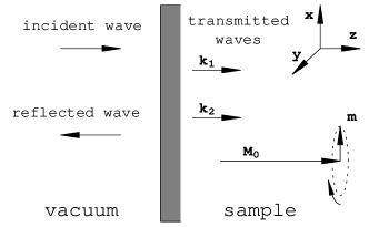
Figure 1: The setup in the perpendicular geometry.

III.1 Zero applied field

In this regime, $\mathbf{B}_{0}=0$ and $\mathbf{m_{\perp}}=\mathbf{m}$, so from Eq. (6) the spectrum of spin waves is

$$\Omega=\pm\left(\alpha+\gamma^{2}k^{2}-\frac{4\pi k^{2}\lambda^{2}}{1+k^{2}\lambda^{2}}\right)~{}.$$ (7)

The spin-wave modes are circularly polarized, and the two signs above correspond to two senses of the polarization: $\mathbf{m}^{(\pm)}=m^{(\pm)}(\mathbf{\hat{x}}\mp i\mathbf{\hat{y}})$. The polarization is determined by the incident electromagnetic radiation due to continuity of the fields across the slab surface. Only positively polarized waves can propagate inside the sample, and further on we mainly focus on this polarization. Depending on the ratio $\epsilon=\gamma/\lambda$, the spectrum can take two different forms, as shown in Fig. 2: if $\epsilon>\sqrt{4\pi}$ (high stiffness, strong superconductivity), the spectrum has a minimum (threshold for spin wave propagation) $\Omega_{f}=\alpha$ situated at $k=0$. In the opposite case, the minimum frequency is at a finite wave vector $k_{m}=\lambda^{-1}(\sqrt{4\pi}/\epsilon-1)^{1/2}$ and has a lower value $\Omega_{m}=\alpha-(\sqrt{4\pi}-\epsilon)^{2}$. In this regime, waves with wave vectors satisfying $|k|<k_{m}$ have negative group velocity $d\omega(k)/dk$. In order to carry the energy away from the boundary, these waves should have wave vectors directed toward the boundary.

For given frequency and polarization, two spin-wave modes with different wave vectors are excited by the incident radiation. For each mode, the corresponding electric and magnetic fields inside the sample are found from the Maxwell equation $\partial\mathbf{b}/\partial t=-c\mathbf{\nabla}\times\mathbf{e}$ and the London equation (4):

$$\mathbf{h} = \mathbf{b}-4\pi\mathbf{m}=-\frac{4\pi}{1+k^{2}\lambda^{2}}\mathbf{m}~{},$$

$$\mathbf{e} = \frac{\omega}{kc}\mathbf{b}\times\mathbf{\hat{z}}=\frac{\omega\lambda}{c}\frac{4\pi k\lambda}{1+k^{2}\lambda^{2}}\mathbf{m}\times\mathbf{\hat{z}}~{}.$$ (8)

The total fields are given by superposition of different modes.

Figure 2: The spin-wave spectrum in the perpendicular geometry in two regimes: stiff, $\epsilon=\sqrt{4\pi}+0.2$, $\alpha=4\pi+50$ (dashed line) and soft, $\epsilon=\sqrt{4\pi}-2.35$, $\alpha=4\pi+0.013$ (solid line).

In order to find a proper superposition of the two spin-wave modes inside the sample, an extra boundary condition is needed, in addition to the usual continuity of tangential components of the electromagnetic field at the sample surface. This additional condition should be imposed on the magnetization. The simplest possible boundary condition akhi is $\partial\mathbf{m}(z)/\partial z=0$ on the surface, which physically means absence of spin currents through the sample surface. In the Fourier space this condition gives

$$k_{1}\mathbf{m}_{1}+k_{2}\mathbf{m}_{2}=0~{}.$$ (9)

This equation together with Eq. (III.1) formulates the boundary problem, from which all fields in the slab can be found.

Now we turn to calculation of the microwave response, which is quantitatively expressed by the surface impedance and whose real part is proportional to the energy absorption by the system. LL6 For circularly polarized fields, it is given by

$$\zeta^{(\pm)}=\pm i\frac{e^{(\pm)}(z=0)}{h^{(\pm)}(z=0)}~{}.$$ (10)

Using Eqs. (III.1) and (9), we obtain, after simplification

$$\zeta^{(\pm)}=-\frac{\omega\lambda}{c}\frac{q_{1}q_{2}(q_{1}+q_{2})}{1+q_{1}^{2}+q_{2}^{2}+q_{1}q_{2}},$$ (11)

where $q_{i}=k_{i}\lambda$. Then, using the dispersion relation, Eq. (7), one can solve for the wave vectors and obtain a general expression for the surface impedance as a function of the frequency:

$$\zeta^{(\pm)}(\omega)=-\frac{\omega\lambda}{c}\frac{Q\sqrt{\pm\Omega-\delta\alpha-\epsilon^{2}+2\epsilon Q}}{\pm\Omega-\delta\alpha+\epsilon Q},$$ (12)

where $Q=i\sqrt{\pm\Omega-\alpha}$. It can be observed that $\zeta^{(-)}$ is pure imaginary since spin waves with negative circular polarization cannot propagate, and it shows regular behavior without special features. On the other hand, for the positive polarization, the impedance has a real part satisfying the inequality $\mathrm{Re}\,\zeta^{(+)}\geq 0$, as it should, and similar to the spectrum, it shows a qualitatively different behavior in the two regimes depending on the value of $\epsilon$ as can be seen in Fig. 3.

Figure 3: $\mathrm{Re}\,\zeta^{(+)}$ for the perpendicular geometry in the stiff regime, $\epsilon=\sqrt{4\pi}+0.7$ (dashed line) and soft regime, $\epsilon=\sqrt{4\pi}-1.7$ (solid line). In both cases, $\alpha=4\pi+0.2$.

Most importantly, it has several singular points (thresholds) related to spin-wave propagation properties, which can be especially useful for comparison with experiments. Below we list these points and analyze the behavior of $\zeta^{(+)}$ around them.

(i) The case $\epsilon>\sqrt{4\pi}$ (stiff spin system). Then $\Omega(k)$ is a growing function and the threshold frequency for spin-wave propagation is $\Omega_{f}=\alpha$. This frequency corresponds to uniform oscillations in SCFM, at which the electric field vanishes inside the sample. Near $\Omega_{f}$ one wave vector is small ($k_{1}\propto\sqrt{\Omega-\Omega_{f}}$), and then the surface impedance can be simplified:

$$\zeta^{(+)}\simeq\frac{\omega_{f}\lambda}{c}\frac{\sqrt{(\epsilon^{2}-4\pi)(\Omega-\Omega_{f})}}{4\pi}.$$ (13)

Thus, $\mathrm{Re}\zeta^{(+)}$ is zero below the threshold $\Omega_{f}$ and has a square-root behavior above it

(ii) The case $\epsilon<\sqrt{4\pi}$ (soft spin system). In this regime the threshold frequency has a lower value $\Omega_{m}=\alpha-(\sqrt{4\pi}-\epsilon)^{2}<\Omega_{f}$. At this frequency the electric field on the sample surface vanishes (but unlike at $\Omega_{f}$, it is nonzero inside the sample). Near $\Omega_{m}$, the two wave vectors are close in absolute value to $k_{m}$, but oppositely directed: $k_{1}+k_{2}\propto\sqrt{\Omega-\Omega_{m}}$. Then the impedance is

$$\zeta^{(+)}\simeq\frac{\omega_{m}\lambda}{c\,\epsilon}\sqrt{\frac{\sqrt{4\pi}-\epsilon}{\sqrt{4\pi}}}\sqrt{\Omega-\Omega_{m}}.$$ (14)

Thus, $\mathrm{Re}\zeta^{(+)}$ has a square-root singularity at $\Omega_{m}$.

In addition, there is still a singularity at $\Omega_{f}$. The behavior there, however, is different than in the stiff case: namely, $\mathrm{Re}\,\zeta^{(+)}$ is nonzero both above and below $\Omega_{f}$. In order to obtain it, Eq. (13) is not sufficient, and one has to go to the next order of smallness. Then

$$\zeta^{(+)}\simeq\frac{\omega_{f}\lambda}{c}\frac{\sqrt{4\pi-\epsilon^{2}}}{4\pi}\left[\frac{\epsilon^{3}(\Omega-\Omega_{f})}{4\pi(4\pi-\epsilon^{2})}-i\sqrt{\Omega-\Omega_{f}}\right],$$ (15)

so for a soft spin system, $\mathrm{Re}\,\zeta^{(+)}$ vanishes at $\Omega_{f}$, showing a square-root behavior below it and a linear one above it.

In addition to these points, where the impedance vanishes, there is a frequency $\Omega_{h}=\delta\alpha-\epsilon^{2}/2+\epsilon\sqrt{4\pi+\epsilon^{2}/4}$ at which $\zeta^{(+)}$ has a pole for both stiff and soft regimes:

$$\zeta^{(+)}\simeq\frac{i\omega_{h}\lambda}{c}\frac{(\alpha-\Omega_{h})\sqrt{\epsilon^{2}+\epsilon\sqrt{\alpha-\Omega_{h}}}}{(\sqrt{\alpha-\Omega_{h}}+\epsilon/2)(\Omega-\Omega_{h})}.$$ (16)

Then $\mathrm{Re}\,\zeta^{(+)}$ has a $\delta$-function peak at $\omega_{h}$ which acquires a finite width if small dissipation is added to the system. This peak corresponds to the ferromagnetic resonance for a SCFM slab, and it is also related to the surface wave supported by the system, whose branch starts at the same frequency $\omega_{h}$ in the limit of infinite light velocity. SW Indeed, the oscillation excited at this frequency by an incident radiation is identical to the oscillation produced in the slab by the long-wave surface wave. Finally, at large frequencies $\Omega>>\alpha$ the magnetic properties stop playing a role and the surface impedance becomes just the impedance of a plain superconductor, $\zeta=-i\omega\lambda/c$, with the real part being a small correction $\sim\omega^{-3/2}$.

Our analysis can be easily generalized to take into account dissipation due to normal currents. For this, normal current $J_{n}=\sigma_{n}E$ should be added to the superconducting current in the Maxwell equations. Here $\sigma_{n}$ is the normal conductivity and the frequencies are assumed to be not very high, so the dispersion of the conductivity can be neglected. As a result, in the London equation (4), a renormalized complex $\lambda_{n}$ should be used instead of the London penetration depth: clem

$$\lambda_{n}^{-2}=\lambda^{-2}-2i\delta^{-2},$$ (17)

where $\delta=c/\sqrt{2\pi\sigma_{n}\omega}$ is the skin depth. Consequently, the spin-wave spectrum and the surface impedance are obtained from Eqs. (7), (11), and (12) by analytic continuation using complex $\lambda_{n}$ and $\epsilon$. Then, in general, the distinction between the soft and stiff cases disappears, as $\mathrm{Re}\,\zeta^{(+)}$ loses its singularities and becomes nonzero at all frequencies, except at $\omega_{f}$, where it shows a square-root behavior both above and below $\omega_{f}$. However, if the normal currents are small, as happens in a superconductor, $\zeta$ behaves approximately in the same way as in the nondissipative situation discussed above, with the singularities smeared by a small amount $\sim\lambda^{2}\delta^{-2}$. In particular, the peak at $\omega_{h}$ acquires a finite width and can be observed.

The opposite limit $\lambda\rightarrow\infty$ and $\lambda_{n}^{2}=i\delta^{2}/2$ corresponds to a metallic ferromagnet. In this case $\mathrm{Re}\,\zeta$ again shows no features (except vanishing at $\omega_{f}$). If, however, the conductivity is not very high, $\gamma<<\delta$, then the frequencies $\omega_{h}$ and $\omega_{m}$ (calculated with a complex $\epsilon=\gamma/\lambda_{n}$) merge and the impedance shows a sharp peak there (with width $\sim\gamma/\delta$). This property has been widely used in ferromagnetic resonance measurements in metals. akhi ; Ament Thus, superconductivity modifies the microwave response in a qualitative way, which can be used for detection of the superconducting transition.

Finally, we would like to make the following comment. By analogy with metals, one might think that the limit $\lambda\to\infty$ corresponds to an insulating ferromagnet. This is not so, since in the description of the latter retardation effects are important and should be taken into account. Accordingly, the correct limit describing a magnetic insulator is $\lambda^{-2}\to-(\omega/c)^{2}$.

III.2 Finite applied field

When a finite magnetic field $B_{0}<<H_{c2}$ is applied perpendicular to the sample surface, it penetrates the sample, where the vortex phase is formed. In the presence of vortices the London equation is modified since the equation for the superconducting current density $\mathbf{j}_{s}$ now becomes

$$\frac{4\pi\lambda^{2}}{c}\nabla\times\mathbf{j}_{s}=B_{0}\frac{\partial\mathbf{u}}{\partial z}-\mathbf{b},$$ (18)

where $\mathbf{u}$ is the local displacement of the vortices from the equilibrium position. To complete the description of the problem in this regime, one needs also an equation for the vortex dynamics. The simplest reasonable model is that the vortex motion is governed by a balance of the Lorentz force and a viscous drag. In the presence of normal currents, one should be careful about the form of the Lorentz force, so that the Onsager relations are not violated. Placais A plausible assumption is that the Lorentz force depends only on the superconducting current density. With all these considerations taken into account, the vortex dynamics is described by

$$\eta\frac{\partial\mathbf{u}}{\partial t}=\frac{\Phi_{0}}{c}\mathbf{j}_{s}\times\mathbf{\hat{z}}$$ (19)

where $\eta$ is the viscous drag coefficient. Substituting this equation in the previous one, we obtain

$$\frac{4\pi\lambda_{v}^{2}}{c}\,\mathbf{\hat{z}}\times\frac{\partial\mathbf{j}_{s}}{\partial z}=-\mathbf{b},$$ (20)

where $\lambda_{v}^{2}=\lambda^{2}+iB_{0}\Phi_{0}/4\pi\omega\eta$. This equation formally coincides with the London equation in the Meissner state, so in our approximations the presence of vortices amounts to a replacement of the London penetration depth $\lambda$ by the complex $\lambda_{v}$. Then the presence of normal currents is taken into account by a further replacement Placais $\lambda_{v}^{-2}\to\lambda_{nv}^{-2}=\lambda_{v}^{-2}-2i\delta^{-2}$.

In addition, it is evident from Eq. (3) that instead of the bare anisotropy parameter $\alpha$ a modified $\tilde{\alpha}=\alpha+B_{0}/4\pi M_{0}$ should be used. Thus, the effect of the applied field is: (i) to shift the position of singularities in the response (this can be useful since it allows to take measurements at constant frequency by scanning the applied field) and (ii) to add dissipation to the system, smearing the singularities and eventually pushing the response into the metallic regime.

IV Parallel geometry

Now we consider a situation when the easy axis is parallel to the sample surface, as shown in Fig. 4. The direction perpendicular to the surface is chosen to be $\mathbf{\hat{x}}$, along which all quantities vary, and then $\mathbf{m_{\perp}}=\mathbf{\hat{y}}\,m_{y}$. Again we start from a simpler case when the magnetic induction vanishes inside the sample, $B_{0}=0$. After that, we consider a more complicated case when there is a nonzero induction near the sample surface, decaying in the bulk.

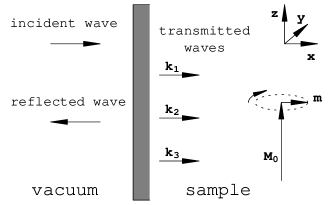
Figure 4: The setup in the parallel geometry.

IV.1 Zero static induction

The regime in which the static magnetic induction vanishes inside the sample can be realized by application of an external field $\mathbf{H}_{0}=-4\pi\mathbf{M}_{0}$. Strictly speaking, this configuration is not stable, since flipping $\mathbf{M}_{0}$ in the opposite direction would lower the energy. However, it is metastable provided the anisotropy is strong enough, $\alpha>4\pi$. From Eq. (6) the spectrum of spin waves now is

$$\Omega^{2}=\left(\alpha+\gamma^{2}k^{2}\right)\left(\alpha+\gamma^{2}k^{2}-\frac{4\pi k^{2}\lambda^{2}}{1+k^{2}\lambda^{2}}\right).$$ (21)

It can be seen from this relation that in the parallel geometry an incident electromagnetic wave excites in the sample three spin-wave modes. Since the dynamical part of the magnetization has only one component in the plane of the sample surface, $m_{y}$, the spin wave in this geometry is excited by a linearly polarized incident radiation with the magnetic component in the $\mathbf{\hat{y}}$ direction. The spectrum has the same qualitative features as in the perpendicular geometry, although the specific values of different parameters are, of course, different. Thus, the transition between the soft and stiff regimes occurs now at $\epsilon=\sqrt{2\pi}$, while the wave vector $k_{m\,\parallel}$ and the frequency $\omega_{m\,\parallel}$ can be found by minimizing Eq. (21), which requires solution of a cubic equation. Note, however, that the frequency of uniform oscillations $\Omega_{f}$ remains equal $\alpha$ in this geometry.

The boundary condition, Eq. (9), now gives two independent equations for $\mathbf{\hat{x}}$ and $\mathbf{\hat{y}}$ components of the magnetization. These two components are related by Eq. (6):

$$i\Omega\,m_{y}=(\alpha+\gamma^{2}k^{2})m_{x}.$$ (22)

Using this, the boundary conditions can be written as

$$\sum k_{i}\,m_{x\,i}=0$$

$$\sum k_{i}^{3}\,m_{x\,i}=0,$$ (23)

where the summation is over the three spin-wave modes. These conditions determine the relative amplitudes of the modes and together with the dispersion relation specify the problem completely.

The surface impedance for this case of linearly polarized incident wave is given by

$$\zeta=-\frac{e_{z}(x=0)}{h_{y}(x=0)}.$$ (24)

Then the calculation goes along the same steps as for the perpendicular geometry, though it is more complicated due to the presence of three modes. Using Eqs. (III.1), (22), and (IV.1), one obtains, after some algebra,

$$\zeta=\frac{\omega\lambda}{c}\,\frac{a_{2}(a_{1}a_{3}-a_{2})\epsilon^{4}}{a_{1}(\Omega^{2}-\alpha\,\delta\alpha)+a_{2}[(2\alpha-4\pi)\epsilon^{2}-a_{3}\epsilon^{4}]},$$ (25)

where $a_{j}$ are symmetric combinations of the normalized wave vectors for different modes (and, as before, $q_{i}=k_{i}\lambda$):

$$a_{1} = q_{1}+q_{2}+q_{3},$$

$$a_{2} = q_{1}q_{2}q_{3},$$

$$a_{3} = q_{1}q_{2}+q_{2}q_{3}+q_{3}q_{1}.$$ (26)

These combinations can be found from the dispersion relation, Eq. (21), thus providing the dependence of $\zeta$ on the frequency. As can be seen from Fig. 5, $\mathrm{Re}\,\zeta$ shows the same qualitative behavior as in the perpendicular geometry around its singularities. The same is also true about the high-frequency behavior of $\zeta$, given by $-i\omega\lambda/c$ with a small real correction $\sim\omega^{-3/2}$. Below we give expressions for $\zeta$ near the propagation thresholds.

Figure 5: $\mathrm{Re}\,\zeta$ for the parallel geometry in the stiff regime, $\epsilon=\sqrt{2\pi}+0.1$ (dashed line) and soft regime, $\epsilon=\sqrt{2\pi}-1.$ (solid line). In both cases, $\alpha=4\pi+0.3$.

(i) In the stiff regime $\epsilon>\sqrt{2\pi}$, the impedance near the threshold $\Omega_{f}=\alpha$ shows a square-root singularity

$$\zeta\simeq\frac{\omega_{f}\lambda}{c}\frac{\sqrt{(\epsilon^{2}-2\pi)(\Omega-\Omega_{f})}}{2\pi}$$ (27)

(ii) In the soft regime $\epsilon<\sqrt{2\pi}$, the threshold is at $\omega_{m\,\parallel}$, again with a square-root behavior around it:

$$\zeta \simeq \frac{\omega_{m\,\parallel}\lambda}{c}\frac{q_{m\,\parallel}(\alpha-\epsilon^{2})\sqrt{3\epsilon^{2}q_{m\,\parallel}^{2}+2\alpha-4\pi+\epsilon^{2}}}{2\epsilon(\alpha+\epsilon^{2}q_{m\,\parallel}^{2})(\epsilon^{2}q_{m\,\parallel}^{2}+\alpha-2\pi)\sqrt{1+q_{m\,\parallel}^{2}}}$$ (28)

$$\times\sqrt{\Omega^{2}-\Omega_{m\,\parallel}^{2}}.$$

Finally, Eq. (25) has a pole at a frequency $\omega_{h\,\parallel}$, at which $\mathrm{Re}\zeta$ shows a peak, just like in the perpendicular geometry.

IV.2 Finite static induction

If the applied magnetic field $\mathbf{H}_{0}$(parallel to the surface) is not exactly equal to $-4\pi\mathbf{M}_{0}$, then there is a nonzero magnetic induction penetrating the sample,

$$\mathbf{B}_{0}(x)=(4\pi\mathbf{M}_{0}+\mathbf{H}_{0})e^{-x/\lambda}.$$ (29)

In this case the translational invariance of the system is broken, so the spin-wave modes are not plane waves anymore. This considerably complicates the problem, since these modes are given, instead of Eq. (21), by a sixth-order differential equation

$$\Omega^{2}(\lambda^{-2}-\partial_{x}^{2})m_{x}=(\lambda^{-2}-\partial_{x}^{2})(\alpha+fe^{-x/\lambda}-\gamma^{2}\partial_{x}^{2})^{2}m_{x}$$

$$+4\pi\partial_{x}^{2}(\alpha+fe^{-x/\lambda}-\gamma^{2}\partial_{x}^{2})m_{x},$$ (30)

where $f=(4\pi+H_{0}/M_{0})$ is the magnetic induction at the sample surface divided by $M_{0}$. Then the general solution of the problem including finding the modes, matching them by the boundary conditions, and calculating the surface impedance would be very difficult. Instead of this we limited our attention to two extreme regimes in which the problem can be simplified. Namely, we considered the regime of very low stiffness (very soft regime), $\epsilon<<1$, and the opposite very stiff regime $\epsilon>>1$. In the former case, the Meissner layer is wide and the static magnetic field there is very smooth, and therefore the quasiclassical approximation can be applied; in the latter, the Meissner layer is extremely thin and its influence is weak.

IV.2.1 Very soft regime

In this regime $\epsilon<<1$, and the dispersion of free spin-wave modes (those outside of the Meissner layer) can be obtained by simplification of Eq. (21):

$$\Omega^{2}=(\alpha+\gamma^{2}k^{2})(\delta\alpha+\gamma^{2}k^{2})+\frac{4\pi}{1+k^{2}\lambda^{2}}.$$ (31)

Then the threshold frequency $\Omega_{m\,\parallel}$ for spin-wave penetration is given by

$$\Omega_{m\,\parallel}^{2}=\alpha\delta\alpha+4\epsilon\sqrt{2\pi\alpha(\alpha-2\pi)}+O(\epsilon^{2})$$ (32)

and the corresponding wave vector is

$$k_{m}=\frac{1}{\sqrt{\gamma\lambda}}\sqrt[4]{\frac{2\pi\alpha}{\alpha-2\pi}}.$$ (33)

Of the three spin-wave modes corresponding to a general frequency $\Omega$, two have short wavelength $\sim\gamma$, while one has long wavelength $\lambda$. However, for frequencies near $\Omega_{m\,\parallel}$, the picture changes: namely, one has a short-wave decaying mode with $k_{3}^{2}=-2(\alpha-2\pi)\gamma^{-2}$ and two modes with intermediate wavelengths $\sim\sqrt{\gamma\lambda}$. Since in this case all wavelengths are much shorter than the scale of variation of the “potential” [provided by the field $\mathbf{B}_{0}(x)$], it is possible to treat the spin-wave equation (IV.2) by the quasiclassical approximation (its validity is discussed below in more detail).

Thus we will be interested in finding $\zeta$ (and in particular, its real part) for frequencies slightly above the threshold, $0<\Omega-\Omega_{m\,\parallel}\sim\epsilon$ and in the presence of weak magnetic induction $B_{0}\sim\epsilon M_{0}$ directed either parallel or antiparallel to $\mathbf{M}_{0}$. We start by discussing $\zeta$ in the absence of $B_{0}$. From the free-wave spectrum, Eq. (31), one finds relations between the wave vectors $k_{1}$ and $k_{2}$:

$$k_{1}^{2}+k_{2}^{2}=\frac{\Omega^{2}-\alpha\delta\alpha}{2(\alpha-2\pi)}\gamma^{-2},$$

$$k_{1}^{2}k_{2}^{2}=\frac{2\pi\alpha}{\alpha-2\pi}\gamma^{-4}\lambda^{-2},$$ (34)

while the short-wave-mode wave vector $k_{3}$ has been specified earlier. From these relations it is not difficult to find the wave vectors and substitute them into Eq.  (25), thus obtaining

$$\zeta=\frac{\omega_{m\,\parallel}\lambda}{c}\frac{\sqrt{4\pi\alpha}\sqrt{\Omega^{2}-\Omega_{m\,\parallel}^{2}}}{\Omega^{2}-\Omega_{h\,\parallel}^{2}},$$ (35)

where the resonance frequency $\Omega_{h\,\parallel}$ is given (in the very soft regime) by

$$\Omega_{h\,\parallel}^{2}=\alpha\delta\alpha+2\epsilon\sqrt{2\pi\alpha(\alpha-2\pi)}.$$ (36)

We recall that Eq. (35) is valid only near $\omega_{m\,\parallel}$, where Eqs. (IV.2.1) hold. To lowest order in $\omega-\omega_{m\,\parallel}$, Eq. (35) reduces to

$$\zeta=\frac{\omega_{m\,\parallel}\lambda}{c}\frac{\sqrt{\Omega_{m\,\parallel}(\Omega-\Omega_{m\,\parallel})}}{\epsilon\sqrt{\alpha-2\pi}},$$ (37)

which coincides with Eq. (28) in the very soft ($\epsilon<<1$) limit.

Let us now turn on the magnetic induction $\mathbf{B}_{0}(x)$; then, its presence can be effectively described by an $x$-dependent anisotropy factor $\alpha(x)=\alpha+B_{0}(x)/M_{0}$. According to the quasiclassical approximation, the corresponding spin-wave modes are found from the free modes by using $x$-dependent wave vectors. Note that for the short-wave mode 3 this dependence can be neglected since it is small and regular. On the other hand, for the modes 1 and 2, this dependence is crucial, since it determines properties of the wave propagation such as tunnelling. Indeed, substituting $\alpha(x)$ into Eq. (32), one obtains the $x$-dependent threshold frequency

$$\Omega_{m\,\parallel}^{2}(x)=\Omega_{m\,\parallel}^{2}+2(\alpha-2\pi)fe^{-x/\lambda},$$ (38)

which can be considered as an effective potential as shown in Fig. 6. In the region where $\Omega>\Omega_{m\,\parallel}(x)$, modes 1 and 2 are propagating, while if $\Omega<\Omega_{m\,\parallel}(x)$, these modes can only tunnel under the potential barrier. The point $x_{T}$ between these two regions is a classical turning, or reflection point. It is defined by the condition

$$\Omega=\Omega_{m\,\parallel}(x_{T}).$$ (39)

The field-free threshold $\Omega_{m\,\parallel}=\Omega_{m\,\parallel}(x=\infty)$ remains the propagation threshold so that only radiation with $\Omega>\Omega_{m\,\parallel}$ can penetrate (here we ignore the peak at $\omega_{h\,\parallel}$). When $B(x)<0$, this penetration is classically possible, since $\Omega>\Omega_{m\,\parallel}(x)$, while when $B(x)$ is positive and not too small, so that $\Omega_{m\,\parallel}(0)>\Omega$, it is realized by tunneling.

Figure 6: Coordinate-dependent threshold frequency $\omega_{m\,\parallel}(x)$ serving as an effective potential for $B_{0}>0$ (solid line) and $B_{0}<0$ (dashed line).

The validity of the quasiclassical approximation is of special concern in this problem. Indeed, as was mentioned above, one can hope to use the quasiclassics only near the threshold $\Omega_{m\,\parallel}$. On the other hand, $\Omega_{m\,\parallel}(x)=\Omega$ means that the motion is near the turning point, around which the quasiclassics breaks down. The usual condition of validity $\partial_{x}k(x)<<k^{2}$, is not sufficient here, since, unlike in quantum mechanics, the turning point corresponds not to zero but a finite wave vector $k_{m}$ so that $\Omega(k)-\Omega_{m\,\parallel}\propto(k-k_{m})^{2}$ (for the mode with $\mathrm{Re}\,k>0$). Instead, a more stringent condition is required,

$$\frac{\partial\,\delta k}{\partial x}<<\delta k^{2},$$ (40)

where $\delta k=k-k_{m}$. There is also another dangerous frequency given by $\Omega_{-}^{2}=\alpha\delta\alpha-4\epsilon\sqrt{2\pi\alpha(\alpha-2\pi)}$, at which $k^{2}=-k_{m}^{2}$, the group velocity vanishes and the quasiclassics breaks down again (this frequency has no quantum-mechanical counterpart). However, it is situated deep inside the classically forbidden region, and we ignore it, assuming $\Omega$ to be always larger than it. Then the above condition reduces to

$$\epsilon fe^{-x/\lambda}<<\left|\frac{\Omega^{2}-\Omega_{m\,\parallel}^{2}(x)}{\alpha-2\pi}\right|^{3/2}.$$ (41)

(i) For $B(x)<0$, the effective potential bends down. Then, as long as the quasiclassics holds, the wave propagation inside is described by two outgoing modes 1 and 2 (plus the evanescent short-wave mode 3) with $x$-dependent wave vectors found from Eq. (IV.2.1). Then $\zeta$ can be calculated exactly as in the field-free case, but with a local value of $\alpha$ at the surface, $\alpha(x=0)=\alpha+f$. The result is

$$\zeta=\frac{\omega_{m\,\parallel}\lambda}{c}\frac{\sqrt{4\pi\alpha}\sqrt{\Omega^{2}-\Omega_{m\,\parallel}^{2}-2(\alpha-2\pi)f}}{\Omega^{2}-\Omega_{h\,\parallel}^{2}-2(\alpha-2\pi)f},$$ (42)

which has just the field-free form shifted to the left ($f<0$). One might worry about this result that it gives real $\zeta$ for $\Omega<\Omega_{m\,\parallel}$. In fact, as $\Omega\to\Omega_{m\,\parallel}$, the quasiclassics breaks down at some depth inside the slab, and this result loses its validity. This is expressed in the appearance of significant over-barrier reflection. Then the correct frequency dependence becomes $\mathrm{Re}\zeta\propto\sqrt{\Omega-\Omega_{m\,\parallel}}$. However, as long as $\Omega$ is not too close to $\Omega_{m\,\parallel}$ [e.g., for $f\sim\Omega-\Omega_{m\,\parallel}\sim\epsilon$, when condition (41) is satisfied for any $x$], the result given above is valid.

(i) For $B(x)>0$, the effective potential bends up, forming a barrier. For frequencies $\Omega_{m\,\parallel}<\Omega<\Omega_{m\,\parallel}(0)$, the wave penetration is realized by tunneling of the modes 1 and 2, which means that each of these modes consists of a dominant decreasing part and a small (subdominant) increasing part (while the mode 3 remains unaffected). The tunneling occurs until the turning point $x_{T}$, after which the modes become propagating. In order to calculate $\mathrm{Im}\,\zeta$, one may neglect the tunneling, thus assuming that all the energy is reflected from the barrier. Then only the dominant part of the modes should be retained, the problem becomes again formally analogous to the free case, and $\mathrm{Im}\,\zeta$ is given by Eq. (42) with $f>0$. Calculation of $\mathrm{Re}\,\zeta$ is more difficult, since it requires higher precision. It can be done directly by keeping both the dominant and subdominant parts and solving a boundary-value problem with five components. However, it is easier to solve the problem using the fact that $\mathrm{Re}\zeta$ is proportional to the energy flux:

$$\mathrm{Re}\,\zeta=\frac{8\pi}{c}P|h_{y}(0)|^{-2}.$$ (43)

The flux may be calculated in the region after the turning point, where it is given by

$$P=\sum_{i=1,2}\frac{\omega_{m}|m_{x\,i}(x)|^{2}}{4\alpha}\frac{\partial\Omega^{2}(k[x])}{\partial k},$$ (44)

with $\Omega(k)$ given by Eq. (31). The transmitted amplitudes may be related to the amplitudes at the boundary by a procedure analogous to the quasiclassical calculation of transmission coefficient in quantum mechanics, LL3 neglecting the subdominant parts. When this is done, one has to relate different mode amplitudes at $x=0$ using the boundary conditions, Eq. (IV.1). Substituting the results into Eqs. (43) and (44), one obtains

$$\mathrm{Re}\,\zeta=\frac{8\lambda\,\omega_{m\,\parallel}}{c}\frac{\epsilon^{3/2}(\alpha-2\pi)^{3/4}(2\pi\alpha)^{5/4}\sqrt{\Omega_{m\,\parallel}^{2}(0)-\Omega^{2}}}{[\Omega^{2}-\Omega_{h\,\parallel}^{2}(0)]^{2}\sqrt{\Omega^{2}-\Omega_{-}^{2}(0)}}\,t,$$ (45)

where for all threshold frequencies, $\Omega^{2}(0)=\Omega^{2}+2(\alpha-2\pi)f$ and

$$t=\exp\left[-2\int_{0}^{x_{T}}\mathrm{Im}k(x)\,dx\right]$$ (46)

is the tunneling exponent. Using Eqs. (IV.2.1) and (39), one finds

$$t=\exp\left[-2\epsilon^{-1}\sqrt{fe^{-\xi_{T}}}\left(\sqrt{e^{\xi_{T}}-1}-\arctan\sqrt{e^{\xi_{T}}-1}\right)\right],$$ (47)

with

$$e^{\xi_{T}}=e^{x_{T}/\lambda}=2f\frac{\alpha-2\pi}{\Omega^{2}-\Omega_{m\,\parallel}^{2}}.$$ (48)

Note that $\zeta$ may have a peak of finite width if the field is strong enough so that $\omega_{h\,\parallel}(0)>\omega_{m\,\parallel}$. The peak is cut off at $\Omega^{2}-\Omega_{h\,\parallel}^{2}(0)\sim\epsilon^{3/2}t$, when the subdominant part becomes significant and the tunneling is no longer small, as was assumed. On the other hand, the singularity at $\Omega_{-}(0)$ is disregarded, since, as we mentioned above, this frequency is assumed to be always smaller than $\Omega_{m\,\parallel}$. The calculation remains valid for $\Omega$ going down to $\Omega_{m\,\parallel}$. The reason for this is that unlike in the previous case, the quasiclassics now does not need to hold everywhere in the sample (it is anyway broken around the turning point), but only in some finite region under the barrier and deep inside after $x_{T}$. It can be seen from Eq. (41) that these requirements are satisfied for $0<\Omega-\Omega_{m\,\parallel}\lesssim f\sim\epsilon$. Plots of $\mathrm{Re}\,\zeta$ for $B_{0}=0,B_{0}<0,$ and $B_{0}>0$ are shown on Fig. 7. One can see that for the antiparallel field ($B_{0}<0$) the response is not affected significantly, unlike for the parallel field.

Figure 7: Effect of magnetic field in the parallel geometry, very soft regime. $\mathrm{Re}\,\zeta$ for $f=0$ (thick line), $f=0.05$ (thin solid line, its scale given to the right), and $f=-0.05$ (dashed line), which is extrapolated to have a square-root behavior near $\omega_{m}$ (dotted line). Note that the values of $\omega_{h\,\parallel}(0)$ and $\omega_{m\,\parallel}(0)$ are given for a positive field $(f=0.05)$. Parameter values for the plots are $\alpha=4\pi+1$ and $\epsilon=0.01$.

IV.2.2 Very stiff regime

In this regime $\epsilon>>1$, which corresponds to the limit of very strong superconductivity. Thus the Meissner layer is very thin, and its influence amounts to modification of the boundary conditions. The threshold for wave propagation in this regime is $\Omega_{f}=\alpha$. Again we start by considering the field-free situation first. The free spin-wave spectrum, Eq. (21), yields in this regime one short-wave and two long-wave modes:

$$k_{1}^{2}\approx-\lambda^{-2},\quad k_{2,3}^{2}\approx\gamma^{-2}(\pm\Omega-\alpha).$$ (49)

Substituting them into Eqs. (25) and (IV.1), one finds the field-free result

$$\zeta=\frac{\omega\lambda}{c}\left(-i+\frac{2\pi}{\epsilon\sqrt{\Omega-\alpha}}\right).$$ (50)

Thus to the leading order $\zeta$ is pure imaginary and corresponds to the surface impedance of a usual nonmagnetic superconductor, as it should in this regime of strong superconductivity. Note that this expression is not valid very near the threshold - namely, for $\Omega-\alpha\lesssim\epsilon^{-2}$ - and hence it does not capture the special behavior there, such as the square-root singularity $\zeta\sim\sqrt{\Omega-\alpha}$ and a pole at $\Omega_{h\,\parallel}$ (in this regime $\omega_{h\,\parallel}$ and $\omega_{f}$ are close to each other).

Now we introduce the magnetic field, Eq. (29), which is not assumed small, and calculate the change in $\mathrm{Re}\,\zeta$ due to it. As will be shown below, the change comes only as a small correction $\sim\epsilon^{-2}$ to the field-free results; hence, small terms $\sim\epsilon^{-2}$ should be retained in the calculation. To start with, it is useful to rewrite the spin-wave equation, Eq. (IV.2), in terms of a rescaled coordinate $\xi=x/\lambda$:

$$\Omega^{2}(1-\partial_{\xi}^{2})m_{x}=(1-\partial_{\xi}^{2})(\alpha+fe^{-\xi}-\epsilon^{2}\partial_{\xi}^{2})^{2}m_{x}$$

$$+4\pi\partial_{\xi}^{2}(\alpha+fe^{-\xi}-\epsilon^{2}\partial_{\xi}^{2})m_{x}.$$ (51)

This equation contains a large parameter $\epsilon$, which makes it possible to find the solutions as an expansion in $\epsilon^{-1}$. As in the field-free case, one has a short-wave mode

$$m_{x\,1}(\xi)\approx m_{1}e^{-\xi}\left(1+\frac{5f}{16}\epsilon^{-2}e^{-\xi}\right)$$ (52)

and two long-wave modes

$$m_{x\,\,2,3}(\xi)\approx m_{2,3}\exp(iq_{2,3}\xi)(1+f\epsilon^{-2}e^{-\xi}),$$ (53)

where we have only retained corrections related to the field ($\sim f$). Similarly one finds the modes for $m_{y}$,

$$m_{y\,1}(\xi)=-\epsilon^{2}\frac{m_{1}e^{-\xi}}{i\Omega}\left(1+\frac{f\epsilon^{-2}e^{-\xi}}{4}\right),$$

$$m_{y\,\,2,3}(\xi)=\mp im_{2,3}\exp(iq_{2,3}\xi)(1+\epsilon^{-2}fe^{-\xi}),$$ (54)

where in the second equation the upper sign is used for mode 2 and lower for mode 3, and analogously for $b_{y}$,

$$b_{y\,1}(\xi)=\epsilon^{4}\frac{m_{1}e^{-\xi}}{i\Omega},$$

$$b_{y\,2,3}(\xi)=\mp 4\pi im_{2,3}\exp(iq_{2,3}\xi)\left(q_{2,3}^{2}-\frac{\epsilon^{-2}fe^{-\xi}}{2iq_{2,3}}\right),\quad$$ (55)

and $h_{y}$,

$$h_{y\,1}(\xi)=\frac{\epsilon^{4}m_{1}e^{-\xi}}{i\Omega}$$

$$h_{y\,2,3}(\xi)=\pm 4\pi im_{2,3}\exp(iq_{2,3}\xi)\left(1+\frac{\epsilon^{-2}fe^{-\xi}}{2iq_{2,3}}\right).\quad$$ (56)

Now one should use the boundary conditions in order to relate the amplitudes of different modes. It would be incorrect to use the conditions $\nabla\mathbf{m}(0)$ directly since differentiation would reduce the relative precision in the long-wave modes and the result would only have a precision of $\epsilon^{-1}$. Instead, one should integrate the equations for magnetization components, Eq. (3), over the Meissner layer and use the above condition in the integral of $\nabla^{2}\mathbf{m}$, leading to

$$\int[fe^{-\xi}m_{y}(\xi)-b_{y}(\xi)]\,\mathrm{d}x=\epsilon^{2}(q_{2}m_{2}-q_{3}m_{3}),$$

$$\int fe^{-\xi}m_{x}(\xi)\,\mathrm{d}x=\epsilon^{2}(iq_{2}m_{2}+iq_{3}m_{3}).$$ (57)

Substituting the expressions for the magnetization components and $b_{y}$, one obtains relations between the mode amplitudes:

$$\frac{\epsilon^{2}}{\Omega}m_{1}\left(1+\frac{\epsilon^{-2}f}{2}\right)=$$

$$\quad\sum_{j=2,3}\pm m_{j}\left(-iq_{j}+\epsilon^{-2}f(1+iq_{j})+2\pi\frac{\epsilon^{-4}f}{iq_{j}}\right)$$

$$m_{2}(iq_{2}-\epsilon^{-2}f)+m_{3}(iq_{3}-\epsilon^{-2}f)=0,$$ (58)

where again the upper and lower signs in the first equation refer to modes 2 and 3, respectively. These relations are used in an expression for the energy flux in the region deeper than the Meissner layer,

$$P=\omega\lambda\epsilon^{2}|m_{2}|^{2}\mathrm{Re}\,q_{2}$$ (59)

(where only mode 2 contributes as it is the only propagating mode), and in Eq. (IV.2.2), which are subsequently substituted in Eq. (43) to calculate $\mathrm{Re}\,\zeta$. The result is

$$\mathrm{Re}\,\zeta=\frac{\omega\lambda}{c}\frac{2\pi\epsilon^{-1}}{\sqrt{\Omega-\alpha}}\left(1+3\epsilon^{-2}f+\frac{8\pi\alpha\epsilon^{-2}f}{\Omega^{2}-\alpha^{2}}-\frac{f^{2}\epsilon^{-2}}{\Omega-\alpha}\right).$$ (60)

Thus the influence of the field is given by a sum of three contributions which can be extracted by considering the frequency and field dependences of the response. All these contributions come about as small corrections $\sim\epsilon^{-2}$, although the field itself (near the surface) is not small. This is because the Meissner layer is very thin.

V Conclusions

I have considered the microwave response properties of a slab made of a material with coexisting superconductivity and magnetism and calculated its surface impedance for the parallel and perpendicular geometry. The impedance, and especially its real part, shows a rich behavior around threshold frequencies, related to spin-wave propagation. In the stiff regime, the propagation threshold is $\omega_{f}$, above which $\mathrm{Re}\,\zeta$ shows a square-root singularity. On the other hand, in the soft regime this behavior is observed near a lower threshold $\omega_{m}$, while around $\omega_{f}$, $\mathrm{Re}\,\zeta$ has a square-root singularity below it and a linear behavior above it. In addition, there is a resonance peak at $\omega_{h}$ in both regimes, related to excitation of a surface spin wave. SW The high-frequency response is mostly imaginary, being dominated by the superconductivity, with a small real correction $\sim\omega^{-3/2}$.

This behavior is common for both geometries in the field-free situation, when no magnetic induction exists at the sample surface. However, when such an induction does exist, its influence is completely different in these geometries. In the perpendicular geometry, the magnetic induction penetrates the slab in form of vortices. This leads to a change in the effective anisotropy constant, resulting in a uniform shift of all thresholds and allowing one to detect the resonances by sweeping the magnetic field at constant frequency. However, it also leads to an increased dissipation, smearing the singularities and eventually pushing the response into the metallic regime.

On the other hand, in the parallel geometry, the magnetic induction is screened inside the Meissner layer. We found the influence of the induction in the regimes of very low and very high magnetic stiffness. In the former limit the response near $\omega_{m\,\parallel}$ is strongly direction-dependent: for $\mathbf{B}$ and $\mathbf{M}_{0}$ in the opposite directions, the response is not changed significantly, while if they are parallel to each other, $\mathrm{Re}\,\zeta$ is exponentially suppressed due to a potential barrier formed in the Meissner layer. In addition, it also shows a singularity $\sim[\omega-\omega_{h\,\parallel}(0)]^{-2}$, once the induction is strong enough so that $\omega_{h\,\parallel}(0)>\omega_{m\,\parallel}$. In the opposite very stiff regime dominated by strong superconductivity, the induction is screened out very fast and its influence is weak. Interestingly, the directional dependence of the response is opposite to the previous case, so that $\mathrm{Re}\zeta(B_{0}>0)>\mathrm{Re}\zeta(B_{0}<0)$.

These results demonstrate that the magnetic and superconducting properties of SCFM’s (including unconventional superconductors with orbital magnetism) can be effectively investigated by microwave response measurements and provide a theoretical basis for such experiments.

- (1) I. Felner, U. Asaf, Y. Levi, and O. Millo, Phys. Rev. B55, 3374 (1997); E. B. Sonin and I. Felner, ibid 57, R14000 (1998); C. Bernhard, J. L. Tallon, Ch. Niedermayer, Th. Blasius, A. Golnik, E. Brücher, R. K. Kremer, D. R. Noakes, C. E. Stronach, and E. J. Ansaldo, ibid 59, 14099 (1999).
- (2) G. M. Luke, Y. Fudamoto, K. M. Kojima, M. I. Larkin, J. Merrin, B. Nachumi, Y. J. Uemura, Y. Maeno, Z. Q. Mao, Y. Mori, H. Nakamura, and M. Sigrist, Nature (London), 394, 558 (1998).
- (3) C. Pfleiderer, M. Uhlarz, S. M. Hayden, R. Vollmer, H. von Lohneysen, N. R. Bernhoeft, and G. G. Lonzarich, Nature (London) 412, 58 (2001).
- (4) S. S. Saxena, P. Agarwal, K. Ahilan, F. M. Grosche, R. K. W. Haselwimer, M. J. Steiner, E. Pugh, I. R. Walker, S. R. Julian, P. Monthoux, G. G. Lonzarich, A. Huxley, I. Sheikin, D. Braithwaite, and J. Flouqet, Nature (London) 406, 587 (2000).
- (5) A. Fainstein, E. Winkler , A. Butera, and J. Tallon, Phys. Rev. B60, R12597 (1999); N. O. Moreno, P. G. Pagliuso, J. C. P. Campoy, E. Granado, C. Rettori, S.-W. Cheong, and S. B. Oseroff, Phys. Status Solidi B 220, 541 (2000); M. Požek, A. Dulčič, D. Paar, G. V. M. Williams, and S. Krämer, Phys. Rev. B64, 064508 (2001).
- (6) T. K. Ng and C. M. Varma, Phys. Rev. B58, 11624 (1998).
- (7) T. K. Ng and C. M. Varma, Phys. Rev. Lett. 78, 330 (1997); 78, 3745 (1997).
- (8) V. Braude and E. B. Sonin, Phys. Rev. Lett. 93, 117001 (2004).
- (9) V. Braude and E. B. Sonin, Phys. Rev. B74, 064501 (2006).
- (10) V. Braude and E. B. Sonin, Europhys. Lett. 72, 124 (2005).
- (11) U. Krey, Int. J. Magn., 3, 65 (1972).
- (12) A. I. Akhiezer, V. G. Bar’yakhtar, and S. V. Peletminskii, Spin Waves (North-Holland, Amsterdam, 1968).
- (13) L. D. Landau and E. M. Lifshitz, Electrodynamics of Continuous Media (Pergamon Press, Oxford, 1984).
- (14) M. W. Coffey and J. R. Clem, Phys. Rev. Lett. 67, 386 (1991).
- (15) W. S. Ament and G. T. Rado, Phys. Rev. 97, 1558 (1955).
- (16) B. Plaçais, P. Mathieu, Y. Simon, E. B. Sonin, and K. B. Traito Phys. Rev. B54, 13083 (1996).
- (17) L. D. Landau and E. M. Lifshitz, Quantum Mechanics (Pergamon Press, Oxford, 1977).