Spin wave instabilities and field induced transitions in heavy fermions

Abstract

We study phase transitions in heavy fermion systems due to spin-wave instabilities. One motivation is to determine the changes in the spin-wave parameters of a magnetically ordered heavy fermion system as it approaches a quantum critical point (QCP) by applying pressure. The other more actual is to provide an alternative approach, based on spin-wave instabilities, for the magnetic field induced transitions recently observed in antiferromagnetic heavy fermion materials.

I Introduction

Pressure and magnetic field have been used as external parameters to drive heavy fermion materials through different quantum critical points review . The theory of the heavy fermion quantum criticality has been developed starting on the paramagnetic side of their phase diagram mucio . In the ordered magnetic phase, usually with antiferromagnetic (AF) long range order, most studies have concentrated in determining the shape of the critical line as a function of pressure ($P$) and magnetic field ($H$), in particular when $T_{N}\rightarrow 0$ review . This gives information on the important shift exponent which is determined by the critical exponents associated with the QCP. However, in the broken symmetry phase, the magnetic excitations are spin-waves and a relevant question concerns what happens to these modes as the quantum critical point (QCP) is approached from the ordered side suzana . More specifically, we ask what happens to the spin-wave parameters, its gap and stiffness as, for example, $T_{N}(P)$ goes to zero, i.e., $P$ approaches $P_{C}$ the critical pressure? The most direct way to answer this question would be to perform neutron scattering experiments, but these are non trivial. There are other less direct strategies to follow these modes as the system approaches a QCP. One of these is the electrical resistivity. Since magnons scatter the conduction electrons of the correlated metal, the temperature dependent resistivity has a component which is due to electron-magnon scattering. The temperature dependence of this component yields direct information on the spin-wave gap and stiffness suzana .

Recently, there have been many experimental studies on field induced transitions in magnetic heavy fermion systems fieldinduced . The analysis of these experiments takes into account correlated electrons with masses strongly renormalized by the presence of a QCP at the critical field $H_{C2}$ (see Fig.1). However, field induced magnetic transitions are associated with soft spin-wave modes. Consequently, close to $H_{C2}$ these modes give an important contribution to the thermodynamic properties and electrical resistivity, by scattering the quasi-particles. These contributions should be included in an analysis of this phase transition, besides that of other quasi-particles.

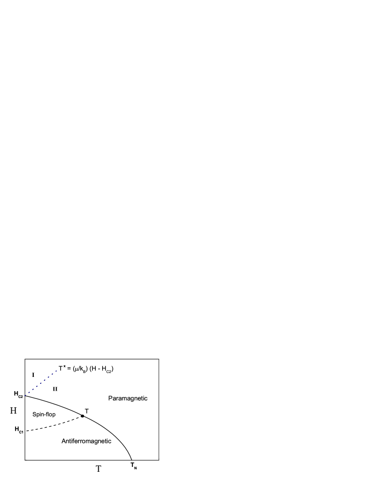
Figure 1: (Color online) Phase diagram of an anisotropic antiferromagnet in an external magnetic field in the easy axis directionkeffer . The three phases, antiferromagnet, spin-flop and paramagnetic and the tricritical point (T) are shown. The full lines are lines of second order phase transitions. The dashed line is a line of first order transitions and the dotted line is a crossover line dividing the paramagnetic region in two regimes, as explained in the text.

The magnetic field and temperature dependent phase diagram of an anisotropic antiferromagnet, with the external field $H$ applied in the easy axis direction keffer , is shown schematically in Fig.1. General features of this phase diagram are the presence of a tricritical point and lines of first and second order transitions. Heavy fermions are in general strongly anisotropic and a relevant situation for these materials is the metamagnetic case where there is no intermediate spin-flop phase at all and the system goes directly from the antiferromagnetic phase to the paramagnetic phase through a line of second order phase transitions, $H_{C2}(T)$.

II Resistivity of the anisotropic antiferromagnet in zero magnetic field

We start considering the case relevant for the study of heavy fermions systems, driven by pressure to a QCP. The spectrum of hydrodynamic spin-wave excitations in the antiferromagnetic phase, for $H<<H_{C1}$ ($T<<T_{N}$) (see Fig.1), is given by,

$$\omega(k)=-\mu H\pm\sqrt{\Delta^{2}+Dk^{2}}$$

where the gap $\Delta$ is proportional to the anisotropy (either exchange or single ion). In the isotropic case and in the absence of a magnetic field, the hydrodynamic magnons have a linear dispersion relation, $\omega(k)=\sqrt{D}k$, differently from those in a ferromagnet, for which, $\omega(k)=Dk^{2}$.

We consider first a metallic antiferromagnet in a simple cubic lattice with no applied external field. Following Yamada and Takada yamada we write the electrical resistivity due to electron-magnon scattering as,

$$\rho(T)=CI_{AF}(H=0,T)$$ (1)

where $C$ is a constant. The quantity $I_{AF}(0,T)$ is given by the following integral yamada ,

$$I_{AF}(0,T)=\frac{\beta}{2}\int_{0}^{\infty}dk\frac{k^{2}}{\sinh^{2}\frac{\beta\epsilon_{k}}{2}}$$ (2)

where $\omega(k)=\sqrt{\Delta^{2}+Dk^{2}}$ is the dispersion relation of the antiferromagnetic magnons. In the limit $\beta^{-1}=k_{B}T<<\Delta$, we deal with this integral changing variables and integrating by parts to obtain,

$$I_{AF}(0,T)=\frac{2(k_{B}T)^{2}}{D^{3/2}}y_{0}^{2}e^{-y_{0}}\int_{0}^{\infty}e^{y_{0}(1-\cosh x)}\cosh 2xdx$$

where $y_{0}=\Delta/k_{B}T$. The function $F(x)=e^{y_{0}(1-\cosh x)}$ is such that, $F(0)=1$ and $F(x_{f})=e^{-1}$.The last condition implies $y_{0}(1-\cosh x_{f})=-1$, or $\cosh x_{f}=1+y_{0}^{-1}$. This function cuts off the integral at $x_{f}$ and we can rewrite the equation above as,

$$I_{AF}(0,T)=\frac{2(k_{B}T)^{2}}{D^{3/2}}y_{0}^{2}e^{-y_{0}}\int_{0}^{x_{f}}\cosh 2xdx$$

which yields,

$$I_{AF}(0,T)=\frac{\Delta^{2}}{D^{3/2}}e^{-\frac{\Delta}{k_{B}T}}\sinh 2x_{f}$$ (3)

Since $\cosh x_{f}=1+y_{0}^{-1}=1+k_{B}T/\Delta$, $\sinh 2x_{f}=2\left(1+y_{0}^{-1}\right)\sqrt{\left(1+y_{0}^{-1}\right)^{2}-1}$. Using that $y_{0}^{-1}=$ $k_{B}T/\Delta<<1$, we obtain,

$$I_{AF}(0,T)\approx\frac{2\sqrt{2}\Delta^{2}}{D^{3/2}}e^{-\frac{\Delta}{k_{B}T}}\left[\left(\frac{k_{B}T}{\Delta}\right)^{\frac{1}{2}}+\frac{5}{4}\left(\frac{k_{B}T}{\Delta}\right)^{\frac{3}{2}}\right]$$

the first term in this expansion yields the result of Ref.yamada . Furthermore, it is easy to check that in the gapless case the temperature dependence of the resistivity due to linearly dispersive magnons is, $\rho(T)\propto T^{2}$ yamada . Eq. 3 allows to obtain from the measured $\rho(T)$, the absolute value of the spin-wave gap. If $\rho(T)$ is measured for different pressures it yields the trend of the stiffness $D$ and gap $\Delta$ as a function of this parameter, for example, when approaching a QCP. In a recent analysis of a magnetic heavy fermion driven to a QCP by pressure, we obtained that $\Delta\propto(P_{C}-P)$, vanishing with pressure at the same critical pressure $P_{C}$ that $T_{N}(P)$ vanishes while the stiffness $D$ remains unrenormalized suzana . It would be interesting to confirm these results by direct neutron scattering experiments 23 ; 24 .

III Zero temperature field induced transition

We now turn our attention to the next topic of this Report which deals with the phase transition induced in $AF$ heavy fermions by an external magnetic field. In this case it is useful to start in the paramagnetic phase, with $H>H_{C2}(T=0)$ (see Fig. 1). The results below apply in general even if the external field is applied perpendicularly to the easy axis. The spin-wave spectra for $H>H_{C2}$ is ferromagnetic like, with a dispersion relation given by keffer ; callen ,

$$\omega(\mathbf{q})=\mu H-S[J(0)-J(\mathbf{q})]$$ (4)

where the minus sign takes into account explicitly the antiferromagnetic nature of the exchange interactions ($J$). In a simple cubic lattice, the minimum of the spin-wave spectrum occurs for $\mathbf{q}=\mathbf{Q}=(\pi/a,\pi/a,\pi/a)$. For simplicity we have considered only the isotropic part of the exchange coupling keffer ; yamada ; callen . Since $\omega(Q)=\mu H-2SZJ$, the condition $\omega(Q)\equiv 0$ defines the critical field $H_{C2}(T=0)=2SZJ/\mu$, below which the spin-wave energy becomes negative signalling the entrance of the system in the $AF$ or spin-flop phase. Above, $Z$ is the number of nearest neighbors. Finally, writing $\mathbf{q}=\mathbf{Q}+\mathbf{k}$ and expanding for small $k$, the spin-wave dispersion relation can be obtained as,

$$\omega(k)=\mu(H-H_{C2})+Dk^{2}$$ (5)

where the spin-wave stiffness at $T=0$, $D=SJa^{2}$ ($a$ is the lattice parameter). The temperature dependence of $H_{C2}(T)$ is determined by that of the spin-wave stiffness $D(T)$ keffer ; callen . This generally results in a critical line varying with temperature as, $H_{C2}(T)=H_{C2}(T=0)-bT^{3/2}$.

We can obtain the magnon contribution to the electrical resistivity in the presence of the external magnetic field as, $\rho(T)\propto I_{F}(H,T)$, where in three dimensions (3d) yamada ,

$$I_{F}(H,T)=\left(\frac{k_{B}T}{\mu H_{C2}}\right)^{3/2}\int_{y_{0}}^{\infty}dy\frac{y\sqrt{y-y_{0}}}{\sinh^{2}\frac{y}{2}}$$ (6)

with $y_{0}=\Delta/k_{B}T$. The gap $\Delta=\mu(H-H_{C2})$ is the control parameter for the zero temperature field induced phase transition.

We can distinguish two regions, separated by the crossover line $T^{\times}=(\mu/k_{B})(H-H_{C2})$, in the phase diagram of Fig.1. This line is fully determined by the value of the magnetic moment $\mu$ and by $H_{C2}$. In region II, for $T>>T^{\times}$ and in particular for $H=H_{C2}$, the dominant contribution to the resistivity is due to gapless magnons and given by, $\rho\propto(k_{B}T/\mu H_{C2})^{3/2}$. In this region, for a fixed temperature $T>>T^{\times}$, the resistivity as a function of magnetic field obtained from Eq.6 is shown in Fig.2 . The resistivity has a cusp at $H_{C2}$. In fact $d\rho/dH\propto-(H-H_{C2})^{-1/2}$ and diverges to $-\infty$ as $H\rightarrow H_{C2}$ yamada .

In region I, for $k_{B}T<<\mu(H-H_{C2})$ the resistivity is calculated as in the previous section and is given by,

$$\rho\propto\left(\frac{k_{B}T}{\mu H_{C2}}\right)^{3/2}\left(1+\frac{2}{3}\frac{\mu(H-H_{C2})}{k_{B}T}\right)e^{-\frac{\mu(H-H_{C2})}{k_{B}T}}$$ (7)

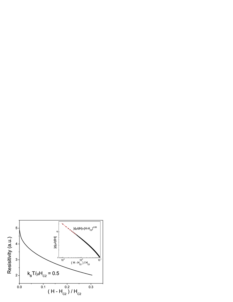
Figure 2: (Color online) Field dependence of the electron-magnon resistivity for a fixed temperature in region II of the phase diagram of Fig.1. The inset shows the field dependence of the modulus of the derivative $d\rho/dH$, which diverges as a power law when $H$ approaches $H_{C2}$.

The thermodynamic properties of the system close to $H_{C2}$ can be easily obtained in the soft mode scenario. They are essentially those of a system of non-interacting bosons. The temperature and field dependent contribution of the spin-wave excitations to the specific heat $C_{V}$ can be shown to have a form similar to that of the electrical resistivity. We get, $C_{V}\propto$ $I_{F}(H,T)$, with $I_{F}(H,T)$ given in Eq.6. Consequently, in region II, which includes the line $H=H_{C2\text{,}}$, the specific heat has a simple power law dependence, $C_{V}\propto(k_{B}T/\mu H_{C2})^{3/2}$. In region I, the field and temperature dependence of $C_{V}$ is the same as that of the resistivity given in Eq. 7. The magnetization at the critical field $H_{C2}$ decreases with a $T^{3/2}$ power law. In region I for $H>H_{C2}$ it decreases exponentially due to the gap, $\Delta=\mu(H-H_{C2})$.

IV Two dimensional case

Many heavy fermions systems due to their anisotropy in the crystalline structure have a regime close to their QCP where the critical fluctuations have a two-dimensional character review . For this reason it is interesting to generalize the results obtained above for the case of two dimensions (2d). In $2d$ the relevant integral for the resistivity can be evaluated and we get,

$$\rho_{2d}(h,t)\propto t\,\left(\frac{2h}{t}\coth\frac{h}{2t}-4\ln 2-4\ln\sinh\frac{h}{2\,t}\right)$$ (8)

where $h=(H-H_{C2})/H_{C2}$ and $t=k_{B}T/\mu H_{C2}$. In the limit $(h/t)\rightarrow 0$, this reduces to

$$\rho_{2d}(h,t)=\rho_{2d}^{0}(1+\ln\frac{t}{h})t$$ (9)

This resistivity varies nearly linear in temperature (Fig.3) but for $H\rightarrow H_{C2}$ ($h\rightarrow 0$) it is not defined for finite temperatures. This is related to the fact that for an isotropic system there is no long range order in two dimensions at any finite temperature due to the creation of an infinite number of magnons. The systems we are considering are in fact three dimensional, although they may exhibit in some region of their phase diagram a $2d$ behavior. However, this is just a regime which will cross over to $3d$ sufficiently close to the transition. Consequently this divergence of $\rho_{2d}(0,t)$ should not interfere with the actual observation of a nearly linear temperature dependence of the resistivity of real systems in some range of region II. In $2d$ the spin-wave contribution to the specific heat, as before, has a similar field and temperature dependence of the resistivity due to electron-magnon scattering. We find in this case ($(h/t)\rightarrow 0$) that in region II (Fig.3),

$$\frac{C_{V}(h,t)}{T}\propto a(1+\ln\frac{t}{h}).$$

The decrease of the magnetization with temperature in a fixed field in this region also has a field and temperature dependence similar to Eq. 9.

Figure 3: Semi-logarithmic plot of the resistivity $\rho$ and specific heat $C_{V}$ divided by T in 2d. Inset shows $\rho$ and $C_{V}$ versus T.

Finally, in region I the specific heat, magnetization and resistivity have an exponential term, as in Eq. 7. Only the temperature dependence of the pre-factor is dependent on dimensionality. This makes it difficult to distinguish a $2d$ from a $3d$ regime in this region, either in thermodynamic or transport measurements.

V Conclusions

We have obtained the electrical and thermodynamic properties of a metallic antiferromagnetic system due to spin-wave modes close to a zero temperature field induced transition. The existence of these excitations close to this phase transition is a general phenomenon, depending only on the appearance of a symmetry-broken state below $H_{C2}$. The resistivity is determined by the scattering of quasi-particles by ferromagnetic-like magnons which become gapless at the transition. The contribution of the spin-wave modes to the thermodynamic and transport properties is distinct in different regions of the phase diagram. In region I, this is exponentially suppressed by the gap $\Delta=\mu(H-H_{C2})$, but in region II these modes are effectively gapless and give rise to important contributions. Notice that these contributions should be considered in addition to those of other quasi-particles. For example, in region I, it has been observed fieldinduced a significant $T^{2}$ term in the resistivity probably due to electron-electron interaction. This temperature dependence of the resistivity is different from that arising from spin-wave scattering which in turn is exponentially suppressed by the gap. In region II however, the spin-wave term is large and its power law temperature dependence is similar to that associated with non-Fermi liquid behavior close to a QCP 11 . This will make it difficult to separate this contribution from that of other quasi-particles. The interaction of the latter with the spin-wave modes may even give rise to substantial mass renormalization. The same remarks apply for the thermodynamic properties in both regions.

The temperature dependence of the thermodynamic properties at the critical field $H_{C2}(T=0)$ is similar to that predicted by the scaling theory of a QCP with a dynamic exponent $z=2$ 11 . In the present case, this value of $z$ reflects the ferromagnetic-like dispersion of the magnons and not the antiferromagnetic nature of the transition. In the extreme metamagnetic case of an Ising antiferromagnet in an external longitudinal field, a renormalization group approach yields a phase diagram where the $T=0$ transition at $H_{C2}$ is not associated with a fixed point. The point ($H=H_{C2},T=0$) is just an ordinary point that flows to ($H=0,T=T_{N}$) as any point in the line of second order transitions $H=H_{C2}(T)$, since the magnetic field turns out to be an irrelevant parameter raimundo . Notice that the spin-wave approach presented above is independent whether the $T=0$ transition at $H_{C2}$ is associated or not with a fixed point.

- (1) For a review see G. Stewart, Rev. Mod. Phys. 73, 797 (2001).
- (2) M. A. Continentino, G. Japiassu and A. Troper, Phys. Rev. B 39, 9734, (1989); A. J. Millis. Phys. Rev. B 48, 7183 (1993); T. Moriya and T. Takimoto, J. Phys. Soc Jap. 64 960 (1995).
- (3) M. A. Continentino, S. N. de Medeiros, M. T. D. Orlando, M. B. Fontes and E. M. Baggio-Saitovitch, Phys. Rev. B 64, 012404 (2001).
- (4) J. Custers, et al., Nature 423, 524 (2003); J. Paglione et al. Phys. Rev. Lett. 91, 246405 (2003). A. McCollam, et al. Physica B359, 1 (2005); F. Ronning, C. Capan, A. Bianchi, R. Movshovich, A. Lacerda, M. F. Hundley, J. D. Thompson, P. G. Pagliuso, and J. L. Sarrao, Phys. Rev. B 71, 104528 (2005); S. L. Bud’ko, E. Morosan, and P. C. Canfield Phys. Rev. B 69, 014415 (2004); Y. Tokiwa, A. Pikul, P. Gegenwart, F. Steglich, S.L. Bud’ko, P.C. Canfield, cond-mat/0511125; E. Morosan, S. L. Bud’ko, Y. A. Mozharivskyj, P. C. Canfield, cond-mat/0506425; P. G. Niklowitz, G. Knebel, J. Flouquet, S. L. Bud’ko, P. C. Canfield, cond-mat/0507211.
- (5) F. Keffer in Encyclopedia of Physics, Vol. XVIII/2, edited by S. Flügge, Springer-Verlag, p.1 (1966).
- (6) H. Yamada and S. Takada, Prog. of Theor. Phys., 49, 1401 (1973).
- (7) A. Demuer, et al., J. Phys. Condens. Matter 13, (2001), 9335.
- (8) W. Knafo, S. Raymond, B. Fak , et al., J. Phys.-Cond. Mat. 15, 3741 (2003).
- (9) F. B. Anderson and H. B. Callen, Phys. Rev. 136, A1068 (1964).
- (10) M. A. Continentino, Quantum Scaling in Many-Body Systems, World Scientific, Singapore, Lecture Notes in Physics - vol. 67 (2001).
- (11) S. L. A. de Queiroz and R. R. dos Santos, J. Phys. C: Solid State Phys. 21, 1995 (1988).