Collective excitations in unconventional charge-density wave systems

Abstract

The excitation spectrum of the $t$-$J$ model is studied on a square lattice in the large $N$ limit in a doping range where a $d$-$density$-$wave$ (DDW) forms below a transition temperature $T^{\star}$. Characteristic features of the DDW ground state are circulating currents which fluctuate above and condense into a staggered flux state below $T^{\star}$ and density fluctuations where the electron and the hole are localized at different sites. General expressions for the density response are given both above and below $T^{\star}$ and applied to Raman, X-ray, and neutron scattering. Numerical results show that the density response is mainly collective in nature consisting of broad, dispersive structures which transform into well-defined peaks mainly at small momentum transfers. One way to detect these excitations is by inelastic neutron scattering at small momentum transfers where the cross section (typically a few per cents of that for spin scattering) is substantially enhanced, exhibits a strong dependence on the direction of the transferred momentum and a well-pronounced peak somewhat below twice the DDW gap. Scattering from the DDW-induced Bragg peak is found to be weaker by two orders of magnitude compared with the momentum-integrated inelastic part.

I Introduction

The electron density operator $\rho$ on a lattice has in momentum space the general form,

$$\rho({\bf q})={1\over N_{c}}\sum_{{\bf k}\sigma}\gamma({\bf k},{\bf q})c^{\dagger}_{\sigma}({\bf k+q})c_{\sigma}(\bf k).$$ (1)

$c^{\dagger}_{\sigma}({\bf k}),c_{\sigma}(\bf{k})$ are electron creation and annihilation operators with momentum $\bf k$ and spin projection $\sigma$, $N_{c}$ is the number of primitive cells, $\bf q$ the transferred momentum, and $\bf k$ characterizes the relative motion of electron and hole. If both particles reside always on the same lattice site $\gamma$ is independent on $\bf k$ and $\rho$ describes a usual density wave. This wave may condense for some wave vector $\bf q$ different from the reciprocal lattice vectors of the unmodulated lattice and a conventional charge density wave (CDW) state is obtained. If the electron and hole explore different sites $\gamma$ depends on $\bf k$ and the condensation of this wave yields a CDW state with an internal symmetry described by the ${\bf k}$ dependence of $\gamma$. We will call this state in the following an unconventional CDW stateMaki1 . Proposals for systems with an unconventional CDW state include organic conductorsMaki1 ; Maki2 and the pseudogap phase of high-temperature superconductorsHsu ; Cappelluti ; Benfatto ; Chakravarty .

Static and fluctuating density waves of the general form of Eq.(1) can be observed by various experimental probes. The vector potential generated by the magnetic moment of neutrons influences the hopping elements of electrons via the Peierls substitution. Thus neutrons probe orbital magnetic fluctuations associated with density fluctuations. As shown in Ref.Hsu, the resulting neutron cross section is related to the imaginary part of a retarded density-density correlation function, where $\gamma$ is given by,

$$\gamma({\bf k},{\bf q}) = {{8i\pi e\mu_{0}t_{eff}}\over{\hbar c|{\bf q}|}}\times$$

$$\Bigl{(}\sum_{j=x,y}{\alpha_{j}\over q_{j}} ( (1-\cos{q_{j}})\cos{k_{j}}+\sin{q_{j}}\sin{k_{j}})\Bigr{)},$$ (2)

with

$${\alpha}={\mu\over{\mbox{\unboldmath$\mu_{0}$}}}\times{q\over|q|}\mbox{\unboldmath$.$}$$ (3)

The expression Eq.(2) applies to a solid of square layers with lattice constant $a$ which we put, together with $\hbar$ to one in the following. $t_{eff}$ is an effective nearest neighbor hopping integral, $c$ the velocity of light, ${\mu}$ the magnetic moment of the neutrons, and $\mu_{0}=\sqrt{{{\mbox{\boldmath$\mu$}\unboldmath^{2}}\over 3}}$. We neglect hopping between the layers as well as a small contribution to $\gamma$ from second-nearest neighbor hoppings $\sim t^{\prime}$. Similarly, inelastic light and non-resonant X-ray scattering are determined by the Raman or the X-ray scattering amplitude which corresponds to the following expression for $\gamma$Devereaux ,

$$\gamma({\bf k},{\bf q})=\sum_{\alpha\beta}e^{s}_{\alpha}{{\partial^{2}\epsilon({\bf k}+{\bf q}/2)}\over{\partial k_{\alpha}\partial k_{\beta}}}e^{i}_{\beta}.$$ (4)

${\bf e}^{i}$ and ${\bf e}^{s}$ are the polarization vectors of the incident and scattered light, respectively, and $\epsilon({\bf k})$ the one-particle energy. In contrast to Refs.Hsu, ; Devereaux, we assumed that the Peierls substitution is made in the renormalized Hamiltonian so that the renormalized hopping $t_{eff}$ and one-electron band appear in Eqs.(2) and (4). For Raman scattering the momentum transfer is practically zero whereas no such restriction exists for X-ray scattering.

Microscopic models for interacting electrons usually contain interactions between local charge densities or spin densities, such as, the Coulomb or Heisenberg interaction. $\bf k$-dependent densities of the form of Eq.(1) become important if the exchange terms are competing or dominating the direct, Hartree-like terms. The excitonic insulator is such a case where the Coulombic exchange terms not only create excitons but force them to condense into a new ground stateRice . These ideas were applied to high-T_c cuprates by EfetovEfetov assuming that the barely screened Coulomb interaction between layers produces interlayer excitons and their condensation. More recently, it was recognized that the $t$-$J$ model in the large $N$ limit ($N$ is the number of spin components) shows a transition to a charge-density wave state with internal $d$-wave symmetry (DDW) at low dopingCappelluti with a transition temperature $T^{\star}$. This model describes electrons in the $CuO_{2}$ planes of high-T_c cuprates and identifies the pseudogap phase at low dopings with a DDW state. One may expect that near the phase boundary to the DDW state or in the DDW state density fluctuations of the form of Eq.(1) become important and, according to the above discussion, could be detected by neutron or X-ray scattering. It is therefore the purpose of this paper to calculate the general density response of this model, both above and below $T^{\star}$, and to make predictions for the magnitude and the momentum and polarization dependence of neutron and X-ray cross sections.

The order parameter of a commensurate DDW state with wave vector $(\pi,\pi)$ is purely imaginary which follows from the hermiticity of the large $N$ Hamiltonian. As a consequence, circulating, local currents accompagny in general density fluctuations in the DDW state producing orbital magnetic moments localized on the plaquettes of the square lattice. The circulating currents fluctuate above and freeze into a staggered flux phase below $T^{\star}$. Most previous calculations considered ${\bf q}=0$ quantities such as the frequency-dependent conductivityBenfatto1 ; Aristov ; Benfatto2 ; Carbotte or Raman scatteringZeyher4 ; Carbotte . Calculations for finite momentum transfersTewari to be presented below are interesting because they probe the local properties of the density fluctuations and the flux lattice.

In section II we will first reformulate the large $N$ limit of the $t$-$J$ model in terms of an effective Hamiltonian which contains usual electron creation and annihilation operators (i.e., no constraint operators), renormalized bands and an interaction between several charge density waves. This effective model contains as a special case the models used in Refs.Maki1, ; Carbotte, in discussing anomalous charge density waves. We then extend previous normal-state calculations of the density response, given by a 6x6 susceptibility matrix $\chi$, to the DDW state using the Nambu formalism. The obtained expressions hold for all momenta $\bf q$ and are general enough to discuss the dispersion of collective modes and the momentum and polarization dependencies of experimental cross sections.

Section III contains numerical results for the formulas presented in section II. In subsection A the density fluctuation spectrum in the d-wave channel will be discussed as a function of momentum, both above and below $T^{\ast}$. In subsections B and C results for the cross sections for non-resonant inelastic X-ray scattering and for polarized and unpolarized neutron scattering will be given, and subsection D compares the magnitude of $\bf q$ integrated neutron cross sections for spin and for orbital scattering. Section IV contains our conclusions.

II Density response in the d-CDW state

In Refs.Zeyher1, ; Zeyher2, it has been shown that the density response in the normal state of the $t$-$J$ model at large $N$ can be obtained by using the following two sets of density operators,

$$\rho^{\prime}_{\alpha}({\bf q})={1\over N_{c}}\sum_{{\bf k}\sigma}E_{\alpha}({\bf k},{\bf q})c^{\dagger}_{\sigma}({\bf k}+{\bf q})c_{\sigma}({\bf k}),$$ (5)

$$\rho_{\beta}({\bf q})={1\over N_{c}}\sum_{{\bf k}\sigma}F_{\beta}({\bf k})c^{\dagger}_{\sigma}({\bf k}+{\bf q})c_{\sigma}({\bf k}),$$ (6)

with

$$E_{\alpha}({\bf k},{\bf q})=(1,t({\bf k}+{\bf q})+J({\bf q}),\gamma_{3}({\bf k}),\gamma_{4}({\bf k}),\gamma_{5}({\bf k}),\gamma_{6}({\bf k})),$$ (7)

and

$$F_{\beta}({\bf k})=(t({\bf k}),1,2J\gamma_{3}({\bf k}),2J\gamma_{4}({\bf k}),2J\gamma_{5}({\bf k}),2J\gamma_{6}({\bf k})).$$ (8)

Compared to Refs.Zeyher1, ; Zeyher2, a slight change in the representation of the basis functions has been made by using the symmetrized functions

$$\gamma_{3,5} = (\cos{k_{x}}\pm\cos{k_{y}})/2,$$

$$\gamma_{4,6} = (\sin{k_{x}}\pm\sin{k_{y}})/2,$$ (9)

where the subscripts 3 and 4 refer to the $+$ and 5 and 6 to the $-$ sign. Here, and in the following, we put the lattice constant of the square lattice to $1$. $t({\bf k})$ and $J({\bf k})$ are the Fourier transforms of the hopping amplitudes $t_{ij}$ and the Heisenberg term $J_{ij}$, respectively. Including nearest and second nearest neighbor hoppings $t$ and $t^{\prime}$, respectively, we have

$$t({\bf k})=2t(\cos{k_{x}}+\cos{k_{y}})+4t^{\prime}\cos{k_{x}}\cos{k_{y}}.$$ (10)

The corresponding density-density Matsubara Green’s function matrix is defined by

$$\chi_{\alpha\beta}({\bf q},i\omega_{n})=-\int_{0}^{1/T}d\tau e^{-i\omega_{n}\tau}<T_{\tau}\rho^{\prime}_{\alpha}({\bf q}\tau)\rho^{\dagger}_{\beta}({\bf q}0)>.$$ (11)

The general solution for $\chi$ in the normal state has been given in the large $N$ limit and the dispersion of macroscopic density fluctuations, determined by the element $\chi_{12}$, have been discussedGehlhoff ; Zeyher1 . At lower temperatures and dopings the density component $E_{5}({\bf k},{\bf Q})$ freezes in for a wave vector $\bf Q$ approximately equal to $(\pi,\pi)$, leading to the DDW state.

The Hilbert space of the $t$-$J$ model does not contain double occupancies of sites, its operators are therefore $X$ and not the usual creation and annihilation operators $c^{\dagger}_{i\sigma}$ and $c_{i\sigma}$ of second quantization. In the large $N$ limit the $t$-$J$ model becomes, however, equivalent to the following effective Hamiltonian in terms of usual creation and annihilation operators,

$$H_{eff}=\sum_{{\bf k}\sigma}\epsilon({\bf k})c^{\dagger}_{\sigma}({\bf k})c_{\sigma}({\bf k})-{N_{c}\over 2}\sum_{\alpha=1}^{6}\sum_{\bf q}\rho_{\alpha}^{\prime}({\bf q})\rho_{\alpha}^{\dagger}({\bf q}).$$ (12)

$\epsilon({\bf k})$ are the one-particle energies in the large $N$ limit,

$$\epsilon({\bf k})={\delta\over 2}t({\bf k})-{J({\bf k})\over 2}\cdot{1\over N_{c}}\sum_{\bf p}\cos(p_{x})f(\epsilon({\bf p})-\mu).$$ (13)

$\mu$ is the renormalized chemical potential and $f$ the Fermi function. The second term in Eq.(12) represents an effective interaction originating from the functional derivative of the self-energy with respect to the Green’s function. This interaction is hermitean though its present form does not show this property explicitly because of the chosen compact form to represent it. Using Eqs.(5) and (6) one easily verifies that the sum of the terms $\alpha=3...6$ represent the Heisenberg interaction, written as a charge- charge interaction and as a sum of four separable kernels. The terms $\alpha=1,2$ originate from the constraint which acts in $H_{eff}$ as a two-particle interaction. $H_{eff}$ and the original $t$-$J$ Hamiltonian in the large $N$ limit become equivalent if only bubble diagrams generated by the second term in $H_{eff}$ and no self-energy corrections are taken into account. In the DDW state $<\rho_{\alpha}({\bf Q})>$ and $<\rho^{\prime}_{\alpha}({\bf Q})>$ become non-zero for $\alpha=5$. We rewrite $H_{eff}$ as,

$$H_{eff} = \sum_{{\bf k}\sigma}\epsilon({\bf k})c^{\dagger}_{\sigma}({\bf k})c_{\sigma}({\bf k})-N_{c}<\rho^{\prime}_{5}({\bf Q})>\rho^{\dagger}_{5}({\bf Q})$$ (14)

$$- {N_{c}\over 2}\sum_{\alpha=1}^{6}\sum_{\bf q}\tilde{\rho}_{\alpha}^{\prime}({\bf q})\tilde{\rho}_{\alpha}^{\dagger}({\bf q}).$$

The tilde at the density operators means that only their fluctuating parts should be considered.

In order to be able to use usual diagrammatic rules in the DDW state we introduce the Nambu notation, i.e., the row vector $\psi^{\dagger}_{\sigma}({\bf k})=(c^{\dagger}_{\sigma}({\bf k}),c^{\dagger}_{\sigma}({\bf k}+{\bf Q}))$ and the corresponding column vector obtained by hermitean conjugation. We also make the convention that the momentum in $\psi$ or $\psi^{\dagger}$ are always taken modulo the reduced Brillouin zone (RBZ), i.e., lie in the RBZ. The momentum sums over the (large) Brillouin zone (BZ) are then split into parts inside and outside of the RBZ and the two parts then combined using the Nambu vectors and Pauli matrices. We obtain then,

$$\rho^{\prime}_{\alpha}({\bf q})={1\over N_{c}}{\sum_{{\bf k}\sigma}}^{\prime}\psi^{\dagger}_{\sigma}({\bf k}+{\bf q})\hat{E}_{\alpha}({\bf k},{\bf q})\psi_{\sigma}({\bf k}),$$ (15)

$$\rho_{\beta}({\bf q})={1\over N_{c}}{\sum_{{\bf k}\sigma}}^{\prime}\psi^{\dagger}_{\sigma}({\bf k}+{\bf q})\hat{F}_{\beta}({\bf k})\psi_{\sigma}({\bf k}),$$ (16)

with

$$\hat{F}_{1}({\bf k}) = t^{(1)}({\bf k})P_{o}({\bf k}+{\bf q},{\bf k})+t^{(2)}({\bf k})P_{e}({\bf k}+{\bf q},{\bf k}),$$

$$\hat{F}_{2}({\bf k}) = P_{e}({\bf k}+{\bf q},{\bf k}),$$

$$\hat{F}_{\beta}({\bf q}) = F_{\beta}({\bf k})P_{o}({\bf k}+{\bf q},{\bf k}),$$ (17)

for $\beta=3...6$,

$$\hat{E}_{1}({\bf k},{\bf q}) = \hat{F}_{2}({\bf k}),$$

$$\hat{E}_{2}({\bf k},{\bf q}) = t^{(1)}({\bf k}+{\bf q})P_{o}({\bf k}+{\bf q},{\bf k})$$

$$+ (t^{(2)}({\bf k}+{\bf q})+J({\bf q}))P_{e}({\bf k}+{\bf q},{\bf k}),$$

$$\hat{E}_{\alpha}({\bf k},{\bf q}) = \hat{F}_{\alpha}({\bf k})/2J,$$ (18)

for $\alpha=3...6$, and

$$P_{o}({\bf k}+{\bf q},{\bf k}) = p({\bf k}+{\bf q},{\bf k})\sigma_{3}-i(1-p({\bf k}+{\bf q},{\bf k}))\sigma_{2},$$

$$P_{e}({\bf k}+{\bf q},{\bf k}) = p({\bf k}+{\bf q},{\bf k})\sigma_{0}+(1-p({\bf k}+{\bf q},{\bf k}))\sigma_{1}.$$

$t^{(1)}({\bf k})$ and $t^{(2)}({\bf k})$ are the Fourier transforms of the nearest and second-nearest neighbor hopping amplitudes, $\sigma_{0}$ is the 2x2 unit matrix, and $\sigma_{1},\sigma_{2},\sigma_{3}$ are Pauli matrices. The dash at the summation sign in Eq.(16) means a restriction of the sum to the RBZ. $p({\bf k}+{\bf q},{\bf k})$ with ${\bf k}$ in the RBZ is equal to one if ${\bf k}+{\bf q}$, reduced to the BZ, lies in the RBZ and is zero otherwise. Finally, the first and second terms in $H_{eff}$ can be combined and read in Nambu notation as

$$H^{(0)}_{eff}={\sum_{{\bf k}\sigma}}^{\prime}\psi^{\dagger}_{\sigma}({\bf k})\Big{[}(\epsilon_{+}({\bf k})-\mu)\sigma_{0}$$

$$+\epsilon_{-}({\bf k})\sigma_{3}+\Phi\gamma_{5}({\bf k})\sigma_{2}\Big{]}\psi_{\sigma}({\bf k}).$$ (20)

The energies $\epsilon_{\pm}$ are defined by $(\epsilon({\bf k})\pm\epsilon({\bf k}+{\bf Q}))/2$. $\Phi$ is an abbreviation for the amplitude of the DDW and must be real because of the hermiticity of $H_{eff}$.

Using the above Nambu representation the susceptibility matrix $\chi_{\alpha\beta}$ is obtained by a bubble summation,

$$\chi_{\alpha\beta}(q)=\sum_{\gamma}\chi^{(0)}_{\alpha\gamma}(q)(1+\chi^{(0)}(q))^{-1}_{\gamma\beta}.$$ (21)

Here we used the abbreviation $q=(i\nu_{n},{\bf q})$ with the bosonic Matsubara frequencies $\nu_{n}=2\pi Tn$, where $T$ is the temperature. $\chi^{(0)}(q)$ stands for a single bubble and is given analytically by the expression

$$\chi_{\alpha\beta}^{(0)}(q)={T\over N_{c}}{\sum_{{\bf k}n}}^{\prime}Tr\Big{[}G(k+q)\hat{E}_{\alpha}({\bf k},{\bf q})G(k)\hat{F}^{\dagger}_{\beta}({\bf k})\Big{]},$$ (22)

with the Nambu Green’s function

$$G(k)={{(i\omega_{n}+\mu-\epsilon_{+}({\bf k}))\sigma_{0}+\epsilon_{-}({\bf k})\sigma_{3}+\Phi\gamma_{5}({\bf k})\sigma_{2}}\over{(i\omega_{n}-E_{1}({\bf k}))(i\omega_{n}-E_{2}({\bf k}))}},$$ (23)

and the two eigenenergies

$$E_{1,2}({\bf k})=\epsilon_{+}({\bf k})-\mu\pm\sqrt{\epsilon_{-}^{2}({\bf k})+\gamma_{5}^{2}({\bf k})\Phi^{2}}.$$ (24)

After performing the trace over Pauli matrices and the sum over fermionic Matsubara frequencies in Eq.(22) only the sum over momenta is left for a numerical evaluation. In the normal state we obtain

$$\chi_{\alpha\beta}^{(0)}({\bf q},i\omega_{n})=$$

$${1\over N_{c}}\sum_{\bf k}E_{\alpha}({\bf k},{\bf q})F_{\beta}({\bf k}){{f(\epsilon({\bf k}+{\bf q}))-f(\epsilon({\bf k}))}\over{\epsilon({\bf k}+{\bf q})-\epsilon({\bf k})-i\omega_{n}}}.$$ (25)

Two special cases of Eq.(21) should be mentioned. If $\bf q$ is parallel to the diagonal, i.e., of the form ${\bf q}=(q,q)$, the components 5 and 6 in the matrices, which are odd under reflection at the diagonal, decouple from the other components. At the points ${\bf q}=(0,0)$ and $(\pi,\pi)$ they even decouple from each other so that Eq.(21) can be solved by division, for instanceZeyher3 ,

$$\chi_{55}(q)=\chi_{55}^{(0)}(q)/(1+\chi_{55}^{(0)}(q)),$$ (26)

for ${\bf q}=(0,0)$ and ${\bf q}=(\pi,\pi)$. In the first case $\chi_{55}$ describes the $B_{1g}$ component of Raman scatteringZeyher4 , in the second case amplitude fluctuations of the order parameterTewari . The other special case refers to a DDW without constraintTewari ; Carbotte . Since the components 1 and 2 were caused by the constraint they can be dropped in this case and Eq.(21) reduces to a 4x4 matrix equation. The four components arise because a nearest neighbor charge-charge interaction leads to four separable kernels. If this interaction is furthermore approximated by one kernel, associated with the order parameter, Eq.(21) reduces to one scalar equation, and one arrives at the models of Refs.Maki1, ; Carbotte, .

The above formulas allow to calculate density correlation functions which can be expressed by $\rho^{\prime}$ or $\rho$ defined in Eqs.(5)-(6). The most general case may, however, involve two additional densities $\rho_{0}$ and $\rho^{\prime}_{0}$ in Eqs.(5) and (6), respectively, where $E_{0}$ and $F_{0}$ are general functions of $\bf k$. Going over to the Nambu representation $\hat{E}_{0}$ and $\hat{F}_{0}$ are then linear combinations of the Pauli matrices and general functions of ${\bf k}$. Using the diagramatic rules and the effective Hamiltonian one finds for the general susceptibility $\chi_{00}(q)$,

$$\chi_{00}(q)=\chi_{00}^{(0)}(q)+\sum_{\alpha\beta}\chi^{(0)}_{0\alpha}(q)\chi_{\alpha\beta}(q)\chi^{(0)}_{\beta 0}(q).$$ (27)

$\chi^{(0)}_{00}(q)$ is given by Eq.(22) where both $\alpha$ and $\beta$ have been replaced by $\mathrm{𝟎}$. Similarly, the expressions for $\chi^{(0)}_{0\beta}$ and $\chi^{(0)}_{\alpha 0}$ are obtained from Eq.(22) by replacing only $\alpha$ or $\beta$, respectively, by $\mathrm{𝟎}$. $\chi_{\alpha\beta}$ is given by Eq.(21).

III Numerical results

III.1 D-wave susceptibility $\chi_{55}$

From now on we will write $t=-|t|$ and use $|t|$ as the energy unit. Furthermore, the Heisenberg constant $J$ and the doping $\delta$ will be fixed to the values 0.3 and 0.077, respectively. The mean-field value for the superconducting transition temperature is then practically zero so that we deal with a pure DDW system. Fig.1 shows the negative imaginary part of the retarded susceptibility $\chi_{55}({\bf q},\omega)$, denoted by $\chi^{\prime\prime}_{55}$ in the following, as a function of $\omega$ in the normal state, using $t^{\prime}=-0.3$ and a small imaginary part $\eta=0.001$. We have chosen the component $\chi_{55}$ and the wave vector ${\bf q}=(\pi,\pi)$ because the transition

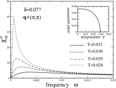
Figure 1: Negative imaginary part of $\chi_{55}$ of the $t$-$J$ model at large $N$ for $t^{\prime}=-0.3$, $\eta=0.001$, ${\bf q}=(\pi,\pi)$, and doping $\delta=0.077$. Inset: $DDW$ order parameter $\Phi$ as a function of temperature $T$.

to the DDW state occurs in this symmetry channel and near this wave vector. Decreasing the temperature from $T=0.032$ to $T=0.028$ shifts spectral weight in the overdamped spectrum from large to small frequencies until a sharp and intense peak appears very near to the transition point

Figure 2: $\chi_{55}^{\prime\prime}$ in the normal state at $T=0.039$ calculated for $t^{\prime}=-0.3$, $\delta=0.077$, and along the line $\Gamma$-$S$-$X$-$\Gamma$ in the Brillouin zone.

$T^{\star}\sim 0.028$. Decreasing further the temperature the spectrum becomes again broad and moves to higher frequencies. The inset of Fig.1 shows the temperature dependence of the DDW order parameter $\Phi$ which exhibits the usual mean-field behavior.

Fig.2 shows a three-dimensional plot of $\chi^{\prime\prime}_{55}$ as a function of $\omega$ in the normal state at $T=0.039$. The momentum runs from the point $\Gamma=(0,0)$ to the points $S=(\pi,\pi)$ and $X=(0,\pi)$, and back to the point $\Gamma$. The curves for $\Gamma$, $S$ and $X$ are drawn as thick lines to facilitate the visiualization. According to Eq.(25), and similar as in the case of the usual charge susceptibility, $\chi_{55}$ exhibits a singular behavior at small frequencies and wave vectors in the limit $\eta\rightarrow 0$: Fixing the momentum to ${\bf q}=(0,0)$ $\chi_{55}(0,\omega)$ is zero for any finite frequency $\omega$. Putting $\omega$ to zero and taking the limit ${\bf q}\rightarrow 0$ $\chi_{55}$ approaches a finite value. This explains the absence of a thick line at $\Gamma$ in Fig.2. Moving the momentum from $\Gamma$ to $S$ the zero-frequency peak of measure zero at $\Gamma$ aquires a finite width, i.e., a finite spectral weight, and at the same time peaks at a finite frequency. Both the width and the peak increase first rapidly with momentum. The peak position passes then through a maximum at $\omega\sim 0.04$, starts to decrease, and reaches a minimum at $S$ signalling the transition to the DDW state at lower temperatures. The width of the peak as well as the extension and intensity of the slowly decaying structureless background increases up to the point $S$. Moving along the direction $S$-$X$-$\Gamma$ the low-frequency peak looses rapidly spectral weight, vanishes practically at $X$, and recovers somewhat towards $\Gamma$. At the same time a well-pronounced, strong high-frequency peak develops, its frequency decreases monotonically along the above path, and its intensity shows a maximum near the point $X$. The dispersion of this high-frequency peak is $\sim\sin{k_{x}}$ between $\Gamma$ and $X$, i.e., it is identical with the sound wave due to usual density fluctuationsGehlhoff . This means that d-wave density fluctuations, described by $\chi_{55}^{\prime\prime}$, strongly couple to usual density fluctuations along the path $S$-$X$-$\Gamma$ whereas such a coupling is forbidden by symmetry along $\Gamma$-$S$.

Figure 3: $\chi_{55}^{\prime\prime}$ at T=0. calculated for $t^{\prime}=-0.3$, $\delta=0.077$, and along the lines $\Gamma$-$S$-$X$-$\Gamma$ in the Brillouin zone.

Fig.3 shows the same 3d plot as Fig.2 but the calculation is now performed at T=0 in the DDW state. Differences in the two figures thus have to be ascribed to the formation of the DDW. Taking the different scales in the two figures into account one sees that the intensity of the high-frequency peak due to usual density fluctuations did not change much. Big changes, however, occur at low frequencies. $\chi_{55}^{\prime\prime}$ no longer vanishes at finite frequencies at the $\Gamma$-point but rather shows there a well-pronounced and strong peak. Moving away from the $\Gamma$ point this peak looses rapidly intensity whereas its frequency does not change much.

To understand the origin and the properties of the low-frequency peak in more detail we have plotted in Fig.4 $\chi_{55}^{\prime\prime}$ and ${\chi_{55}^{(0)}}^{\prime\prime}$ as a function of frequency for several $\bf q$ values between the $\Gamma$ and $S$ point. The dashed line in the upper diagram represents ${\chi_{55}^{(0)}}^{\prime\prime}$ at the wave vector ${\bf q}=(\pi,\pi)$. It contains only interband transitions across the DDW gap, mainly between the points $X$ and $Y$ and between the hot spots on the boundaries of the RBZ. The intraband contribution is zero by symmetry at $S$. Since $\Phi$ is about 0.07 the interband transitions lead to a broad peak somewhat higher than twice the DDW gap. The solid curve in the upper diagram of Fig.4 represents $\chi_{55}^{\prime\prime}$ at $S$. It shows a much more pronounced peak than the dashed curve which originates from the denominator in Eq.(26), i.e., which represents a collective excitation. It corresponds to the amplitude mode of the DDW, where the order parameter $\Phi$ is modulated without changing its d-wave symmetry. Its frequency is somewhat smaller than $2\Phi$ which is expected for a d-wave state. For an isotropic s-wave ground state the two frequencies would be exactly the same.

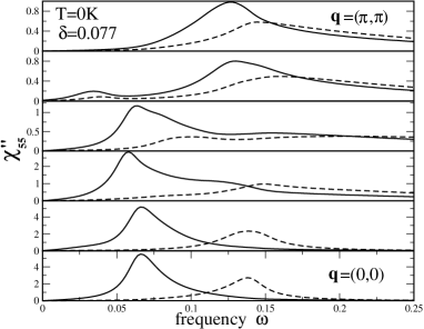
Figure 4: $\chi_{55}^{\prime\prime}$ (solid lines) and $\chi_{55}^{(0)^{\prime\prime}}$ (dashed lines) for momenta along the diagonal ${\bf q}=(q,q)$.

The lowest panel in Fig.4 shows the same susceptibilities at the $\Gamma$ point. ${\chi_{55}^{(0)}}^{\prime\prime}$ again contains no intraband but only interband contributions consisting of vertical transitions which probe directly the DDW gap. As a result, ${\chi_{55}^{(0)}}^{\prime\prime}$ exhibits a well-defined peak at $2\Phi$ and a long-tail towards smaller frequencies due to the momentum dependence of the order parameter. The solid curve, representing $\chi_{55}^{\prime\prime}$, exhibits a well-pronounced peak much below $2\Phi$. It corresponds to a bound state inside the d-wave gap created by multiple scattering of the excitations across the gap due to the Heisenberg interaction. Due to its large binding energy the density of states inside the gap is rather small at the peak position so that the width of the peak is substantialy smaller than that of the amplitude mode at the momentum $(\pi,\pi)$. PreviouslyZeyher4 , we have associated this peak with the $B_{1g}$ peak seen in Raman scattering in high-T_c superconductors. Note that there is roughly a factor 5 difference in the scales of the top and bottom panels in Fig.4. It means that the amplitude mode of the DDW order parameter has a much larger spectral weight and also smaller width at the $\Gamma$ than at the $S$ point.

For momenta $\bf q$ between $\Gamma$ and $S$ both intra- and interband transitions contribute to ${\chi_{55}^{(0)}}^{\prime\prime}$. The intraband part, reflecting the residual Fermi arcs in the DDW state, turns out to be in general substantially smaller than the interband part and consists of a broad peak which disperses roughly as $\sin(q)$ and which looses its intensity when approaching $\Gamma$ or $S$. So only the low-frequency tails and the structure around the frequency 0.04 in the second panel from above can be attributed to intraband scattering, the remaining spectral weight is due to interband scattering. Going from $\Gamma$ to $S$ the solid lines show the dispersion of the amplitude mode which is in general well below the main spectral peak in ${\chi_{55}^{(0)}}^{\prime\prime}$, representing a resonance mode with a frequency and width determined mainly by the denominator in Eq.(26). From the different scales used in each panel it is evident that the intensity of the amplitude mode strongly decays away from the $\Gamma$ point in agreement with Fig.3.

III.2 Non-resonant inelastic X-ray scattering

Specifying the polarization vectors of the incident and scattered light and using Eqs.(13) and (10) for the electron dispersion the cross section for inelastic X-ray scattering is determined by $\chi_{X}^{\prime\prime}$ and $\chi_{X}$ is obtained as a linear combination of the susceptibility matrix elements $\chi_{\alpha\beta}$. As an example, consider the case ${\bf e}^{i}=(1,1)/\sqrt{2},{\bf e}^{s}=(1,-1)/\sqrt{2}$, which yields for ${\bf q}=0$ the $B_{1g}$ component of Raman scattering. Choosing the symmetry direction ${\bf q}=(q,q)$, we find,

$$\chi_{X}({\bf q},i\omega_{n})={2t_{eff}^{2}\over{J}}\Bigl{(}\cos{{}^{2}}({{q}\over 2})\chi_{55}({\bf q},i\omega_{n})$$

$$+\sin{{}^{2}}({q\over 2})\chi_{66}({\bf q},i\omega_{n})-\sin(q)\chi_{56}({\bf q},i\omega_{n})\Bigr{)},$$ (28)

Figure 5: D-wave cross section for nonresonant, inelastic $X$-ray scattering for the $t$-$J$ model at large $N$ in the DDW state at $T=0$. The momentum varies along the points $\Gamma$-$S$-$X$-$\Gamma$ in the Brillouin zone.

with the effective nearest-neighbor hopping element $t_{eff}$ determined by the large $N$ dispersion of Eq.(13). The second-nearest hopping element $t^{\prime}$ drops out in the considered symmetry. In Fig.5 we have plotted $\chi_{X}$ without this prefactor along the points $\Gamma$-$S$-$X$-$\Gamma$ generalizing Eq.(28) to an arbitrary ${\bf k}$ point in the Brillouin zone. One feature of $\chi_{X}^{\prime\prime}$ is that the high-frequency side bands due to usual density fluctuations are practically absent. This may be explained by the fact that the various contributions to $\chi_{X}^{\prime\prime}$ have both signs causing large cancellation effects. Another difference between Figs.3 and 5 occurs around the point $S$ where additional structure is seen in $\chi_{X}^{\prime\prime}$ due to the component $\chi_{66}$.

III.3 Inelastic neutron scattering

Using the symmetry-adapted functions Eq.(9) the expression for $\gamma$, Eq.(2), can be written as,

$$\gamma({\bf k},{\bf q})={{8\pi ie\mu_{0}t_{eff}}\over{\hbar c|{\bf q}|}}\sum_{\beta=3}^{6}B_{\beta}({\bf q})\gamma_{\beta}({\bf k}),$$ (29)

with

$$B_{3,5}={\alpha_{x}\over q_{x}}(1-cosq_{x})\pm{\alpha_{y}\over q_{y}}(1-cosq_{y}),$$ (30)

$$B_{4,6}={\alpha_{x}\over q_{x}}sinq_{x}\pm{\alpha_{y}\over q_{y}}sinq_{y},$$ (31)

where the subscripts $3,4$ refer to the $+$ and $5,6$ to the $-$ signs, respectively. The charge correlation function, describing neutron scattering, is given by,

$$\chi_{N}({\bf q},\omega)={1\over{2J}}\Bigl{(}{{8\pi e\mu_{0}t_{eff}}\over{c|{\bf q}|}}\Bigr{)}^{2}\sum_{\beta,\delta}B_{\beta}({\bf q})B_{\delta}({\bf q})\chi_{\beta\delta}({\bf q},\omega).$$ (32)

Figure 6: $\chi_{N}^{\prime\prime}$ describing neutron scattering as a function of $\omega$ along the line $\Gamma$-$S$-$X$-$\Gamma$ in the Brillouin zone in the DDW state at $T=0$ using $t^{\prime}=-0.3$, $\delta=0.077$, $q_{z}=0.5$, and $\eta=0.05$.

Fig. 6 shows $\chi_{N}^{\prime\prime}({\bf q},\omega)$ as a function of $\omega$ for momenta along the symmetry line $\Gamma$-S-X-$\Gamma$ in the Brillouin zone for the fixed momentuma transfer $q_{z}=0.5$. The spin of the neutrons was assumed to be polarized along the $z$-axis. The spectra show essentially one more or less well-defined peak which disperses roughly between the frequencies $0.1-0.2$. Similarly as in Fig.4 this peak describes a mainly collective excitation of the system related to a bound state inside the DDW gap. In spite of the rather large momentum transfer $q_{z}=0.5$ the peak intensity increases substantially towards the point $\Gamma$. This increase becomes more and more pronounced if $q_{z}$ is further lowered until it diverges like $1/|{\bf q}|^{2}$ in the limit $q_{z}\rightarrow 0$.

An important special case of Eq.(32) is scattering by unpolarized neutrons. Averaging over all spin directions for the neutrons yields the charge correlation function $\chi_{N,u}$ for scattering with unpolarized neutrons,

$$\chi_{N,u}({\bf q},\omega)=\sum_{\alpha\beta}F_{\alpha\beta}({\bf q})\chi_{\alpha\beta}({\bf q},\omega),$$ (33)

with

$$F_{\alpha\beta}={1\over{2J}}\Bigl{(}{{8\pi e\mu_{0}t_{eff}}\over{c|{\bf q}|}}\Bigr{)}^{2}<B_{\alpha}({\bf q})B_{\beta}({\bf q})>_{av},$$ (34)

where $<...>_{av}$ denotes an average over all directions of the moment of the neutron. We obtain,

$$<B_{\alpha}({\bf q})B_{\beta}({\bf q})>_{av}={1\over{|{\bf q}|^{2}}}[(q_{y}^{2}+q_{z}^{2})f_{\alpha}f_{\beta}$$

$$-q_{x}q_{y}(f_{\alpha}g_{\beta}+g_{\alpha}f_{\beta})+(q_{x}^{2}+q_{z}^{2})g_{\alpha}g_{\beta}],$$ (35)

with $f_{3}=f_{5}=(1-\cos{q_{x}})/q_{x}$, $g_{3}=-g_{5}=(1-\cos{q_{y}})/q_{y}$, $f_{4}=f_{6}=\sin{q_{x}}/q_{x}$, $g_{4}=-g_{6}=\sin{q_{y}}/q_{y}$. $\chi_{N,u}({\bf q},\omega)$ diverges at small momentum transfers in the DDW state. To extract its singular part one may take the limit ${\bf q}\rightarrow 0$ in the $f$, $g$, and $\chi$ functions. One obtains then,

$$\chi_{N,u}\sim({1\over{|{\bf q}|^{2}}}+{q_{z}^{2}\over{|{\bf q}|^{4}}})\chi_{66}(0,i\omega_{n}).$$ (36)

In the normal state $\chi_{66}$ vanishes at ${\bf q}=0$ for any finite frequency as can be seen from the explicit expression Eq.(25). In contrast to that it is finite at ${\bf q}=0$ in the DDW state describing a continuum of particle-hole excitations with zero total momentum across the gap. As a result $\chi_{N,u}$ diverges quadratically in the momentum ${\bf q}_{\|}$ parallel to the layers for $q_{z}=0$. This divergence is caused by the long-range part of the interaction between the magnetic moment of the neutron and the electrons in the layers. It is thus a real effect causing a singular forward scattering contribution in the cross section. Integrating $\chi_{N,u}^{\prime\prime}$ over ${\bf q}$ diverges logarithmically in a strictly 2d description at $q_{z}=0$ whereas it remains finite in three dimensions.

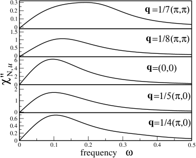
Figure 7: $\chi_{N,u}^{\prime\prime}$ describing scattering with unpolarized neutrons as a function of $\omega$ for momenta around the point $\Gamma$ in the DDW state at $T=0$ using $t^{\prime}=-0.3$, $\delta=0.077$ and $q_{z}=0.5$.

The large enhancement of $\chi_{N,u}^{\prime\prime}$ near the point $\Gamma$ is illustrated in Fig.7. The curve at $\Gamma$ shows a peak at $\omega\sim 0.1$ well inside the gap of $2\Delta_{0}\sim 0.14$, which disperses to higher frequencies moving away from $\Gamma$, especially, along the diagonal. More dramatic is, however, the rapid decay of the intensity of the peak away from $\Gamma$ which can be seen from the different scales used in plotting the various panels.

Another special case of Eq.(32) is obtained for an arbitrary polarization for the neutron moment and a vanishing momentum transfer in the $z$ direction, i.e., for ${\bf q}=(q_{x},q_{y},0)$. The functions $B_{i}$ assume in this case the form for $i=3,4$,

$$B_{i}={\mu_{z}\over{\mu_{0}|{\bf q}|}}(-q_{y}f_{i}+q_{x}g_{i}),$$

$$B_{i+2}={\mu_{z}\over{\mu_{0}|{\bf q}|}}(-q_{y}f_{i}-q_{x}g_{i}).$$ (37)

The polarization dependence of $\chi_{N}$ is simply $\cos{{}^{2}}\theta$ where $\theta$ is the angle between the neutron spin and the normal to the layers. $\chi_{N}$ assumes its largest value if the spin is perpendicular and is zero if the spin is parallel to the layers. In this case $\chi_{N}$ diverges as $1/|{\bf q}|^{2}$ for all polarizations of the neutron and the singular contribution is isotropic in the $q_{z}=0$ plane. For $q_{z}\neq 0$ the dependencies of $\chi_{N}$ on the polarization and the momentum no longer factorize but can be worked out for the most general case using Eq.(32).

III.4 Comparison of scattering efficiencies from spin and orbital fluctuations

As discussed in the previous sections the total magnetic neutron cross section contains, in addition to the dominating spin flip contribution, an orbital part. Above and not too far away from $T^{\star}$ to the DDW state the scattering from fluctuating orbital moments produced by circulating currents around a plaquette are mainly concentrated around the wave vector ${\bf Q}=(\pi,\pi)$. Below $T^{\star}$ there is an elastic Bragg component at wave vector ${\bf Q}$ and a fluctuating part throughout the Brillouin zone. Though magnetic scattering from spin flip and orbital scattering have many features in common there are three main differences: a) In spin scattering the form factor reflects the electron density distribution within an atom whereas in orbital scattering the form factor is related to the plaquette geometry which gives rise to the trigonometric functions in the functions $B_{\beta}$; b) The long-range dipole-dipole interaction between neutrons and the electrons dominates in orbital scattering yielding a singular forward scattering peak below $T_{c}$ whereas the interaction between neutrons and electrons for spin scattering reduces to a local one; c) The intensity of orbital scattering is substantially smaller than that for spin scattering. For instance, a ratio of 1:70 has been obtained in Ref.Hsu, for Bragg scattering. In the following we present results on frequency and in-plane momentum integrated scattering probabilities in the two cases. In this way the anomalous forward scattering contribution in orbital scattering can be taken into account in this comparison. We also recalculate the intensity for Bragg scattering and find it much smaller than the value calculated in Ref.Hsu, .

The expression $2\chi_{N,u}^{\prime\prime}({\bf q},\omega)(1+n(\omega))$ describes the scattering probability of an unpolarized neutron with momentum and frequency transfers ${\bf q}$ and $\omega$, respectively, from orbital fluctuations. Integrating over frequency and the in-plane momentum ${\bf q}_{\|}$ the integrated scattering probability $P_{orb}$ becomes, using Eq.(33) and reinserting $a$ and $\hbar$ for clarity,

$$P_{orb}(q_{z})=P_{orb}^{Bragg}(q_{z})+P_{orb}^{dyn}(q_{z}),$$ (38)

$$P_{orb}^{Bragg}(q_{z})=2F_{55}({\bf Q},q_{z})\langle\rho_{5}^{\prime}({\bf Q})\rangle\langle\rho_{5}^{\dagger}({\bf Q})\rangle,$$ (39)

$$P_{orb}^{dyn}(q_{z}) = {2\over{N_{c}^{2/3}}}\sum_{{\bf q}_{\|}}\int^{\infty}_{-\infty}d\omega(1+n(\omega))\tilde{\chi}_{N,u}^{\prime\prime}({\bf q},\omega)$$ (40)

$$= {2\over N_{c}^{2/3}}\sum_{{\bf q}_{||},\alpha,\beta}F_{\alpha\beta}({\bf q})\langle\tilde{\rho}_{\alpha}^{\prime}({\bf q}_{\|})\tilde{\rho}_{\beta}^{\dagger}({\bf q}_{\|})\rangle.$$

In Eq.(38) $P_{orb}$ has been splitted into a static Bragg contribution $P_{orb}^{Bragg}$ and a dynamic part $P_{orb}^{dyn}$. Correspondingly, the tilde in Eq.(40) indicates that only the fluctuating part of the densities should be used in the correlation functions.

Similar considerations apply to unpolarized neutron scattering from spin fluctuations. The relevant susceptibility in the paramagnetic state isKittel ,

$${{\mbox{\boldmath$\mu$}\unboldmath^{2}}\over 6}\Bigl{(}{{8\pi eF({\bf q})}\over{mca^{3}}}\Bigr{)}^{2}\chi_{zz}({\bf q},\omega).$$ (41)

$F({\bf q})$ is the atomic structure factor and $\chi_{zz}({\bf q},\omega)$ the zz component of the electronic spin susceptibility. Using the fluctuation-dissipation theorem, approximating $F({\bf q})$ by $F(0)=1$, and assuming no magnetic coupling between the layers, the total scattering probability $P_{s}$ by spin fluctuations becomesGreco ,

$$P_{s}={{\mbox{\boldmath$\mu$}\unboldmath^{2}}\over{12}}\Bigl{(}{{8\pi e}\over{mca^{3}}}\Bigr{)}^{2}\pi(1-\delta).$$ (42)

Most interesting are the ratios of integrated orbital to spin scattering, i.e., $R^{Bragg}=P_{orb}^{Bragg}/P_{s}$ and $R^{dyn}=P_{orb}^{dyn}/P_{s}$. Using the above results one obtains,

$$R^{dyn}(q_{z}) = A{1\over N_{c}^{2/3}}\sum_{{\bf q}_{\|},\alpha,\beta}{{\langle B_{\alpha}({\bf q})B_{\beta}({\bf q})\rangle}_{av}\over{(a{\bf q})^{2}}}$$

$$\cdot\int^{\infty}_{-\infty} d(\hbar)\omega (1+n(\omega))\chi^{\prime\prime}_{\alpha\beta}({\bf q}/|t|,\omega),$$ (43)

with the dimensionless constant,

$$A={4\over{\pi(1-\delta)(J/|t|)}}\Bigl{(}{t_{eff}\over{\hbar^{2}/(ma^{2})}}\Bigr{)}^{2},$$ (44)

and

$$R^{Bragg}(q_{z})=A{{\langle(B_{5}({\bf Q}))^{2}\rangle_{av}}\over{a^{2}({\bf Q}^{2}+q_{z}^{2})}}\langle\rho_{5}^{\prime}({\bf Q})\rangle\langle\rho_{5}^{\dagger}({\bf Q})\rangle.$$ (45)

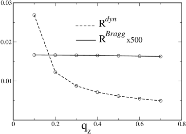
Figure 8: Ratios $R^{Bragg}$ and $R^{dyn}$ for elastic and inelastic orbital to spin scattering, respectively.

Using $|t|=0.5\;eV$ we obtain from Eq.(13) $|t_{eff}|\sim 0.07\;eV$, which yields togther with $a=3.856$ Å  $A\sim 0.09$ for our doping $\delta=0.077$. Comparison of Eq.(14) with Eq.(20) gives

$$\langle\rho_{5}^{\prime}({\bf Q})\rangle\langle\rho^{\dagger}_{5}({\bf Q})\rangle={{\Phi}^{2}\over{2J}}\sim 0.082,$$ (46)

for $T=0$ and $\delta=0.077$. Furthermore, from Eq.(35) we get

$$\langle(B_{5}({\bf Q}))^{2}\rangle_{av}=8/\pi^{2},$$ (47)

which yields

$$R^{Bragg}(0)=3\cdot 10^{-5}.$$ (48)

Unlike in the case of spin scattering the momentum and frequency sums in Eq.(43) are non-trivial and we have carried them out by numerical methods.

Fig. 8 shows the results for $R^{dyn}$ and $R^{Bragg}$ as a function of $q_{z}$ at zero temperature. As expected $R^{dyn}$ increases strongly at small $q_{z}$ due to its logarithmic singularity at $q_{z}=0$. Integrating $R^{dyn}$ also over $q_{z}$ yields a value of about $10^{-2}$ which is more than 2 orders of magnitude larger than $R^{Bragg}$. The reason for this large difference is due to the fact that in the momentum integration in $R^{dyn}$ mainly the small momenta contribute where $1/{\bf q}^{2}$ is larger than 1. In contrast to that, $R^{Bragg}$ probes the integrand of $R^{dyn}$ at the large value $|{\bf Q}|$ where $1/{\bf q}^{2}$ is very small. The extreme small value $R^{Bragg}\sim 10^{-5}$ casts doubts on the identification of the observed Bragg peak at $\bf Q$ with the Bragg peak due a DDWMook . On the other hand, if a DDW state is realized in some material we think that the resulting strong forward scattering peak in neutron scattering would be observable. According to our predictions it would exhaust roughly 3 per cent of the sum rule for spin scattering and thus be of the same order of magnitude as the recently detected elastic scattering from weak magnetic moments directed at least partially perpendicular to the layersBourges in high-$T_{c}$ superconductors.

IV Conclusions

The excitation spectrum of the $t$-$J$ model at large $N$ was studied for dopings where a DDW forms below a transition temperature $T^{\star}$. The density response includes “conventional” local density fluctuations, characterized by the energy scale $t$, where practically all spectral weight is concentrated in a collective sound wave with approximately a sinusoidal dispersion. In addition, and this was the main topic of this investigation, there is a “unconventional” density response from orbital fluctuations caused by fluctuating circulating currents above $T^{\star}$ and fluctuations around a staggered flux phase below $T^{\star}$. The corresponding spectra are again mainly collective, their energy scale is $J$ or a fraction of it, and they can be viewed as order parameter modes of the DDW. At small momentum transfers the spectra are dominated by one well-defined peak corresponding to amplitude fluctuations of the DDW. For larger momentum transfers, unconventional density fluctuations tend to become broad and their intensity suppressed. This is especially true near the point X where practically no weight is left for orbital fluctuations at low frequencies, but instead a rather sharp peak due to sound waves appear at large frequencies reflecting the coupling of the two kinds of density fluctuations.

In principle the above orbital fluctuations show up in the Raman, X-ray and neutron scattering spectra. The predicted scattering intensities are, however, rather small. The reason for this is that, on the one hand, a rather small effective nearest-neighbor hopping element $t_{eff}$ is needed to provide a sufficiently large density of states and the instability to the DDW, on the other hand, the square of $t_{eff}$ appears as a prefactor in the various cross sections due to the Peierls substitution. As a result, the $\bf q$ integrated inelastic cross section is only a few per cents of that for spin scattering and the elastic scattering from the Bragg peak is even much weaker. From our calculations it is also evident that a DDW state in the unconstrained, weak-coupling case would have very similar properties as in the $t$-$J$ model. In particular, the curves for $R^{dyn}$ and $R^{Bragg}$ would closely resemble those in Fig.8. An experimental verification of a DDW state via inelastic neutrons seems to be not unfeasible because a good deal of the scattering intensity is concentrated in a well-pronounced, inelastic peak somewhat smaller than the DDW gap and in small region around the origin in $\bf k$ space.

Acknowledgements The authors are grateful to M. Geisler and T. Enss for help with the figures, H. Yamase for useful discussions, and D. Manske for a critical reading of the manuscript.

References

- (1) B. Dra, K. Maki, and A. Virosztek, Mod. Phys. Lett. B18, 327 (2004).
- (2) B. Dra, A. Virosztek, and K. Maki, Phys. Rev. B65, 155119 (2002).
- (3) T.C. Hsu, J.B. Marston, and I. Affleck, Phys. Rev. B 43, 2866 (1991).
- (4) E. Cappelluti and R. Zeyher, Phys. Rev. B 59, 6475 (1999).
- (5) L. Benfatto, S. Caprara, C. Di Castro, Eur. Phys. J B17, 95 (2000).
- (6) S. Chakravarty, R.B. Laughlin, D.K. Morr, and C. Nayak, Phys. Rev. B 63, 94503 (2001).
- (7) T.P. Devereaux, G.E.D. McCormack, and J.K. Freericks, Phys. Rev. B 68, 075105 (2003).
- (8) B.I. Halperin and T.M. Rice, in , ed. by F. Seitz, D. Turnbull, and H. Ehrenreich (Academic Press, New York, 1968), vol. 21, p.115.
- (9) K.B. Efetov, Phys. Rev. B 43, 5538 (1991).
- (10) B. Valenzuela, E.J. Nicol, and J.P. Carbotte, Phys. Rev. B 71, 134503 (2005).
- (11) L. Benfatto, S.G. Sharapov, N. Andrenacci, and H. Beck, Phys. Rev. B 71, 104511 (2005).
- (12) D.N. Aristov and R. Zeyher, Phys. Rev. B 72, 115118 (2005).
- (13) L. Benfatto and S. Sharapov, cond-mat/0508695.
- (14) R. Zeyher and A. Greco, Phys. Rev. Lett. 89, 177004 (2002).
- (15) S. Tewari and S. Chakravarty, Phys. Rev. B 66, 054510 (2002).
- (16) R. Zeyher and M.L. Kuli, Phys. Rev. B 54, 8985 (1996).
- (17) R. Zeyher and A. Greco, Eur. Phys. J. B 6, 473 (1998).
- (18) L. Gehlhoff and R. Zeyher, Phys. Rev. B 52, 4635 (1995).
- (19) R. Zeyher and A. Greco, phys. stat. sol.(b) 236, 343 (2003).
- (20) Z. Wang, Int. J. of Mod. Physics B 6, 155 (1992).
- (21) H. Yamase, Phys. Rev. Lett. 93, 266404 (2004).
- (22) Ch. Kittel, “Quantum Theory of Solids”, John Wiley, Inc., New York (1963), p. 382.
- (23) A. Greco and R. Zeyher, Phys. Rev. B 63, 064520 (2001).
- (24) H.A. Mook, P. Dai, S.M. Hayden, A. Hiess, S.-H Lee, and F. Dogan, Phys. Rev. B 69, 134509 (2004).
- (25) B. Fauque, Y. Sidis, V. Hinkov, S. Pailhes, C.T. Lin, X. Chaud, and Ph. Bourges, cond-mat/0509210.