Fingerprints of spin-orbital physics in cubic Mott insulators:
Magnetic exchange interactions and optical spectral weights

Abstract

The temperature dependence and anisotropy of optical spectral weights associated with different multiplet transitions is determined by the spin and orbital correlations. To provide a systematic basis to exploit this close relationship between magnetism and optical spectra, we present and analyze the spin-orbital superexchange models for a series of representative orbital-degenerate transition metal oxides with different multiplet structure. For each case we derive the magnetic exchange constants, which determine the spin wave dispersions, as well as the partial optical sum rules. The magnetic and optical properties of early transition metal oxides with degenerate $t_{2g}$ orbitals (titanates and vanadates with perovskite structure) are shown to depend only on two parameters, viz. the superexchange energy $J$ and the ratio $\eta$ of Hund’s exchange to the intraorbital Coulomb interaction, and on the actual orbital state. In $e_{g}$ systems important corrections follow from charge transfer excitations, and we show that KCuF₃ can be classified as a charge transfer insulator, while LaMnO₃ is a Mott insulator with moderate charge transfer contributions. In some cases orbital fluctuations are quenched and decoupling of spin and orbital degrees of freedom with static orbital order gives satisfactory results for the optical weights. On the example of cubic vanadates we describe a case where the full quantum spin-orbital physics must be considered. Thus information on optical excitations, their energies, temperature dependence and anisotropy, combined with the results of magnetic neutron scattering experiments, provides an important consistency test of the spin-orbital models, and indicates whether orbital and/or spin fluctuations are important in a given compound. [Published in: Phys. Rev. B 72, 214431 (2005).]

I Superexchange and optical excitations at orbital degeneracy

The physical properties of Mott (or charge transfer) insulators are dominated by large on-site Coulomb interactions $\propto U$ which suppress charge fluctuations. Quite generally, the Coulomb interactions lead then to strong electron correlations which frequently involve orbitally degenerate states, such as $3d$ (or $4d$) states in transition metal compounds, and are responsible for quite complex behavior with often puzzling transport and magnetic properties.Ima98 The theoretical understanding of this class of compounds, with the colossal magnetoresistance (CMR) manganites as a prominent example, Dag02 ; Dag03 has substantially advanced over the last decade, Mae04 after it became clear that orbital degrees of freedom play a crucial role in these materials and have to be treated on equal footing with the electron spins, which has led to a rapidly developing field — orbital physics.Tok00 Due to the strong onsite Coulomb repulsion, charge fluctuations in the undoped parent compounds are almost entirely suppressed, and an adequate description of these strongly correlated insulators appears possible in terms of superexchange.And59 At orbital degeneracy the superexchange interactions have a rather rich structure, represented by the so-called spin-orbital models, discovered three decades ago,Kug82 ; Cyr75 and extensively studied in recent years. Fei97 ; Kha98 ; Ole00 ; Ish97 ; Fei99 ; Feh04 ; Kha00 ; Kha01 ; Dima2 ; Ole01

Although this field is already quite mature, and the first textbooks have already appeared,Dag03 ; Mae04 ; Faz99 it has been realized only recently that the magnetic and the optical properties of such correlated insulators with partly filled $d$ orbitals are intimately related to each other, being just different experimental manifestations of the same underlying spin-orbital physics. Kha04 ; Lee05 While it is clear that the low-energy effective superexchange Hamiltonian decides about the magnetic interactions, it is not immediately obvious that the high-energy optical excitations and their partial sum rules have the same roots and may be described by the superexchange as well. In fact, this interrelation between the magnetic and the optical properties makes it necessary to reanalyze the spin-orbital superexchange models, and to extract from them important constraints imposed by the theory on the system parameters. We will show that also the opposite holds — some general rules apply for the magnetic interactions in the correlated insulators with degenerate (or almost degenerate) orbitals, and therefore the magnetic measurements impose constraints on any realistic theory. At the same time, we shall argue that such experiments provide very useful information concerning the orbital order (OO) and the strength of quantum fluctuations in a given compound, which can next be employed to interpret other experiments, including the optical spectroscopy.

The phenomena discussed in the present paper go well beyond the more familiar situation of a Mott insulator without orbital degeneracy, or when the orbital degeneracy is lifted by strong Jahn-Teller (JT) distortions as for example in the high $T_{c}$ cuprate superconductors. In a Mott insulator the optical conductivity is purely incoherent, and the optical response is found at energies which exceed the optical gap. When orbital degrees of freedom are absent, the optical gap is determined by the intraorbital Coulomb interaction element $U$. Naively, one might expect that the high-energy charge excitations at energy $\sim U$, which contribute to the optical intensities, are unrelated to the low-energy magnetic phenomena. However, both energy scales are intimately related as the superexchange follows from the same charge excitations which are detected by the optical spectroscopy. The prominent example of this behavior is the nondegenerate Hubbard model, where the virtual high-energy excitations determine the superexchange And59 energy $J$ — it decides, together with spin correlations, about the spectral weight of the upper Hubbard band at half-filling.Bae86 ; Esk94 When temperature increases to an energy scale $\sim J$, the spin correlations are modified and the total spectral weight in the optical spectroscopy follows these changes. Aic02

The superexchange models for transition metal perovskites with partly filled degenerate orbitals have a more complex structure than for nondegenerate orbitals and allow both for antiferromagnetic (AF) and for ferromagnetic (FM) superexchange.Kug82 ; Cyr75 These different contributions to the superexchange result from the multiplet structure of excited transition metal ions which depends on the Hund’s exchange $J_{H}$ and generates a competition between high-spin and low-spin excitations. The exchange interactions are then intrinsically frustrated even on a cubic lattice, which enhances quantum effects both for $e_{g}$, Fei97 ; Kha98 ; Ole00 and for $t_{2g}$ systems.Kha00 ; Kha01 This frustration is partly removed in anisotropic AF phases, which break the cubic symmetry and effectively may lead to dimensionality changes, such as in $A$-type AF phase realized in LaMnO₃, or in $C$-type AF phase in LaVO₃.

While rather advanced many-body treatment of the quantum physics characteristic for spin-orbital models is required in general, we want to present here certain simple principles which help to understand the heart of the problem and give simple guidelines for interpreting experiments and finding relevant physical parameters of the spin-orbital models of undoped cubic insulators. We will argue that such an approach based upon classical OO is well justified in many known cases, as quantum phenomena are often quenched by the Jahn-Teller (JT) coupling between orbitals and the lattice distortions, which are present below structural phase transitions and induce OO both in spin-disordered and in spin-ordered phases. Kan59 However, we will also discuss the prominent example of LaVO₃, where assuming perfect OO or attempts to decouple spin and orbital fluctuations,Mot03 fail in a spectacular way and give no more than a qualitative insight into certain limiting cases. Significant corrections due to quantum phenomena that go beyond such simplified approaches are then necessary for a more quantitative understanding.

In the correlated insulators with partly occupied degenerate orbitals not only the structure of the superexchange is complex, but also the optical spectra exhibit strong anisotropy and temperature dependence near the magnetic transitions, as found in LaMnO₃, Tob01 ; Kov04 the cubic vanadates LaVO₃ and YVO₃, Miy02 ; Tsv04 and in the ruthenates.Lee02 In all these systems several excitations contribute to the excitation spectra, so one may ask how the spectral weight redistributes between individual subbands originating from these excitations. The spectral weight distribution is in general anisotropic already when OO sets in and breaks the cubic symmetry, but even more so when $A$-type or $C$-type AF spin order occurs below the Néel temperature.

The effective spin-orbital models of transition metal oxides with partly filled degenerate orbitals depend in a characteristic way upon those aspects of the electronic structure which decide whether a given strongly correlated system can be classified as a Mott insulator or as a charge transfer (CT) insulator. As suggested in the original classification of Zaanen, Sawatzky and Allen,Zaa85 the energy of the $d-p$ CT excitation $\Delta$ has to be compared with the Coulomb interaction $U$ — if $U<\Delta$, the first excitation is at a transition metal ion and the system is a Mott insulator, otherwise it is a CT insulator. Both are strongly correlated insulators, yet in one limit the dominant virtual excitations are of $d-d$ type, whereas in the other limit they are of $p-d$ type. One may consider this issue more precisely by analyzing the full multiplet structure, and comparing the lowest excitation energy (to a high-spin configuration) at a transition metal ion, $\varepsilon_{\rm HS}=U-3J_{H}$, with that of the lowest CT excitation (of energy $\Delta$) between a transition metal ion and a ligand ion. notede Thus we argue that one can regard a given perovskite as a charge transfer insulator if $\varepsilon_{\rm HS}>\Delta$, and as a Mott-Hubbard insulator if $\varepsilon_{\rm HS}<\Delta$. By analyzing these parameters it has been suggested that the late transition metal oxides may be classified as CT insulators.Ima98 In this case important new contributions to the superexchange arise, Goode ; Zaa88 ; Mos04 called below $\Delta$ (charge transfer) terms, as we shall discuss for two $e_{g}$ systems: KCuF₃ and LaMnO₃.

A central aim of this paper is to provide relatively simple expressions for the magnetic exchange constants and for the optical spectral weights that can be used by experimentalists to analyze and compare their spin wave data with optical data. While the full spin-orbital models are rather complex, they are nevertheless controlled by only very few physical parameters: (i) the superexchange constant $J$, (ii) the normalized Hund’s exchange $\eta$, and (iii) the charge transfer parameter $R$. There are two distinct ways to determine these effective parameters: either (i) from the original multiband Hubbard model, or (ii) from experimental spin wave and/or optical data. Here the second approach is of particular interest because the simultaneous analysis of magnetism and optics provides a subtle test of the underlying model.

The paper is organized as follows. In Sec. II we introduce the generic structure of the low-energy effective Hamiltonian in a correlated insulator with orbital degeneracy, and discuss its connection with the optical excitations at high-energy. This general formulation provides the important subdivision of a given spin-orbital model which is necessary to obtain the partial spectral weights for individual multiplet transitions. In the remaining part of the paper we concentrate on some selected cubic perovskites and demonstrate that this general formulation allows one to arrive at a consistent interpretation of the magnetic and optical experiments in these correlated insulators using the superexchange interactions (Secs. III-VI), and to deduce the parameters relevant for the theoretical model from the experimental data, whereever available. We start in Sec. III with the simplest spin-orbital model for $e_{g}$ holes in KCuF₃, and demonstrate that this system is in the CT regime which changes the commonly used picture of superexchange in this system in a qualitative way. Next we present and analyze the spin-orbital model with $e_{g}$ orbital degrees of freedom for the undoped manganite LaMnO₃ in Sec. IV. Here we show that in this case much smaller contributions arise from the CT processes, and the system is already in the Mott-Hubbard regime of parameters, which explains the earlier success of a simplified effective model based entirely on $d-d$ excitations and sufficient for a semiquantitative understanding. This justifies our approach to the early transition metal perovskites with $t_{2g}$ degrees of freedom, titanates in Sec. V and vanadates in Sec. VI, which we treat as Mott-Hubbard insulators. For all these systems we analyze the magnetic exchange interactions and the optical spectral weights, depending on the nature of the spin correlations in the ground state. The paper is concluded in Sec. VII, where we provide a coherent view on the magnetic and the optical phenomena and summarize the experimental constraints on the model parameters.

II General formalism

We consider here effective models with hopping elements between transition metal ions,

$$H_{0}=\sum_{i\alpha\sigma}\varepsilon_{i\alpha}n_{i\alpha\sigma}+\sum_{ij,\alpha\neq\beta,\sigma}t_{i\alpha,j\beta}a_{i\alpha\sigma}^{\dagger}a_{j\beta\sigma}.$$ (1)

Here $\varepsilon_{i\alpha}$ are orbital energies, and $t_{i\alpha,j\beta}$ are effective hopping elements via ligand orbitals — they depend on the type of considered orbitals as discussed in Refs. And78, and Zaa93, . The energy scale for the hopping is set by the largest hopping element $t$: the $(dd\sigma)$ element in case of $e_{g}$ systems, and the $(dd\pi)$ element when only $\pi$ bonds are considered in systems with degenerate and partly filled $t_{2g}$ orbitals. For noninteracting electrons the Hamiltonian $H_{0}$ would lead to tight-binding bands, but in a Mott insulator the large Coulomb interaction $U$ suppresses charge excitations in the regime of $U\gg t$, and the hopping elements can only contribute via virtual excitations, leading to the superexchange.

The superexchange in the $3d$ cubic systems with orbital degeneracy is described by spin-orbital models, where both degrees of freedom are coupled and the orbital state (ordered or fluctuating) determines the spin structure and excitations, and vice versa. The numerical and analytical structure of these models represents a fascinating challenge in the theory, as it is much more complex than that of pure spin models. The spin-orbital models have been derived before in several cases, and we refer for these derivations to the original literature.Ole00 ; Fei99 ; Kha00 ; Kha01 They describe in low energy regime the consequences of virtual charge excitations between two neighboring transition metal ions, $d_{i}^{m}d_{j}^{m}\rightleftharpoons d_{i}^{m+1}d_{j}^{m-1}$, which involve an increase of energy due to the Coulomb interactions. Such transitions are mediated by the ligand orbitals between the two ions and have the same roots as the superexchange in a Mott insulator with nondegenerate orbitalsAnd59 at $U\gg t$ — thus the resulting superexchange interactions will be called $U$ terms. The essential difference which makes it necessary to analyze the excitation energies in each case separately is caused by the existence of several different excitations. Their energies have to be determined first by analyzing the eigenstates of the local Coulomb interactions,

$$H_{int} = U\sum_{i\alpha}n_{i\alpha\uparrow}n_{i\alpha\downarrow}+\sum_{i,\alpha<\beta}\Big{(}U_{\alpha\beta}-\frac{1}{2}J_{\alpha\beta}\Big{)}n_{i\alpha}n_{i\beta}$$ (2)

$$+ \sum_{i,\alpha<\beta}J_{\alpha\beta}\Big{(}d^{\dagger}_{i\alpha\uparrow}d^{\dagger}_{i\alpha\downarrow}d_{i\beta\downarrow}d_{i\beta\uparrow}+d^{\dagger}_{i\beta\uparrow}d^{\dagger}_{i\beta\downarrow}d_{i\alpha\downarrow}d_{i\alpha\uparrow}\Big{)}$$

$$- 2\sum_{i,\alpha<\beta}J_{\alpha\beta}\textbf{S}_{i\alpha}\cdot\textbf{S}_{i\beta},$$

with $\bar{\sigma}=-\sigma$, which in the general case depend on the three Racah parameters $A$, $B$ and $C$,Gri71 which may be derived from somewhat screened atomic values. While the intraorbital Coulomb element

$$U=A+4B+3C,\\$$ (3)

is identical for all $3d$ orbitals, the interorbital Coulomb and exchange elements, $U_{\alpha\beta}$ and $J_{\alpha\beta}$, are anisotropic and depend on the involved pair of orbitals; the values of $J_{\alpha\beta}$ are given in Table 1. The Coulomb and exchange elements are related to the intraorbital element $U$ by a relation which guarantees the invariance of interactions in the orbital space,

$$U=U_{\alpha\beta}+2J_{\alpha\beta}.$$ (4)

Table 1: On-site interorbital exchange elements $J_{\alpha\beta}$ for $3d$ orbitals as functions of the Racah parameters $B$ and $C$ (for more details see Ref. Gri71, ).

orbital	$xy$	$yz$	$zx$	$x^{2}\!-\!y^{2}$	$3z^{2}\!-\!r^{2}$
$xy$	$0$	$3B+C$	$3B+C$	$C$	$4B+C$
$yz$	$3B+C$	$0$	$3B+C$	$3B+C$	$B+C$
$zx$	$3B+C$	$3B+C$	$0$	$3B+C$	$B+C$
$x^{2}\!-\!y^{2}$	$C$	$3B+C$	$3B+C$	$0$	$4B+C$
$3z^{2}\!-\!r^{2}$	$4B+C$	$B+C$	$B+C$	$4B+C$	$0$

In cases where only the orbitals of one type ($e_{g}$ or $t_{2g}$) are partly filled, however, as e.g. in the titanates, vanadates, or copper fluorides, all relevant exchange elements $J_{\alpha\beta}$ are the same (see Table 1) and one may use a simplified form of onsite interactions,Ole83

$$H_{int}^{(0)} = U\sum_{i\alpha}n_{i\alpha\uparrow}n_{i\alpha\downarrow}+\Big{(}U-\frac{5}{2}J_{H}\Big{)}\sum_{i,\alpha<\beta}n_{i\alpha}n_{i\beta}$$ (5)

$$+ J_{H}\sum_{i,\alpha<\beta}\Big{(}d^{\dagger}_{i\alpha\uparrow}d^{\dagger}_{i\alpha\downarrow}d_{i\beta\downarrow}d_{i\beta\uparrow}+d^{\dagger}_{i\beta\uparrow}d^{\dagger}_{i\beta\downarrow}d_{i\alpha\downarrow}d_{i\alpha\uparrow}\Big{)}$$

$$- 2J_{H}\sum_{i,\alpha<\beta}\textbf{S}_{i\alpha}\cdot\textbf{S}_{i\beta}.$$

with only two parameters: the Coulomb element $U$ (3) and a Hund’s exchange element $J_{H}$, being $4B+C$ for $e_{g}$ and $3B+C$ for $t_{2g}$ systems, respectively. We emphasize that in the general case when both types of orbitals are partly filled (as in the manganites) and both thus participate in charge excitations, the Hamiltonian (5) is only approximate, and the full excitation spectra of the transition metal ionsGri71 which follow from Eq. (2) have to be used instead. A few examples of spectra for $d_{i}^{m}d_{j}^{m}\rightleftharpoons d_{i}^{m+1}d_{j}^{m-1}$ charge excitations at transition metal ions are shown in Fig. 1. As a universal feature, the high-spin excitation is found at energy $U-3J_{H}$ in all cases, provided that $J_{H}$ is understood as Hund’s exchange for that partly filled manifold ($e_{g}$ or $t_{2g}$) of degenerate $d$ orbitals which participate in charge excitations. The structure of the excited states depends on the partly occupied orbitals noteabc and on the actual valence $m$ — the distance between the high-spin and low-spin excitations increases with the number of electrons for $m\leq 5$ (holes for $m>5$).

At orbital degeneracy the superexchange which connects ions at sites $i$ and $j$ along the bond $\langle ij\rangle$ involves orbital operators which depend on the bond direction. Therefore, we introduce the index $\gamma=a,b,c$ to label the three a priori equivalent directions in a cubic crystal. In order to analyze the consequences of each individual charge excitation $n$ that contributes to the superexchange in a given transition metal compound with degenerate $d$ orbitals, we shall use below a general way of writing the effective low-energy Hamiltonian as a superposition of such individual terms on each bond $\langle ij\rangle$,

$${\cal H}_{U}=\sum_{n}\sum_{\langle ij\rangle\parallel\gamma}H_{n}^{(\gamma)}(ij),$$ (6)

with the energy unit [absorbed in individual $H_{n}^{(\gamma)}(ij)$ terms] given by the superexchange constant,

$$J=\frac{4t^{2}}{U}.$$ (7)

It follows from $d-d$ charge excitations with an effective hopping element $t$ between transition metal ions, and is the same as that obtained in a Mott insulator with nondegenerate orbitals in the regime of $U\gg t$.And59 While $U$ is the uniquely defined on-site intraorbital Coulomb element (3), increasing upon going from Ti to Cu along the transition metal series,vdM88 ; Miz96 the definition of the hopping $t$ between two nearest neighbor transition metal ions depends on the system.Zaa93 If degenerate $e_{g}$ orbitals are involved, it is the effective $(dd\sigma)$ hopping element for a $\sigma$-bond which involves $p_{\sigma}$ orbitals on the intervening ligand ion (e.g. for the hopping between two directional $3z^{2}-r^{2}$ states along the $c$ axis), while for the systems with degenerate $t_{2g}$ orbitals it stands for the effective $(dd\pi)$ hopping element due to $\pi$ bonds which involve $p_{\pi}$ orbitals on the ligand ion.

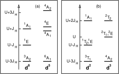
Figure 1: Energies of $d_{i}^{m}d_{j}^{m}\rightarrow d_{i}^{m+1}d_{j}^{m-1}$ charge excitations in selected cubic transition metal oxides, as obtained from Eq. (5) for: (a) $e_{g}$ excitations of Cu³⁺ ($d^{8}$) and Mn²⁺ ($d^{5}$) ions [in the $d^{5}$ case the spectrumnoteabc was obtained from Eq. (2)]; (b) $t_{2g}$ excitations of Ti²⁺ ($d^{2}$) and V²⁺ ($d^{3}$) ions. The splittings between different states are due to Hund’s exchange element $J_{H}$ which refers to a pair of $e_{g}$ electrons in (a), and to a pair of $t_{2g}$ electrons in (b), respectively.

In the superexchange Hamiltonian Eq. (6) the contributions which originate from all possible virtual excitations $d_{i}^{m}d_{j}^{m}\rightleftharpoons d_{i}^{m+1}d_{j}^{m-1}$ just add up to the total superexchange interaction, in which the individual terms cannot be distinguished. Yet each of these excitations involves a different state in the multiplet structure of at least one of the transition metal ions, i.e., either in the $d^{m+1}$ or in the $d^{m-1}$ configuration or in both, depending on the actual process and on the value of $m$. As pointed out elsewhere,Kha04 the same charge excitations contribute to the optical conductivity, and here they appear at distinct energies, thus revealing the multiplet structure of the excited transition metal ions. Moreover, they convey a rich and characteristic temperature dependence to the optical spectrum, determined by the temperature variation of the spin-spin and orbital-orbital correlations. We emphasize that it is therefore important to analyze the various multiplet excitations separately, as they depend on these correlations in a different way, and will also contribute to a quite different temperature dependence, as we show in this paper on several examples.

As we will see in more detail below, the generic structure of each such individual contribution is for a bond $\langle ij\rangle$ given by

$$H_{n}^{(\gamma)}(ij) = (a_{n}+b_{n}\>{\vec{S}}_{i}\cdot{\vec{S}}_{j})\>Q_{n}^{(\gamma)}({\vec{\tau}}_{i},{\vec{\tau}}_{j})$$ (8)

$$= a_{n}Q_{n}^{(\gamma)}({\vec{\tau}}_{i},{\vec{\tau}}_{j})$$

$$+b_{n}\>Q_{n}^{(\gamma)}({\vec{\tau}}_{i},{\vec{\tau}}_{j})\>{\vec{S}}_{i}\cdot{\vec{S}}_{j},$$

where the orbital dependence of the superexchange is described by means of orbital projection operators $Q_{n}^{(\gamma)}$ which are expressed in terms of components of orbital pseudospin $T=1/2$ operators at sites $i$ and $j$. The coefficients $a_{n}$ and $b_{n}$, which measure the strength of the purely orbital part and of the spin-and-orbital part of the superexchange, respectively, follow from second-order perturbation theory involving the charge excitation $n$. In the present case of perovskites, where the bond between two transition metal ions through the ligand ion (F or O) connecting them is close to linear (180^∘), the coefficients $a_{n}$ and $b_{n}$ are of similar magnitude (in contrast to the situation in layered compounds like LiNiO₂ with 90^∘ bonds where the purely orbital interaction is stronger by an order of magnitude than the spin-and-orbital interactionMos02 ).

Here we consider systems having cubic symmetry at high temperature. Yet at low temperature this symmetry is frequently spontaneously broken — usually driven by the joint effect of (i) the orbital part of the superexchange interaction, and (ii) the JT coupling of the same degenerate (and therefore JT active) $3d$ orbitals to lattice modes. The result is the simultaneous onset of a macroscopic lattice distortion and of OO, i.e., a cooperative JT effect. At temperatures well below the transition temperature $T_{s}$ of this combined structural and orbital phase transition, the OO is effectively frozen. The remaining superexchange interactions between the spins may then be obtained by replacing the orbital projection operators in Eq. (6) by their expectation values,

$$Q_{n}^{(\gamma)}({\vec{\tau}}_{i},{\vec{\tau}}_{j})\longrightarrow\langle Q_{n}^{(\gamma)}({\vec{\tau}}_{i},{\vec{\tau}}_{j})\rangle=Q_{n}^{(\gamma)}(\langle{\vec{\tau}}_{i}\rangle,\langle{\vec{\tau}}_{j}\rangle).$$ (9)

Obviously, this leads to anisotropic magnetic interactions,

$$H_{s}=J\sum_{n}\sum_{\langle ij\rangle\parallel\gamma}b_{n}\>\langle Q_{n}^{(\gamma)}\rangle\>{\vec{S}}_{i}\cdot{\vec{S}}_{j},$$ (10)

which will in general induce a further magnetic phase transition at lower temperature. It is noteworthy that in this situation the spin degrees of freedom get decoupled from the orbital degrees of freedom, although the purely orbital ($a_{n}$) and spin-and-orbital ($b_{n}$) superexchange terms are of similar strength. Responsible for this behavior is the JT contribution to the structural phase transition, which enhances $T_{s}$ above the value it would have if the transition were driven by orbital superexchange alone.

Starting from the microscopic spin-orbital superexchange models, we will analyze the effective spin models which arise after such a symmetry breaking at low temperature. Rewritten from Eq. (10), they are of the generic form

$$H_{s}=J_{c}\sum_{\langle ij\rangle_{c}}{\vec{S}}_{i}\cdot{\vec{S}}_{j}+J_{ab}\sum_{\langle ij\rangle_{ab}}{\vec{S}}_{i}\cdot{\vec{S}}_{j},$$ (11)

with two different effective magnetic exchange interactions: $J_{c}$ along the $c$ axis, and $J_{ab}$ within the $ab$ planes. The latter $J_{ab}$ interactions could in principle still take two different values in case of inequivalent lattice distortions (caused, e.g., by octahedra tilting or pressure effects) making the $a$ and $b$ axes inequivalent, but we intend to limit the present analysis to idealized structures with these two axes being equivalent. We shall show that the spin-spin correlations along the $c$ axis and within the $ab$ planes,

$$s_{c}=\langle\vec{S}_{i}\cdot\vec{S}_{j}\rangle_{c},\hskip 19.91684pts_{ab}=\langle\vec{S}_{i}\cdot\vec{S}_{j}\rangle_{ab},$$ (12)

next to the orbital correlations, play an important role in the intensity distribution in optical spectroscopy.

The spectral weight in the optical spectroscopy is determined by the kinetic energy,Mal77 and reflects the onset of magnetic order Cha00 ; Mil00 and/or orbital order.Mac99 As shown by Ahn and Millis,Mil00 in the weak coupling regime one can analyze the total spectral weight in optical absorption using the Hartree-Fock approximation for the relevant tight-binding Hamiltonian. In a correlated insulator the electrons are almost localized and the only kinetic energy which is left is associated with the same virtual charge excitations that contribute also to the superexchange. Therefore, we will discuss here the individual kinetic energy terms $K_{n}^{(\gamma)}$, which can be determined from the superexchange (6) using the Hellman-Feynman theorem,Bae86

$$K_{n}^{(\gamma)}=-2\big{\langle}H_{n}^{(\gamma)}(ij)\big{\rangle}.$$ (13)

For convenience, we define the $K_{n}^{(\gamma)}$ as positive quantities. Making use of the generic form of the superexchange contribution $H_{n}^{(\gamma)}(ij)$ given by Eq. (8), and assuming as above that spin and orbital degrees of freedom are decoupled in the temperature range of interest, we obtain

$$K_{n}^{(\gamma)}=-2J\big{(}a_{n}+b_{n}\>\langle{\vec{S}}_{i}\cdot{\vec{S}}_{j}\rangle_{\gamma}\big{)}\>\big{\langle}Q_{n}^{(\gamma)}({\vec{\tau}}_{i},{\vec{\tau}}_{j})\big{\rangle}.$$ (14)

Each term $K_{n}^{(\gamma)}$ (13) originates from a given charge excitation $n$ for a bond $\langle ij\rangle$ along axis $\gamma$. These terms are directly related to the partial optical sum rule for individual Hubbard bands, which readsKha04

$$\frac{a_{0}\hbar^{2}}{e^{2}}\int_{0}^{\infty}\sigma_{n}^{(\gamma)}(\omega)d\omega=\frac{\pi}{2}K_{n}^{(\gamma)},$$ (15)

where $\sigma_{n}^{(\gamma)}(\omega)$ is the contribution of band $n$ to the optical conductivity for polarization along the $\gamma$ axis, $a_{0}$ is the distance between transition metal ions, and the tight-binding model with nearest neighbor hopping is implied. Comparison with Eq. (14) shows that the intensity of each band is indeed determined by the underlying OO together with the spin-spin correlation along the direction corresponding to the polarization.

One has to distinguish the above partial sum rule (15) from the sum rule for the total spectral weight in the optical spectroscopy for polarization along a cubic direction $\gamma$, involving

$$K^{(\gamma)}=-2J\sum_{n}\big{\langle}H_{n}^{(\gamma)}(ij)\big{\rangle},$$ (16)

which stands for the total intensity in the optical excitations (due to $d-d$ excitations). This quantity is of less interest here as it has a much weaker temperature dependence and does not allow for a direct insight into the nature of the electronic structure. In addition, it might be also more difficult to resolve from experiment.

When the low-energy excitations are of CT type, two holes could also be created within a $2p$ orbital on a ligand (oxygen or fluorine) ion in between two transition metal ions, described by $d_{i}^{m}p^{6}d_{j}^{m}\rightleftharpoons d_{i}^{m+1}p^{4}d_{j}^{m+1}$ processes — these CT contributions lead to additional superexchange contributions, called below $\Delta$ terms. While the latter terms can be safely neglected in Mott-Hubbard systems, they substantially modify the superexchange in CT insulators, and may even represent there the dominating contribution.Zaa88 ; Mos04 Below we will analyze them in two situations which involve $e_{g}$ degrees of freedom, viz. in the cubic copper fluoride KCuF₃ (Sec. III), and in the cubic manganite LaMnO₃ (Sec. IV), and we will show that in KCuF₃ they represent an essential part of the superexchange.

III Copper fluoride perovskite: KCuF₃

III.1 Superexchange Hamiltonian

The simplest spin-orbital models are obtained when transition metal ions are occupied by either one electron ($m=1$), or by nine electrons ($m=9$); in these cases the Coulomb interactions (5) contribute only in the excited state (in the $d^{2}$ or the $d^{8}$ configuration) after a charge excitation $d_{i}^{m}d_{j}^{m}\rightleftharpoons d_{i}^{m+1}d_{j}^{m-1}$ between two neighboring ions. Here we start with the case of a single hole in the $d$ shell, as realized for the Cu²⁺ ions in KCuF₃ with the $d^{9}$ configuration ($m=9$). Due to the splitting of the $3d$ states in the octahedral field within the CuF₆ octahedra, the hole at each magnetic Cu²⁺ ion occupies one of the $e_{g}$ orbitals. The superexchange coupling (6) is usually analyzed in terms of $e_{g}$ holes in this case,Kug82 and this has become a textbook example of spin-orbital physics by now.Faz99 ; Mae04

Orbital order occurs in KCuF₃ below the structural transition at $T_{s}\sim 800$ K. At $T<T_{s}$ the structure is tetragonal, with longer Cu$-$Cu distances within the $ab$ planes ($d_{ab}=8.28$ Å) than along the $c$ axis ($d_{c}=7.85$ Å),Kad67 which favors strong AF interactions along the $c$ axis. Below the magnetic transition at $T_{N}\simeq 38$ K, long-range magnetic order of $A$-type sets in, Sat80 ; Pao02 and the ordered moment is $\mu_{0}=0.48\mu_{B}$. Hut69

The superexchange between the Cu²⁺ ions in KCuF₃,

$${\cal H}(d^{9})={\cal H}_{U}(d^{9})+{\cal H}_{\Delta}(d^{9}),$$ (17)

consists of two terms: the $U$ term ${\cal H}_{U}$ (6), and the CT term ${\cal H}_{\Delta}$. First we introduce the $U$ term ${\cal H}_{U}(d^{9})$ following the general approach of Sec. II. It originates from three different excitations, leading to an intermediate $d^{8}$ configuration at an excited Cu³⁺ ion. Using the model Hamiltonian (5) to describe the Coulomb interactions between the $e_{g}$ electrons, one finds an equidistant excitation spectrum of ${}^{3}\!A_{2}$, ${}^{1}E$ (${}^{1}E_{\theta}$ and ${}^{1}E_{\epsilon}$) and ${}^{1}\!A_{1}$ states, with energies:Gri71 ; Ole00 $U-3J_{H}$, $U-J_{H}$ and $U+J_{H}$, as shown in Fig. 1(a). This excitation spectrum is exact, and the element $J_{H}$ for a pair of $e_{g}$ electrons is given by the Racah parameters $B$ and $C$ (see Table I):

$$J_{H}=4B+C.$$ (18)

This definition of $J_{H}$ will be used for two systems with $e_{g}$ orbital degrees of freedom: for the copper fluoride KCuF₃ (considered here), and for the manganite LaMnO₃ (in Sec. IV).

In what follows, we will parametrize the multiplet structure of the different transition metal ions by the ratio of the Hund’s element $J_{H}$ and the intraorbital Coulomb element $U$,

$$\eta=\frac{J_{H}}{U}.$$ (19)

Using Eqs. (6) and (19), one finds for each bond $\langle ij\rangle$ along a $\gamma$ axis ($\gamma=a,b,c$) four contributions:Ole00

$$H_{1}^{(\gamma)}\!\! = -\frac{J}{2}r_{1}\Big{(}\vec{S}_{i}\!\cdot\!\vec{S}_{j}+\frac{3}{4}\Big{)}\Big{(}\frac{1}{4}-\!\tau_{i}^{(\gamma)}\tau_{j}^{(\gamma)}\Big{)},$$ (20)

$$H_{2}^{(\gamma)}\!\! = \!\frac{J}{2}r_{2}\Big{(}\vec{S}_{i}\!\cdot\!\vec{S}_{j}-\frac{1}{4}\Big{)}\Big{(}\frac{1}{4}-\!\tau_{i}^{(\gamma)}\tau_{j}^{(\gamma)}\Big{)},$$ (21)

$$H_{3}^{(\gamma)}\!\! = \!\frac{J}{2}r_{3}\Big{(}\vec{S}_{i}\!\cdot\!\vec{S}_{j}-\frac{1}{4}\Big{)}\!\Big{(}\frac{1}{2}-\!\tau_{i}^{(\gamma)}\Big{)}\!\Big{(}\frac{1}{2}-\!\tau_{j}^{(\gamma)}\Big{)},$$ (22)

$$H_{4}^{(\gamma)}\!\! = \!\frac{J}{2}r_{4}\Big{(}\vec{S}_{i}\!\cdot\!\vec{S}_{j}-\frac{1}{4}\Big{)}\!\Big{(}\frac{1}{2}-\!\tau_{i}^{(\gamma)}\Big{)}\!\Big{(}\frac{1}{2}-\!\tau_{j}^{(\gamma)}\Big{)},$$ (23)

with coupled spin and orbital operators. The coefficients,

$$r_{1}=\frac{1}{1-3\eta},\hskip 5.69046ptr_{2}=r_{3}=\frac{1}{1-\eta},\hskip 5.69046ptr_{4}=\frac{1}{1+\eta},$$ (24)

follow from the above multiplet structure of $d^{8}$ ions.notejt

As explained below, it is straightforward to understand the generic structure of the superexchange term ${\cal H}_{U}$, given by Eqs. (20)–(23). Here $\vec{S}_{i}$ is a spin $S=1/2$ operator, and

$$P_{1}(ij)=\vec{S}_{i}\!\cdot\!\vec{S}_{j}+\frac{3}{4},\hskip 19.91684ptP_{0}(ij)=\frac{1}{4}-\vec{S}_{i}\!\cdot\!\vec{S}_{j},$$ (25)

are the spin projection operators on triplet ($S=1$) and singlet ($S=0$) spin states for a bond $\langle ij\rangle$, so one recognizes the high-spin term (20) and three low-spin terms (21)–(23), respectively. The spin operators in Eqs. (20)–(23) are accompanied by orbital pseudospin operators $\propto\tau_{i}^{(\gamma)}$, which select the type of orbitals occupied by holes at sites $i$ and $j$, and simultaneously dictate the allowed excited states.

The orbital operators $\tau_{i}^{(\gamma)}$ depend on the direction of a considered bond $\langle ij\rangle$, and are given by

$$\tau^{(ab)}_{i}=-\frac{1}{4}\big{(}\sigma^{z}_{i}\mp\sqrt{3}\sigma^{x}_{i}\big{)},\hskip 19.91684pt\tau^{(c)}_{i}=\frac{1}{2}\sigma^{z}_{i},$$ (26)

where $\sigma^{z}_{i}$ and $\sigma^{x}_{i}$ are Pauli matrices acting on the orbital pseudospins and the signs $\pm$ in $\tau^{(ab)}_{i}$ correspond to $a$ and $b$ axis, respectively. With the help of $\tau^{(\gamma)}_{i}$ one defines next the projection operators in the orbital subspace,

$${\cal Q}_{i\xi}^{(\gamma)}=\frac{1}{2}+\tau_{i}^{(\gamma)},\hskip 19.91684pt{\cal Q}_{i\zeta}^{(\gamma)}=\frac{1}{2}-\tau_{i}^{(\gamma)}.\hskip 19.91684pt$$ (27)

For a given cubic axis $\gamma$ they project (at site $i$) either on the planar orbital $|\xi\rangle$ in the plane perpendicular to the $\gamma$ axis, or on the orthogonal directional orbital $|\zeta\rangle$ along this axis. For instance, in the case where $\gamma$ is the $c$ axis, they project on the $x^{2}-y^{2}$ orbital in the $ab$ plane, and on the directional $3z^{2}-r^{2}$ orbital along the $c$ axis.

Using the projection operators (27), the orbital dependence in Eqs. (20)-(23) becomes transparent. First of all, $(\frac{1}{4}-\tau_{i}^{(\gamma)}\tau_{j}^{(\gamma)})$ in Eq. (20) accompanies the high-spin ${}^{3}\!A_{2}$ excitation as this state may occur only when a pair of orthogonal orbitals is occupied at sites $i$ and $j$, described formally by a superposition of two possibilities, $\frac{1}{2}({\cal Q}_{i\zeta}{\cal Q}_{j\xi}+{\cal Q}_{i\xi}{\cal Q}_{j\zeta})$. In contrast, the operator ${\cal Q}_{i\zeta}{\cal Q}_{j\zeta}$ selects two orbitals oriented along the bond $\langle ij\rangle$ for the high-energy low-spin ${}^{1}\!A_{1}$ excitation, see Eq. (23). Finally, the second $H_{2}^{(\gamma)}$ (21) and third $H_{3}^{(\gamma)}$ (22) term correspond to the doubly degenerate low-spin ${}^{1}E$ state which consists of two singlet excitations: (i) an interorbital singlet with two different orbitals occupied (${}^{1}E_{\epsilon}$), and (ii) a double occupancy within a directional orbital at either site (${}^{1}E_{\theta}$) — these two excitations have thus quite different orbital dependences, identical with those of the ${}^{3}\!A_{2}$ and the ${}^{1}\!A_{1}$ excitation, respectively. The sum over all the terms $H_{n}^{(\gamma)}$, with $n=1,\cdots,4$, gives the simplest version of the spin-orbital model for the cubic copper fluoride KCuF₃ with degenerate $e_{g}$ orbitals. Its derivation and more details on the classical phase diagram can be found in Ref. Ole00, .

By considering further the electronic structure of KCuF₃, one can elucidate the role played by the CT part ${\cal H}_{\Delta}$ in the superexchange Hamiltonian (17). By analogy with the CuO₂ planes of the high-temperature superconductors, where the CT processes give the dominating contribution to the AF superexchange interaction, Zaa88 ; Zaa90 one expects that they are also important for a cubic copper(II) fluoride and modify the superexchange in KCuF₃. The CT term,

$${\cal H}_{\Delta}(d^{9}) = JR\sum_{\langle ij\rangle\parallel\gamma}\Big{(}\vec{S}_{i}\!\cdot\!\vec{S}_{j}-\frac{1}{4}\Big{)}\Big{(}\frac{1}{2}-\tau_{i}^{(\gamma)}\Big{)}\Big{(}\frac{1}{2}-\tau_{j}^{(\gamma)}\Big{)},$$

with the coefficient

$$R=\frac{2U}{2\Delta+U_{p}}$$ (29)

resulting from the two-hole charge excitation at a common neighboring $2p_{\sigma}$ orbital of a fluorine ion in between two copper ions, in the process $d_{i}^{9}p_{\langle ij\rangle}^{6}d_{j}^{9}\rightleftharpoons d_{i}^{10}p_{\langle ij\rangle}^{4}d_{j}^{10}$. As a double hole excitation is generated at a single bonding orbital $2p_{\sigma}$ within each Cu$-$F$-$Cu unit, this term is necessarily AF. Two holes can move to fluorine from two neighboring Cu ions only if both of them occupy a directional $e_{g}$ orbital $|\zeta\rangle$, oriented along the considered bond (e.g., $3x^{2}-r^{2}$ orbitals along the $a$ axis), being the simplest CT term discussed recently by Mostovoy and Khomskii.Mos04 Therefore this process leads to the same orbital dependence in Eq. (III.1) as the low-spin ${}^{1}E_{\theta}$ and ${}^{1}\!A_{1}$ excitations which involve double occupancies of directional $|\zeta\rangle$ orbitals.

III.2 Spin exchange constants and optical intensities

A characteristic feature of spin-orbital superexchange models with $e_{g}$ orbital degrees of freedom is the presence of the purely orbital interactions in Eqs. (20)–(23) and (III.1), which favor particular type of occupied orbitals. LDA+U calculations Lic95 ; Med02 have indicated that such purely electronic interactions would already drive the instability towards the $C$-type OO ($C$-OO) phase, with alternating orbitals in the $ab$ planes, and repeated orbitals along the $c$ axis, which induces FM spin exchange in the $ab$ planes, and strong AF exchange between the planes. Experimentally, this OO sets in below the structural transition at $T_{s}\sim 800$ K,Pao02 i.e., at much higher temperature than the characteristic energy scale of the magnetic excitations,Ten93 suggesting that the JT effect plays an important role in this instability. This observation is consistent with the large difference between $T_{s}$ and the Néel temperature $T_{N}\sim 38$ K, Hut69 the latter being controlled by the magnetic part of the superexchange, and thus the orbital correlations decouple from the spin-spin correlations. This motivates one to analyze the dependence of the magnetic exchange interactions and of the optical spectral weights on the type of OO stabilized below the structural transition.

Here we are interested in the low temperature range of $T<500$ K, so we assume perfect OO given by a classical ansatz for the ground state,

$$|\Phi_{0}\rangle=\prod_{i\in A}|\theta_{A}\rangle_{i}\prod_{j\in B}|\theta_{B}\rangle_{j},$$ (30)

with the orbital states, $|\theta_{A}\rangle_{i}$ and $|\theta_{B}\rangle_{j}$, characterized by opposite angles ($\theta_{A}=-\theta_{B}$) and alternating between two sublattices $A$ and $B$ in the $ab$ planes. The orbital state at site $i$:

$$|\theta\rangle=\cos\Big{(}\frac{\theta}{2}\Big{)}|z\rangle+\sin\Big{(}\frac{\theta}{2}\Big{)}|x\rangle,$$ (31)

is here parametrized by an angle $\theta$ which defines the amplitudes of the orbital states

$$|z\rangle\equiv(3z^{2}-r^{2})/\sqrt{6},\hskip 19.91684pt|x\rangle\equiv(x^{2}-y^{2})/\sqrt{2},$$ (32)

being a local $e_{g}$ orbital basis at each site. This and other equivalent orbital bases are shown schematically by pairs of solid and dashed lines (corresponding to pairs of orbitals $\{|\theta\rangle,|\theta+\pi\rangle\}$) in Fig. 2. The OO state specified in Eq. (30) is thus defined by:

$$|\theta_{A}\rangle_{i} = \cos\Big{(}\frac{\theta}{2}\Big{)}|z\rangle_{i}+\sin\Big{(}\frac{\theta}{2}\Big{)}|x\rangle_{i},$$

$$|\theta_{B}\rangle_{j} = \cos\Big{(}\frac{\theta}{2}\Big{)}|z\rangle_{j}-\sin\Big{(}\frac{\theta}{2}\Big{)}|x\rangle_{j},$$ (33)

with $\theta_{A}=\theta$ and $\theta_{B}=-\theta$.

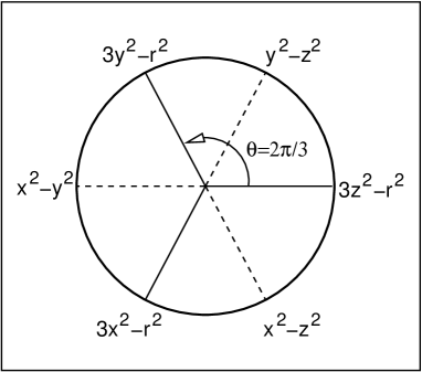
Figure 2: Schematic representation of $e_{g}$ orbitals as obtained for different angle $\theta$ in Eq. (31). Pairs of orthogonal orbitals, forming a basis in the orbital space, differ by angle $\theta=\pi$. Directional $e_{g}$ orbitals $|\zeta\rangle$ along $a$ and $b$ axes are obtained from the $\{|3z^{2}-r^{2}\rangle,|x^{2}-y^{2}\rangle\}$ basis (32) by the transformation (31) with angle $\theta=\pm 2\pi/3$. Dashed lines for $\theta=\pm\pi/3$ indicate the possible OO of $|y^{2}-z^{2}\rangle/|x^{2}-z^{2}\rangle$ orbitals occupied by holes in KCuF₃, suggested for $T<T_{N}$ in Ref. Kug82, .

The magnetic superexchange constants $J_{ab}$ and $J_{c}$ in the effective spin model (11) are obtained by decoupling spin and orbital variables and next averaging the orbital operators in the spin-orbital model (17) over the classical state $|\Phi_{0}\rangle$ as given by Eq. (30). The relevant averages are given in Table 2, and they lead to compact expressions for the superexchange constants in Eq. (11),

$$J_{c} = \frac{1}{8}J\Big{\{}-r_{1}\sin^{2}\theta+(r_{2}+r_{3})(1+\cos\theta)$$ (34)

$$\hskip 14.22636pt+(r_{4}+2R)(1+\cos\theta)^{2}\Big{\}},$$

$$J_{ab} = \frac{1}{8}J\Big{\{}-r_{1}\Big{(}\frac{3}{4}+\sin^{2}\theta\Big{)}+(r_{2}+r_{3})\Big{(}1-\frac{1}{2}\cos\theta\Big{)}$$ (35)

$$\hskip 14.22636pt+(r_{4}+2R)\Big{(}\frac{1}{2}-\cos\theta\Big{)}^{2}\Big{\}},$$

which depend on three parameters, viz. $J$ (7), $\eta$ (19) and $R$ (29), and on the OO (III.2) specified by the orbital angle $\theta$. It is clear that the FM term $\propto r_{1}$ competes with all the other AF low-spin terms. Nevertheless, in the $ab$ planes, where the occupied $e_{g}$ orbitals alternate, the large FM contribution (when $\sin^{2}\theta\sim 1$) still makes the magnetic superexchange $J_{ab}$ weakly FM ($J_{ab}\lesssim 0$), while the stronger AF superexchange along the $c$ axis ($J_{c}\gg|J_{ab}|$) favors quasi one-dimensional (1D) spin fluctuations.

Table 2: Averages of the orbital projection operators standing in the spin-orbital interactions in Eqs. (20)–(23) for the $C$-type (or $G$-type) OO of occupied $e_{g}$ orbitals which alternate in $ab$ planes, as given by Eqs. (III.2). Nonequivalent cubic directions are labelled by $\gamma=ab,c$.

$\gamma$	$ab$	$c$
$\big{\langle}\big{(}\frac{1}{2}-\tau_{i}^{(\gamma)}\big{)}\big{(}\frac{1}{2}-\tau_{j}^{(\gamma)}\big{)}\big{\rangle}$	$\frac{1}{4}\big{(}\frac{1}{2}-\cos\theta\big{)}^{2}$	$\frac{1}{4}\big{(}1+\cos\theta\big{)}^{2}$
$\big{\langle}\frac{1}{4}-\tau_{i}^{(\gamma)}\tau_{j}^{(\gamma)}\big{\rangle}$	$\frac{1}{4}\big{(}\frac{3}{4}+\sin^{2}\theta\big{)}$	$\frac{1}{4}\sin^{2}\theta$
$\big{\langle}\big{(}\frac{1}{2}+\tau_{i}^{(\gamma)}\big{)}\big{(}\frac{1}{2}+\tau_{j}^{(\gamma)}\big{)}\big{\rangle}$	$\frac{1}{4}\big{(}\frac{1}{2}+\cos\theta\big{)}^{2}$	$\frac{1}{4}\big{(}1-\cos\theta\big{)}^{2}$

By considering the superexchange model, one can derive as well the pure orbital interactions which stabilize the OO. The superexchange interactions are anisotropic below the structural transition at $T_{s}$. In contrast, at sufficiently high temperature $T>T_{s}$, when also spin correlations may be neglected, one finds isotropic orbital interactions,

$$J_{c}^{\tau}=J_{ab}^{\rm orb}=\frac{1}{8}J\big{(}3r_{1}-r_{4}-2R\big{)},$$ (36)

which multiply $\tau_{i}^{(\gamma)}\tau_{j}^{(\gamma)}$ for each bond, contributing to an orbital instability towards alternating $G$-type OO, while actually $C$-type OO is observed below $T_{s}$. It is thus clear from experiment that this instability cannot be of purely electronic origin, and that, similarly to what is the case in LaMnO₃, Mil96 it is supported by the lattice. In fact, although it has been argued that the OO is caused primarily by the superexchange, Lic95 the electronic interactions (36) predict that $T_{s}\sim 0.1J$, and not $T_{s}\sim J$, as observed. Note also that as soon as the AF spin correlations develop along the $c$ axis, one finds anisotropic orbital interactions, $J_{ab}^{\tau}>J_{c}^{\tau}$, which amplifies the ongoing symmetry breaking in the tetragonal phase.

The spectral weights of the optical subbands also follow from the superexchange processes, and are determined from the effective Hamiltonian (17) by the general relations given by Eqs. (13) and (15). Following the excitation spectrum of Fig. 1, one finds optical absorption at three different energies (the degeneracy of the ${}^{1}E$ state is not removed), so we label the respective kinetic energy contributions $K_{n}^{(\gamma)}$ by $n=1,2,3$. They are determined at low temperature $T\lesssim 500$ K by rigid $C$-type OO (III.2), with the classical averages of the orbital operators given in Table 2. So one finds for polarization along the $c$ axis

$$K_{1}^{(c)} = \frac{1}{4}Jr_{1}\Big{(}\frac{3}{4}+s_{c}\Big{)}\sin^{2}\theta,$$ (37)

$$K_{2}^{(c)} = \frac{1}{4}J(r_{2}+r_{3})\Big{(}\frac{1}{4}-s_{c}\Big{)}(1+\cos\theta),$$ (38)

$$K_{3}^{(c)} = \frac{1}{4}Jr_{4}\Big{(}\frac{1}{4}-s_{c}\Big{)}(1+\cos\theta)^{2},$$ (39)

and for polarization in the $ab$ plane

$$\!\!K_{1}^{(ab)} \!=\! \frac{1}{4}Jr_{1}\Big{(}\frac{3}{4}+s_{ab})\Big{(}\frac{3}{4}+\sin^{2}\theta\Big{)},$$ (40)

$$\!\!K_{2}^{(ab)} \!=\! \frac{1}{4}J(r_{2}\!+\!r_{3})\Big{(}\frac{1}{4}-\!s_{ab}\Big{)}\Big{(}1\!-\frac{1}{2}\cos\theta\Big{)},$$ (41)

$$\!\!K_{3}^{(ab)} \!=\! \frac{1}{4}Jr_{4}\Big{(}\frac{1}{4}-s_{ab}\Big{)}\Big{(}\frac{1}{2}-\cos\theta\Big{)}^{2}.$$ (42)

Similar to the exchange constants $J_{ab}$ and $J_{c}$, the kinetic energies depend on the multiplet structure described by two parameters, viz. $J$ (7), $\eta$ (19), and on the OO (III.2) specified by the angle $\theta$. Note that they depend on these parameters also indirectly, since the spin-spin correlations are governed by $J_{ab}$ and $J_{c}$ as well. We analyze this dependence in Sec. III.4.

III.3 Magnetic interactions in KCuF₃

In order to apply the above classical theory to KCuF₃ we need to determine the microscopic parameters which decide about the superexchange constants, given by Eqs. (34) and (35). In principle, if the optical data would also be available, with this experimental input one would be able to fix the values of the relevant parameters $J$ and $\eta$, and the orbital angle $\theta$. Having only magnetic measurements, we give here an example of another approach which starts from the microscopic parameters for the local Coulomb interaction and Hund’s element suggested by the electronic structure calculations performed within the LDA+U method:Lic95 ; Med02 $U=7.5$, $J_{H}=0.9$ eV — they lead to $\eta=0.12$. Note that these parameters are somewhat smaller than the values $U=8.96$ and $J_{H}=1.19$ eV deduced for Cu²⁺ ions in the CuO₂ planes of the high-temperature superconductors by Grant and McMahan using the fixed charge method,Gra92 but we believe that they reflect better the partly screened interactions within CuF₆ units. We are not aware of any estimation of the remaining microscopic parameters until now, but taking into account the expected contraction of the $2p$ wavefunctions by going from O^2- to F^- ions, we argue that $t_{pd}$ is reduced, while $\Delta$ and $U_{p}$ could be similar to their respective values for CuO₂ planes.Gra92 Therefore, it is reasonable to adopt: $t_{pd}=1.0$, $\Delta=4.0$, and $U_{p}=4.5$ eV. Note that although the values of $t_{pd}=1.0$, $\Delta$ and $U_{p}$ could not be really estimated, in the present approach they are not independent parameters; also only a linear combination of $\Delta$ and $U_{p}$ enters Eq. (29), so a change in the value of $U_{p}$ could to some extent compensate a modified value of $\Delta$. The present parameters lead to $J\simeq 33.3$ meV and $R=1.2$.

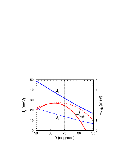
Figure 3: (Color online) Exchange interactions (34): $J_{c}$ (34) and $J_{ab}$ (35) for the copper fluoride model as functions of the orbital angle $\theta$ which describes the OO [see Eq. (30)]. The dashed lines show the $U$ term alone, while the solid lines include the CT contributions as well. The OO induced by the JT distortions ($\theta\simeq 70^{\circ}$) is indicated by dotted line. Parameters: $J\simeq 33.3$ meV, $\eta=0.12$, $R=1.2$.

Consider now the OO of the occupied orbitals (by holes) in KCuF₃. Recent resonant x-ray scattering experiments suggest that both sublattices are equivalent, with $\theta_{A}=-\theta_{B}=\theta$ in Eq. (30),Pao02 but the precise shape of the occupied orbitals in KCuF₃ remains unresolved. There are different views concerning the type of orbitals that participate in the OO state. On the one hand, it is believed that the orbital angle $\theta$ should be close to the angle $\theta_{\rm JT}\simeq 70^{\circ}$ ($\sim 0.39\pi$), as given by $\cos\theta\simeq\frac{1}{3}$, which follows from the local lattice distortions.Kad67 On the other hand, the electronic interactions in the symmetry broken $A$-AF phase below $T_{N}$ would favor instead alternating $(y^{2}-z^{2})/(x^{2}-z^{2})$ orbitals,Kug82 with $\theta_{\rm SE}=60^{\circ}$. In reality, one expects rather a certain compromise between the electronic interactions for finite spin correlations and those induced by the lattice. Thus, in the present study of the magnetic exchange constants and optical spectral weights we shall consider a range of possible values of $60^{\circ}<\theta<90^{\circ}$, focusing in particular on the above values favored by the above individual terms in the effective Hamiltonian.

First, we demonstrate that the model Eq. (17) is capable of describing the experimentally observed exchange constants $J_{c}^{\rm exp}\simeq 35$ meV and $J_{ab}^{\rm exp}\simeq-2$ meV. Ten93 Remarkably, the value of $|J_{ab}^{\rm exp}|$ is smaller by more than one order of magnitude than $J_{c}^{\rm exp}$, being some challenge for the theoretical model. Consider first the values of $J_{c}$ and $J_{ab}$ for varying angle $\theta$ which tunes the OO (Fig. 3). When only the $U$ part of the superexchange ${\cal H}_{U}$ is considered, one finds $J_{c}\sim 15$ meV and $J_{ab}\sim-2$ meV. The FM term $\propto r_{1}$ gives the largest contribution for the $ab$ planes, which follows from the alternation of hole orbitals in the $ab$ planes, being close to the planar orbitals $(x^{2}-z^{2})/(y^{2}-z^{2})$ ($\theta=60^{\circ}$) suggested early on by Kugel and Khomskii, Kug82 but is partly compensated by the AF terms. While $J_{ab}$ is only weakly depending on $\theta$ near this type of OO, $J_{c}$ decreases steadily with increasing $\theta$ (Fig. 3), as the overlap between the orbitals occupied by holes along the $c$ axis decreases when the amplitude of the $|z\rangle$ states is reduced. One finds that using only the $U$ term in the superexchange, rather extreme parameters, such as $U<4$ eV and $J_{H}\sim 0.3$ eV (with the present value of $t$), would have to be assumed to reproduce the experimental values of $J_{c}$ and $J_{ab}$.

The CT term (III.1) with $R=1.2$ enhances the AF interaction $J_{c}$ by a factor larger than two but hardly changes $J_{ab}$ (see Fig. 3). Only then $J_{c}$ comes close to the experimental value $J_{c}^{\rm exp}\simeq 35$ meV.Ten93 As in the $U$ model (at $R=0$), the value of $J_{c}$ decreases with increasing $\theta$, and there is no serious difficulty to fit the parameters in order to obtain a reasonable agreement with experiment, once the value of the orbital angle $\theta$ would be known. As an illustrative example we show the results obtained with the present parameters in Fig. 3 — one finds $J_{c}\simeq 32$ meV for the OO which agrees with the lattice distortions ($\theta_{\rm JT}\simeq 70^{\circ}$), and $J_{c}\simeq 40$ meV for the Kugel-Khomskii $(x^{2}-z^{2})/(y^{2}-z^{2})$ orbitals ($\theta_{\rm SE}=60^{\circ}$). These results demonstrate that the CT superexchange term plays an essential role in KCuF₃ and so this system has to be classified as a charge transfer insulator.

Remarkably, the value of $J_{ab}$ is almost unaffected by the CT term (Fig. 3). This is due to the alternating OO in the $ab$ planes, which makes the value of the orbital projection $\big{\langle}\big{(}\frac{1}{2}-\tau_{i}^{(\gamma)}\big{)}\big{(}\frac{1}{2}-\tau_{j}^{(\gamma)}\big{)}\big{\rangle}$ in Eq. (III.1) very small indeed in the physical range of $\theta$ (compare Table 2). In fact, for the alternating planar $(x^{2}-z^{2})/(y^{2}-z^{2})$ orbitals one of the operators $\{\big{(}\frac{1}{2}-\tau_{i}^{(\gamma)}\big{)},\big{(}\frac{1}{2}-\tau_{j}^{(\gamma)}\big{)}\}$ equals zero, and the CT contribution vanishes, so one cannot reduce the value of $|J_{ab}|$ by increasing the AF CT term that follows from ${\cal H}_{\Delta}$.

Figure 4: Ratio of the exchange interactions $|J_{ab}|/J_{c}$ in KCuF₃, given by Eqs. (34) and (35), for increasing charge transfer parameter $R$, obtained for a few values of $\eta$ and for the OO induced by the JT effect ($\theta\simeq 70^{\circ}$, solid lines). The dashed line shows $|J_{ab}|/J_{c}$ obtained for $\eta=0.12$ and for alternating $(x^{2}-z^{2})/(y^{2}-z^{2})$ orbitals ($\theta=60^{\circ}$).

The strong anisotropy of the magnetic exchange interactions in KCuF₃ is well illustrated in Fig. 4 by the ratio $|J_{ab}|/J_{c}$, being close to 0.07 for either the JT OO ($\theta\simeq 70^{\circ}$), or for the OO suggested by the orbital superexchange at $T<T_{N}$ ($\theta=60^{\circ}$). Note that for $R\sim 1$ the ratio $|J_{ab}|/J_{c}$ does not depend significantly on $\theta$ in the interesting range between $\theta=70^{\circ}$ and $\theta=60^{\circ}$.

III.4 Optical spectral weights for KCuF₃

Now we turn to the optical spectral weights (13) and determine the kinetic energies for the corresponding Hubbard subbands. As discussed in Sec. II, they originate from different multiplet excitations, and depend on the OO and on the spin-spin correlations (12). Here we analyze in detail the spectral weight distribution for polarization along the $c$ axis, where strong exchange interaction $J_{c}$ controls the spin-spin correlations $s_{c}$ (12) which remain finite in a broad temperature regime.

Knowing that the interchain FM exchange coupling $J_{ab}$ is so weak, we describe the temperature variation of the spin-spin correlations $s_{c}=\langle\vec{S}_{i}\!\cdot\!\vec{S}_{i+1}\rangle_{c}$ employing the Jordan-Wigner fermion representationMat85 for a 1D spin chain. One finds for perfect OO at temperature $T<T_{s}$

$$s_{c}=-\kappa(1+\kappa),$$ (43)

where

$$\kappa = \frac{1}{N}\,\sum_{k}\;|\cos k|\,\tanh\Big{(}\frac{\varepsilon_{k}}{2k_{B}T}\Big{)},$$ (44)

$$\varepsilon_{k} = J_{c}(1+2\kappa)|\cos k|.$$ (45)

Here $\varepsilon_{k}$ is the 1D dispersion of pseudofermions. The exchange interaction $J_{c}$ is constant as long as the orbitals remain frozen, and sets the energy scale for the temperature variation of $s_{c}$. Eqs. (44) and (45) were solved self-consistently to obtain $s_{c}$ (43) as a function of temperature. In the limit $T\to 0$ one finds $\kappa=1/\pi$, and $s_{c}=-(1+\pi)/\pi^{2}\simeq 0.42$. This value represents an excellent analytic approximation to the exact result,

$$s_{c}^{\rm ex}=-(\log 2-\textstyle{\frac{1}{4}})\simeq-0.4431,$$ (46)

obtained for the 1D AF Heisenberg chain from the Bethe ansatz. Mat85

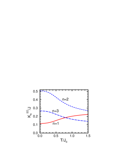
Figure 5: (Color online) Kinetic energy terms per bond (13), as obtained for the $c$ axis with the OO (30) suggested by the JT distortions ($\theta\simeq 70^{\circ}$) in KCuF₃ (in units of $J$): high-spin $K_{1}^{(c)}$ (solid line) and low-spin $K_{2,3}^{(c)}$ (dashed lines), for increasing temperature $T/J_{c}$. Parameters as in Fig. 3.

Table 3: Kinetic energies of the different Hubbard subbands ($K_{n}^{(\gamma)}$), and total kinetic energies ($K^{(\gamma)}$) (in meV), as obtained for KCuF₃ for two representative orbital states: $\theta_{\rm JT}\simeq 70^{\circ}$ and $\theta_{\rm SE}=60^{\circ}$. Parameters: $J\simeq 33.3$ meV, $\eta=0.12$.

	$\theta_{\rm JT}\simeq 70^{\circ}$				$\theta_{\rm SE}=60^{\circ}$
	$T=0$	$40$ K	$300$ K		$T=0$	$40$ K	$300$ K
$K_{1}^{(c)}$	3.8	3.9	6.1		3.2	3.3	5.2
$K_{2}^{(c)}$	16.9	16.8	11.9		19.0	18.9	13.4
$K_{3}^{(c)}$	8.9	8.8	6.2		11.2	11.1	7.9
$K^{(c)}$	29.6	29.5	24.2		33.4	33.3	26.5
$K_{1}^{(ab)}$	21.3	16.0	16.0		19.5	14.6	14.6
$K_{2}^{(ab)}$	0.0	3.9	3.9		0.0	3.6	3.6
$K_{3}^{(ab)}$	0.0	0.1	0.1		0.0	0.0	0.0
$K^{(ab)}$	21.3	20.0	20.0		19.5	18.2	18.2

The general theory presented in Sec. II makes a clear prediction concerning the temperature dependence of the spectral weights in optical absorption. First of all, a large anisotropy between the polarization along the AF $c$ axis and the polarization in the (weakly FM) $ab$ plane is expected when the AF (FM) spin-spin correlations along the $c$ axis (within the $ab$ planes) develop. Indeed, using the self-consistent solution of Eqs. (44) and (45), one finds that the kinetic energy $K_{1}^{(c)}$ (which determines the spectral weight of the high-spin excitation at energy $U-3J_{H}$) is rather low (Fig. 5). In contrast, the low-spin excitations $K_{2}^{(c)}$ and $K_{3}^{(c)}$ contribute with large spectral weights in the low temperature regime, reflecting the AF correlations along the $c$ axis.

When the temperature increases, the spin-spin correlations $s_{c}$ gradually weaken and the kinetic energy redistributes — both low-spin terms $K_{2}^{(c)}$ and $K_{3}^{(c)}$ decrease, while the high-spin term $K_{1}^{(c)}$ increases as more high-spin excitations are then allowed (Fig. 5). For the considered OO given by $\theta_{JT}\simeq 70^{\circ}$, the changes of the contributions at the two lower energies which correspond to $n=1$ and $n=2$ are particularly large between zero and room temperature (up to $k_{B}T/J_{c}\simeq 0.8$), with the increase (decrease) of $K_{1}^{(c)}$ [$K_{2}^{(c)}$] by $\sim 60$ ($\sim 33$) percent of the reference value at $T=0$. This leads to rather similar values of all three contributions at room temperature. This predicted behavior could be verified by future experiments.

The temperature variation of the spectral weights for $ab$ polarization is more difficult to predict as it involves weak $s_{ab}$ spin correlations which develop in the temperature range $T\sim T_{N}$, and grow with increasing order parameter, $s_{ab}\propto|\langle S^{z}\rangle|$, below $T_{N}$.Sch96 Assuming the classical value for $s_{ab}=0.25$ at $T\to 0$, one finds that the kinetic energy would come entirely from the high-spin optical excitations $K_{1}^{(ab)}$, while the low-spin excitations would be fully suppressed (Table 3). Above $T_{N}$ the spin system is controlled by the dominating AF exchange constant $J_{c}$, and $s_{ab}\simeq 0$. Even then the high-spin excitations at low energy dominate and have large spectral weight as a result of the persisting OO. Some decrease of $K_{1}^{(ab)}$ accompanied by the increase of $K_{1}^{(c)}$ with increasing temperature makes the anisotropy between $K_{1}^{(c)}$ and $K_{1}^{(ab)}$ considerably less pronounced, but this anisotropy of the spectra in the low energy range remains still close to 3:1 even at room temperature (Table 3). Note also that the highest energy excitation for the $ab$ polarization vanishes at $\theta_{\rm SE}=60^{\circ}$, and gives a negligible contribution for the JT angle $\theta_{\rm JT}\simeq 70^{\circ}$, due to the orbital correlations within the $ab$ planes.

Finally, we would like to emphasize again that knowing only the exchange constants $J_{ab}$ and $J_{c}$ in KCuF₃, one is not able to determine all the microscopic parameters of the CT model. We emphasize that a better understanding of the properties of KCuF₃ can be achieved only by combining the results of magnetic and optical experiments, after the latter experiments have been performed.

IV Cubic manganite: LaMnO₃

IV.1 Superexchange model

Although $e_{g}$ and $t_{2g}$ electrons behave quite differently in LaMnO₃ and are frequently treated as two subsystems, Dag02 ; Dag03 the neutron experimentsMou96 which measure the spin waves in the $A$-AF phase below $T_{N}$ leave no doubt that an adequate description of the magnetic properties requires a magnetic Hamiltonian of the form given by Eq. (11), describing superexchange between total $S=2$ spins of the Mn³⁺ ions. The high-spin ${}^{5}E$ ground state at each Mn³⁺ ion is stabilized by the large Hund’s exchange $J_{H}$. The situation is here more complex than either in KCuF₃ (Sec. III) or in the $t_{2g}$ systems discussed in the following Sections, however, as the superexchange terms between Mn³⁺ ions originate from various charge excitations $d_{i}^{4}d_{j}^{4}\rightleftharpoons d_{i}^{5}d_{j}^{3}$, made either by $e_{g}$ or by $t_{2g}$ electrons, leading to different excited states in the intermediate $d^{5}$ configuration on a Mn${}^{2+}(d_{i}^{5})$ ion. Such processes determine the $U$ term ${\cal H}_{U}(d^{4})$ defined by Eq. (6), and were analyzed in detail in Ref. Fei99, , and lead to the structure of ${\cal H}_{U}(d^{4})$ given below. However, the CT processes, ${\cal H}_{\Delta}(d^{4})$, contribute as well and the complete model for LaMnO₃ reads

$${\cal H}(d^{4})={\cal H}_{U}(d^{4})+{\cal H}_{\Delta}(d^{4}).$$ (47)

The superexchange constant $J$ is here defined again by Eq. (7), using an average hopping element along an effective $(dd\sigma)$ bond, $t=t_{pd}^{2}/\bar{\Delta}$, where $\bar{\Delta}$ is an average CT excitation energy, introduced below in Eq. (65).

First we analyze the structure of the $U$ term for LaMnO₃, ${\cal H}_{U}(d^{4})$, due to excitations involving $e_{g}$ electrons. The energies of the five possible excited states:Gri71 (i) the high-spin ${}^{6}\!A_{1}$ state($S=5/2$), and (ii-v) the low-spin ($S=3/2$) states: ${}^{4}\!A_{1}$, ${}^{4}E$ (${}^{4}E_{\epsilon}$, ${}^{4}E_{\theta}$), and ${}^{4}\!A_{2}$, will be parametrized again by the intraorbital Coulomb element $U$ (3), and by Hund’s exchange $J_{H}$ between a pair of $e_{g}$ electrons, defined in Eq. (18). notejh The energies of the excited states are given in terms of the Racah parameters in Ref. Gri71, ; in order to parametrize this spectrum by $J_{H}$ we apply an approximate relation $4B\simeq C$ which holds for the spectroscopic values of the Racah parameters for a Mn²⁺ ($d^{5}$) ion:Zaa90 ; Boc92 $B=0.107$ eV and $C=0.477$ eV. Here we use these atomic values as an example of the theory — using them and Eq. (18) one finds the excitation spectrum: $U-3J_{H}$, $U+3J_{H}/4$, $U+5J_{H}/4$, $U+5J_{H}/4$, and $U+13J_{H}/4$ [Fig. 1(a)]. Unlike $J_{H}$, the value of $U$ is known with less accuracy — hence we shall use it here only as a parameter which can be deduced a posteriori from the superexchange $J$ which is able to explain the experimental values for two exchange constants responsible for the $A$-AF phase observed in LaMnO₃ well below the structural transition (here again $T_{N}\ll T_{s}$).

Using the spin algebra (Clebsch-Gordon coefficients), and making a rotation of the terms derived for a bond $\langle ij\rangle\parallel c$ to the other two cubic axes $a$ and $b$, one finds five contributions to ${\cal H}_{U}(d^{4})$ due to different $(t_{2g}^{3}e_{g}^{1})_{i}(t_{2g}^{3}e_{g}^{1})_{j}\rightleftharpoons(t_{2g}^{3}e_{g}^{2})_{i}(t_{2g}^{3})_{j}$ excitations by $e_{g}$ electrons,Fei99

$$\!H_{1}^{(\gamma)}\! = \!-\frac{J}{20}r_{1}\big{(}\vec{S}_{i}\!\cdot\!\vec{S}_{j}+6\big{)}\Big{(}\frac{1}{4}-\tau_{i}^{(\gamma)}\tau_{j}^{(\gamma)}\Big{)},$$ (48)

$$\!H_{2}^{(\gamma)}\! = \!\!\frac{3J}{160}r_{2}\big{(}\vec{S}_{i}\!\cdot\!\vec{S}_{j}-4\big{)}\Big{(}\frac{1}{4}-\tau_{i}^{(\gamma)}\tau_{j}^{(\gamma)}\Big{)},$$ (49)

$$\!H_{3}^{(\gamma)}\! = \!\!\frac{J}{32}r_{3}\big{(}\vec{S}_{i}\!\cdot\!\vec{S}_{j}-4\big{)}\Big{(}\frac{1}{4}-\tau_{i}^{(\gamma)}\tau_{j}^{(\gamma)}\Big{)},$$ (50)

$$\!H_{4}^{(\gamma)}\! = \!\!\frac{J}{32}r_{4}\big{(}\vec{S}_{i}\!\cdot\!\vec{S}_{j}-4\big{)}\!\Big{(}\frac{1}{2}-\!\tau_{i}^{(\gamma)}\Big{)}\!\Big{(}\frac{1}{2}-\!\tau_{j}^{(\gamma)}\Big{)},$$ (51)

$$\!H_{5}^{(\gamma)}\! = \!\!\frac{J}{32}r_{5}\big{(}\vec{S}_{i}\!\cdot\!\vec{S}_{j}-4\big{)}\!\Big{(}\frac{1}{2}-\!\tau_{i}^{(\gamma)}\Big{)}\!\Big{(}\frac{1}{2}-\!\tau_{j}^{(\gamma)}\Big{)},$$ (52)

where the coefficients

$$r_{1} = \frac{1}{1-3\eta},\hskip 42.67912ptr_{2}=\frac{1}{1+3\eta/4},$$

$$r_{3} = r_{4}=\frac{1}{1+5\eta/4},\hskip 8.5359ptr_{5}=\frac{1}{1+13\eta/4},$$ (53)

follow from the above multiplet structure of Mn²⁺ ($d^{5}$) ions, and $\eta$ (19) stands for the Hund’s exchange. The meaning of the various terms is straightforward: the first term $H_{1}^{(\gamma)}$ describes the high-spin excitations to the ${}^{6}\!A_{1}$ state while the remaining ones, $H_{n}^{(\gamma)}$ with $n=2,\dots,5$, arise due to the low-spin excited states ${}^{4}\!A_{1}$, ${}^{4}E_{\theta}$, ${}^{4}E_{\epsilon}$ and ${}^{4}\!A_{2}$, respectively. The orbital dependence is given by the same operators (27) as in Sec. III. Similar to the case of the ${}^{1}E$ state for the copper fluoride [see Eqs. (21) and (22)], the doubly degenerate ${}^{4}E$ state contributes here with two terms characterized by a different orbital dependence in Eqs. (50) and (51). Note that this degeneracy would be removed by the cooperative JT effect, i.e., the structural phase transition (and associated OO) driven by the local JT coupling in combination with the elastic lattice forces. The resulting small level splitting we neglect here, and so we set $r_{3}=r_{4}$.

The superexchange mediated by $t_{2g}$ electrons results from $(t_{2g}^{3}e_{g}^{1})_{i}(t_{2g}^{3}e_{g}^{1})_{j}\rightleftharpoons(t_{2g}^{4}e_{g}^{1})_{i}(t_{2g}^{2}e_{g}^{1})_{j}$ excitations which involve ${}^{4}T_{1}$ and ${}^{4}T_{2}$ configurations at both Mn ions: Mn²⁺ and Mn⁴⁺. They give low $S=3/2$ spins of Mn²⁺ ions, and this part of the superexchange is AF. Using the present units introduced in Eqs. (3) and (18), one finds the excitation energies (not shown in Fig. 1): $\varepsilon(^{4}T_{1},^{4}T_{2})\simeq U+5J_{H}/4$, $\varepsilon(^{4}T_{2},^{4}T_{2})\simeq U+9J_{H}/4$, $\varepsilon(^{4}T_{1},^{4}T_{1})\simeq U+11J_{H}/4$, and $\varepsilon(^{4}T_{2},^{4}T_{1})\simeq U+15J_{H}/4$, with the first (second) label standing for the configuration of the Mn²⁺ (Mn⁴⁺) ion, respectively. In the actual derivation each of the excited states, with one $t_{2g}$ orbital being either doubly occupied or empty, has to be projected on the respective eigenstates and the spin algebra is next used to construct the interacting total $S=2$ spin states. This leads to the final contribution to ${\cal H}_{U}$ which, in a good approximation, is orbital independent,Fei99

$$H_{6}^{(\gamma)}=\frac{1}{8}J\beta r_{t}\Big{(}\vec{S}_{i}\!\cdot\!\vec{S}_{j}-4\Big{)}.$$ (54)

Here $\beta=(t_{\pi}/t)^{2}$ follows from the difference between the effective $d-d$ hopping elements along the $\sigma$ and $\pi$ bonds, and we adopt the Slater-Koster value $\beta=1/9$. The coefficient $r_{t}$ stands for a superposition of the above $t_{2g}$ excitations involved in the $t_{2g}$ superexchange,

$$r_{t}=\frac{1}{4}\Big{(}\frac{1}{1+\textstyle{\frac{5}{4}}\eta}+\frac{1}{1+\textstyle{\frac{9}{4}}\eta}+\frac{1}{1+\textstyle{\frac{11}{4}}\eta}+\frac{1}{1+\textstyle{\frac{15}{4}}\eta}\Big{)}.$$ (55)

There is no need to distinguish between the different excitation energies; all of them are significantly higher than the first low-spin excitation energy for the configuration ${}^{4}\!A_{1}$, which occurs after an excitation by an $e_{g}$ electron.

While earlier studies of the superexchange interactions in manganites were limited to model Hamiltonians containing only the $U$ term, Dag02 ; Ish97 ; Fei99 ; Feh04 the importance of the CT processes was emphasized only recently.Mes01 For our purposes we derived the CT term ${\cal H}_{\Delta}(d^{4})$ by considering again excitations by either $\sigma$ or $\pi$ electrons on the bond $\langle ij\rangle$, leading to two-hole excited states at an intermediate oxygen, $d^{4}_{i}(2p_{\langle ij\rangle})^{6}d^{4}_{j}\rightleftharpoons d^{5}_{i}(2p_{\langle ij\rangle})^{4}d^{5}_{j}$. Unlike in KCuF₃ with a unique CT excitation, however, in the present case a number of different excited states occurs with the excitation energies depending on the electronic configuration of the two intermediate Mn²⁺ ions at sites $i$ and $j$. One finds that these various excitations can be parametrized by a single parameter $R$ given by Eq. (29), and the excited states on two neighboring transition metal ions contribute, as for the $U$ term, both FM and AF terms,

$$H_{\Delta}(d^{4}) = \frac{1}{16}JR\sum_{\langle ij\rangle\parallel\gamma}\Big{\{}c_{1}\Big{(}\vec{S}_{i}\cdot\vec{S}_{j}-4\Big{)}\Big{(}\frac{1}{2}-\tau_{i}^{(\gamma)}\Big{)}\Big{(}\frac{1}{2}-\tau_{j}^{(\gamma)}\Big{)}$$ (56)

$$+ \frac{8}{5}\Big{[}-c_{2}\Big{(}\vec{S}_{i}\cdot\vec{S}_{j}+6\Big{)}+c_{3}\Big{(}\vec{S}_{i}\cdot\vec{S}_{j}-4\Big{)}\Big{]}\Big{(}\frac{1}{4}-\tau_{i}^{(\gamma)}\tau_{j}^{(\gamma)}\Big{)}$$

$$+ \frac{8}{5}\Big{[}-c_{4}\Big{(}\vec{S}_{i}\cdot\vec{S}_{j}+6\Big{)}+c_{5}\Big{(}\vec{S}_{i}\cdot\vec{S}_{j}-4\Big{)}\Big{]}\Big{(}\frac{1}{2}+\tau_{i}^{(\gamma)}\Big{)}\Big{(}\frac{1}{2}+\tau_{j}^{(\gamma)}\Big{)}\Big{\}}$$

$$+ \frac{1}{8}JR\beta c_{t}\sum_{\langle ij\rangle}\Big{(}\vec{S}_{i}\cdot\vec{S}_{j}-4\Big{)},$$

where the coefficients $c_{n}$, with $n=1,\cdots,5$, and $c_{t}$ are all determined by $\eta$ and $R$ via $\eta^{\prime}=\eta R$:

$$c_{1} = \frac{1}{4}\Big{(}\frac{1}{1+\textstyle{\frac{17}{4}}\eta^{\prime}}+\frac{2}{1+\textstyle{\frac{21}{4}}\eta^{\prime}}+\frac{1}{1+\textstyle{\frac{25}{4}}\eta^{\prime}}\Big{)},$$ (57)

$$c_{2} = \frac{1}{2}\Big{(}\frac{1}{1+\textstyle{\frac{17}{8}}\eta^{\prime}}+\frac{1}{1+\textstyle{\frac{25}{8}}\eta^{\prime}}\Big{)},$$ (58)

$$c_{3} = \frac{1}{16}\Big{(}\frac{3}{1+4\eta^{\prime}}+\frac{5}{1+\textstyle{\frac{17}{4}}\eta^{\prime}}+\frac{3}{1+5\eta^{\prime}}+\frac{5}{1+\textstyle{\frac{21}{4}}\eta^{\prime}}\Big{)},$$ (59)

$$c_{4} = \frac{1}{5}+\frac{1}{10}\Big{(}\frac{3}{1+\textstyle{\frac{15}{8}}\eta^{\prime}}+\frac{5}{1+\textstyle{\frac{17}{8}}\eta^{\prime}}\Big{)},$$ (60)

$$c_{5} = \frac{3}{5}+\frac{1}{160}\Big{(}\frac{9}{1+\textstyle{\frac{15}{4}}\eta^{\prime}}+\frac{30}{1+4\eta^{\prime}}+\frac{25}{1+\textstyle{\frac{17}{4}}\eta^{\prime}}\Big{)},$$ (61)

$$c_{t} = \frac{1}{4}\Big{(}\frac{1}{1+\textstyle{\frac{17}{4}}\eta^{\prime}}+\frac{2}{1+\textstyle{\frac{19}{4}}\eta^{\prime}}+\frac{1}{1+\textstyle{\frac{21}{4}}\eta^{\prime}}\Big{)}.$$ (62)

The coefficients $c_{n}$ follow from CT excitations by $e_{g}$ electrons. As in the copper fluoride case (Sec. III), the lowest (high-spin) excitation energy will be labeled by $\Delta$,

$$\Delta(^{6}\!A_{1})=\Delta,$$ (63)

so the other possible individual (low-spin) excitations at each transition metal ion have the energies

$$\Delta(^{4}\!A_{1}) = \Delta+\frac{15}{4}J_{H},$$

$$\Delta(^{4}E) = \Delta+\frac{17}{4}J_{H},$$

$$\Delta(^{4}\!A_{2}) = \Delta+\frac{25}{4}J_{H},$$ (64)

These excitation energies are used here to introduce an average CT energy $\bar{\Delta}$,

$$\frac{1}{\bar{\Delta}}=\frac{1}{26}\Big{(}\frac{8}{\Delta(^{6}\!A_{1})}+\frac{3}{\Delta(^{4}\!A_{1})}+\frac{10}{\Delta(^{4}E)}+\frac{5}{\Delta(^{4}\!A_{2})}\Big{)},$$ (65)

which serves to define the effective hopping element $t=t_{pd}^{2}/\bar{\Delta}$, and the superexchange energy $J$ (7) in a microscopic approach. We emphasize, however, that such microscopic parameters as $\{t_{pd},\bar{\Delta},U,J_{H}\}$ will not be needed here, and only the values of the effective parameters $\{J,\eta,R\}$ will decide about the exchange constants and the optical spectral weights.

Each coefficient $c_{n}$ (57), with $n=1,\cdots,5$, stands for an individual process which contributes with a particular orbital dependence due to an intermediate state arising in the excitation process, and accompanies either a FM or an AF spin factor, depending on whether high-spin or low-spin states are involved. As in the $U$ term (48)–(54), a pair of directional $|\zeta\rangle$ orbitals accompanies low-spin excitations, while either high-spin or low-spin excited states are allowed when two different orbitals, one directional and one orthogonal to it (planar orbital), are occupied at the two Mn³⁺ sites. In contrast to the $U$ term, also configurations with two planar orbitals $|\xi\rangle$ occupied at sites $i$ and $j$ contribute to ${\cal H}_{\Delta}(d^{4})$ in Eq. (56). These terms are accompanied by the projection operator $\big{\langle}(\frac{1}{2}+\tau_{i}^{(\gamma)})(\frac{1}{2}+\tau_{j}^{(\gamma)})\big{\rangle}$ in Eq. (56). Note that in the case of the $U$ term such configurations did not contribute as the $e_{g}$ electrons were then blocked and could not generate any superexchange terms. As the electrons from an oxygen $2p_{\sigma}$ orbital are excited instead to directional $|\zeta\rangle$ orbitals at two neighboring Mn³⁺ ions, again both high-spin ($S=5/2$) and low-spin ($S=3/2$) excitations are here possible, giving a still richer structure of ${\cal H}_{\Delta}(d^{4})$.

The OO in LaMnO₃ is robust and sets in below the structural transition at $T_{s}\simeq 780$ K.Mur98 The orbital interactions present in the superexchange Hamiltonian (47) would induce a $G$-type OO.Bri99 The observed classical ground state, which can again be described by Eq. (III.2), corresponds instead to $C$-type OO, as deduced from the lattice distortions. Note that in contrast to KCuF₃, the occupied orbitals refer now to electrons and thus the values of the expected orbital angle $\theta$ are $>90^{\circ}$ (which corresponds to $\cos\theta\lesssim 0$) and so are distinctly different from the copper fluoride case. The averages of the orbital operators in the orbital ordered state are given in Table 2, including the terms $\big{\langle}(\frac{1}{2}+\tau_{i}^{(\gamma)})(\frac{1}{2}+\tau_{j}^{(\gamma)})\big{\rangle}$ which contribute now to the CT part of superexchange. The dependence on the orbital angle $\theta$ suggests that, similar to KCuF₃, these new terms are more significant along the $c$ axis for the OO expected in the manganites.

IV.2 Spin exchange constants and optical intensities

For a better understanding of the effective exchange interactions it is convenient to introduce first the $t_{2g}$ superexchange constant $J_{t}$ which stands for the interaction induced by the charge excitations of $t_{2g}$ electrons. When the CT terms are included, $J_{t}$ consists of the two contributions given in Eqs. (54) and (56),

$$J_{t}=J_{tU}+J_{t\Delta}=\frac{1}{8}J\beta(r_{t}+Rc_{t}).$$ (66)

This interaction is frequently called the superexchange between the core spins. We emphasize that this term is orbital independent and thus isotropic. The coupling constant $J_{t}$ has a similar origin as the $e_{g}$ part of the superexchange $J^{(\gamma)}_{e}$, which however is orbital dependent and anisotropic. We emphasize that both $J_{t}$ and $J^{(\gamma)}_{e}$ are relatively small fractions of $J$.

The $e_{g}$ contributions to the effective exchange constants (11) in LaMnO₃ depend on the orbital state characterized again by Eqs. (III.2) via the averages of the orbital operators,

$$J^{(\gamma)}_{e} = \frac{1}{16}J\Big{\{}-\frac{4}{5}\Big{(}r_{1}-\frac{3}{8}r_{2}-\frac{5}{8}r_{3}\Big{)}\Big{\langle}\frac{1}{4}-\tau_{i}^{(\gamma)}\tau_{j}^{(\gamma)}\Big{\rangle}$$ (67)

$$+ \frac{1}{2}(r_{4}+r_{5})\Big{\langle}\Big{(}\frac{1}{2}-\tau_{i}^{(\gamma)}\Big{)}\Big{(}\frac{1}{2}-\tau_{j}^{(\gamma)}\Big{)}\Big{\rangle}\Big{\}}$$

$$+ \frac{1}{16}JR\Big{\{}c_{1}\Big{\langle}\Big{(}\frac{1}{2}-\tau_{i}^{(\gamma)}\Big{)}\Big{(}\frac{1}{2}-\tau_{j}^{(\gamma)}\Big{)}\Big{\rangle}$$

$$+ \frac{8}{5}(c_{3}-c_{2})\Big{\langle}\frac{1}{4}-\tau_{i}^{(\gamma)}\tau_{j}^{(\gamma)}\Big{\rangle}$$

$$+ \frac{8}{5}(c_{5}-c_{4})\Big{\langle}\Big{(}\frac{1}{2}+\tau_{i}^{(\gamma)}\Big{)}\Big{(}\frac{1}{2}+\tau_{j}^{(\gamma)}\Big{)}\Big{\rangle}\Big{\}}.$$

As the structural transition occurs at relatively high temperature $T_{s}=780$ K, at room temperature (and below it) the OO may be considered to be frozen and specified by an angle $\theta$ [see Eqs. (III.2)]. The orbital fluctuations are then quenched by the combined effect of the orbital part of the $e_{g}$ superexchange in Eqs. (48)-(52) and the orbital interactions induced by the JT effect,Fei99 and the spins effectively decouple from the orbitals, leading to the effective spin model (11). The magnetic transition then takes place within this OO state, and is driven by the magnetic part of the superexchange interactions, which follow from ${\cal H}_{U}(d^{4})$ and ${\cal H}_{\Delta}(d^{4})$. For the $C$-type OO, as observed in LaMnO₃,Mur98 one finds the effective exchange constants in Eq. (11) as a superposition of $J_{t}$ and $J^{(\gamma)}_{e}$ after inserting the averages of the orbital operators (see Table 2) in Eq. (67):

$$J_{ab} = \frac{1}{16}J\Big{\{}-\frac{1}{5}\Big{(}r_{1}-\frac{3}{8}r_{2}\Big{)}\Big{(}\frac{3}{4}+\sin^{2}\theta\Big{)}+\frac{1}{4}r_{3}\Big{(}1-\frac{1}{2}\cos\theta\Big{)}+\frac{1}{8}r_{5}\Big{(}\frac{1}{2}-\cos\theta\Big{)}^{2}\Big{\}}$$ (68)

$$+ \frac{1}{64}JR\Big{\{}c_{1}\Big{(}\frac{1}{2}-\cos\theta\Big{)}^{2}+\frac{8}{5}\big{(}c_{3}-c_{2}\big{)}\Big{(}\frac{3}{4}+\sin^{2}\theta\Big{)}+\frac{8}{5}\big{(}c_{5}-c_{4}\big{)}\Big{(}\frac{1}{2}+\cos\theta\Big{)}^{2}\Big{\}}+J_{t},$$

$$J_{c} = \frac{1}{16}J\Big{\{}-\frac{1}{5}\Big{(}r_{1}-\frac{3}{8}r_{2}\Big{)}\sin^{2}\theta+\frac{1}{4}r_{3}(1+\cos\theta)+\frac{1}{8}r_{5}(1+\cos\theta)^{2}\Big{\}}$$ (69)

$$+ \frac{1}{64}JR\Big{\{}c_{1}(1+\cos\theta)^{2}+\frac{8}{5}\big{(}c_{3}-c_{2}\big{)}\sin^{2}\theta+\frac{8}{5}\big{(}c_{5}-c_{4}\big{)}(1-\cos\theta)^{2}\Big{\}}+J_{t}.$$

Considering $\beta=1/9$ to be fixed by the Slater-Koster parametrization, a complete set of parameters which determines $J_{c}$ and $J_{ab}$ comprises: $J$ (7), $\eta$ (19), $R$ (29), and the orbital angle $\theta$ which defines the phase with OO by Eqs. (III.2), referring now to the orbitals occupied by electrons.

Equations (68) and (69) may be further analyzed in two ways: either (i) using an effective model which includes only the $U$ superexchange term due to $d-d$ transitions, as presented in Ref. Fei99, and discussed in Appendix A (i.e., taking $R=0$ which implies ${\cal H}_{\Delta}(d^{4})\equiv 0$), or (ii) by considering the complete ${\cal H}(d^{4})$ model as given by Eq. (47), which includes also the CT contributions to the superexchange (with $R>0$). By a similar analysis in Sec. III we have established that the CT terms are of essential importance in KCuF₃ and should not be neglected, as otherwise the strong anisotropy of the exchange constants would remain unexplained. Here the situation is qualitatively different — as we show in Appendix A, using somewhat modified parameters $J$ and $\eta$ one may still reproduce the experimental values of the exchange constants, deduced from neutron experiments for LaMnO₃,Mou96 within the effective model at $R=0$, and even interpret successfully the optical spectra.Kov04

It is important to realize that the high-spin $e_{g}$ electron excitations play a crucial role in stabilizing the observed $A$-AF spin order, as only these processes are able to generate FM terms in the superexchange. They compete with the remaining AF terms, and the $A$-AF phase is stable only when $J_{ab}<0$ and $J_{c}>0$. We have verified that the terms which contribute to $J_{ab}$ and $J_{c}$ in Eqs. (68) and (69) are all of the same order of magnitude as all the coefficients $\{r_{n},r_{t},c_{n},c_{t}\}$ are of order one. Hence, the superexchange energy $J$ (7) is much higher than the actual exchange constants in LaMnO₃, i.e., $|J_{ab}|\ll J$ and $J_{c}\ll J$.

Next we consider the kinetic energies associated with the various optical excitations which determine the optical spectral weights by Eq. (13). Again, as in the previously considered case of KCuF₃, the high-spin subband at low energy is unique and is accompanied by low-spin subbands at higher energies. While the energetic separation between the high-spin and low-spin parts of the spectrum $\sim 4J_{H}$ is large, one may expect that the low-spin optical excitations might be difficult to distinguish experimentally from each other. As we will see below by analyzing the actual parameters of LaMnO₃, the low-spin excitations overlap with the $d-p$ CT excitations, and so such a separation is indeed impossible — thus we analyze here only the global high-energy spectral weight due to the optical excitations on the transition metal ions, expressed by the total kinetic energy $K_{\rm LS}^{(\gamma)}$ for all ($e_{g}$ and $t_{2g}$) low-spin terms, and compare it with the high-spin one, given by $K_{1}^{(\gamma)}$. Using the manganite model (47) one finds for polarization in the $ab$ plane

$$K_{1}^{(ab)} = \frac{1}{40}Jr_{1}(6+s_{ab})\Big{(}\frac{3}{4}+\sin^{2}\theta\Big{)},$$ (70)

$$K_{\rm LS}^{(ab)} = \frac{1}{8}J\Big{[}\frac{3}{40}r_{2}\Big{(}\frac{3}{4}+\sin^{2}\theta\Big{)}+\frac{1}{4}r_{3}\Big{(}1-\frac{1}{2}\cos\theta\Big{)}$$ (71)

$$+ \frac{1}{8}r_{5}\Big{(}\frac{1}{2}-\cos\theta\Big{)}^{2}+2\beta r_{t}\Big{]}(4-s_{ab}),$$

and for polarization along the $c$ axis

$$K_{1}^{(c)} = \frac{1}{40}Jr_{1}(6+s_{c})\sin^{2}\theta,$$ (72)

$$K_{\rm LS}^{(c)} = \frac{1}{8}J\Big{[}\frac{3}{40}r_{2}\sin^{2}\theta+\frac{1}{4}r_{3}(1+\cos\theta)$$ (73)

$$+ \frac{1}{8}r_{5}(1+\cos\theta)^{2}+2\beta r_{t}\Big{]}(4-s_{c}).$$

The optical spectral weights given by Eqs. (70)–(73) are determined by $J$, $\eta$, and the orbital angle $\theta$. Note that the leading term in the low-spin part comes from the $e_{g}$ optical excitations, while the $t_{2g}$ excitations contribute only with a relatively small weight $\propto\beta$.

IV.3 Magnetic interactions in LaMnO₃

It is a challenge for the present theoretical model to describe both the magnetic exchange constantsMou96 and the anisotropic optical spectral weightsKov04 using only a few effective parameters $\{J,\eta,R\}$ and the orbital angle $\theta$. We shall proceed now somewhat differently than in Sec. III, and analyze the experimental data using primarily these effective parameters, while we will discuss afterwards how they relate to the expectations based on the values of the microscopic parameters found in the literature.

The experimental values of the exchange constants,Mou96 $J_{ab}=-1.66$ meV and $J_{c}=1.16$ meV, impose rather severe constraints on the microscopic parameters and on the possible OO in LaMnO₃. The AF interaction $J_{c}$ is quite sensitive to the type of occupied orbitals (III.2), and increases with increasing amplitude of $|z\rangle$ orbitals in the ground state, i.e., with decreasing orbital angle $\theta$. Simultaneously, the FM interaction $-J_{ab}$ is enhanced. Already with the effective model (at $R=0$) it is not straightforward to determine the parameters $J$ and $\eta$, as we discuss in Appendix A. This model is in fact quite successful, and a reasonable agreement with experiment could be obtained both for the magnetic exchange constants and for the optical spectral weights, taking the experimental excitation spectrum.Kov04 Here we will investigate to what extent this effective model gives robust results and whether the CT processes could play an important role in LaMnO₃.

By analyzing the CT terms in the superexchange [compare Eqs. (68), (69)] one concludes that these contributions are predominantly AF. Therefore, it might be expected that a higher value of $\eta$ than 0.16 used in Appendix A would rather be consistent with the magnetic experiments. Increasing $\eta$ gives an increased coefficient $r_{1}$, so not only the FM term in $J_{\gamma}$ is then enhanced, but also the optical spectral weight $K^{ab}_{1}$ which corresponds to the high-spin transition. Simultaneously, the angle $\theta$ is somewhat increased, but the dependence of the spectral weight $K^{ab}_{1}$ on the angle $\theta$ is so weak that the higher value of $\eta$ dominates and a somewhat lower value of $J$ than 170 meV used in Appendix A has to be chosen. Altogether, these considerations led us to selecting $J=150$ meV and $\eta=0.181$ as representative parameters for which we show below that a consistent explanation of both magnetic and optical data is possible.

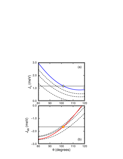
Figure 6: (Color online) Superexchange constants for LaMnO₃: (a) $J_{c}$ along the $c$ axis, and (b) $J_{ab}$ in the $ab$ plane, as functions of orbital angle $\theta$ which defines the $C$-type OO, see Eqs. (III.2). Dashed lines for increasing $R=0$, 0.15 and 0.30 from bottom to top; solid lines for $R=0.6$. Note that the dependence of $J_{ab}$ on $R$ is nonmonotonic. Horizontal dotted lines indicate the experimental values of Ref. Mou96, for LaMnO₃; diamond and circle show the experimental values of $J_{c}$ and $J_{ab}$ for $\theta=102^{\circ}$. Parameters: $J=150$ meV, $\eta=0.181$.

After these two parameter values have been fixed, it is of interest to investigate the dependence of the effective exchange interactions on the CT parameter $R$ and on the orbital angle $\theta$. As in the KCuF₃ case, one finds a stronger increase of $J_{c}$ with increasing $R$, while these terms are weaker and lead to nonmonotonic changes for $J_{ab}$ (Fig. 6). First of all, with the present value of $\eta=0.181$, at $R=0$ the AF interaction $J_{c}$ is close to zero for angles $\theta\sim 100^{\circ}$, while the FM interaction $J_{ab}<-2$ meV is somewhat too strong. With increasing $R$ one finds that $J_{c}$ increases, while the FM interaction $J_{ab}$ initially becomes weaker when $R$ increases up to $R=0.3$ and the term $\propto c_{1}$ dominates the CT contribution to $J_{ab}$ [see Eq. (68)]. At higher values of $R$, however, the FM contributions due to $c_{3}-c_{2}<0$ and $c_{5}-c_{4}<0$ start to dominate, and $J_{ab}$ decreases with increasing $R$, particularly for small values of $\theta<90^{\circ}$. One finds that the experimental values of both exchange constants are well reproduced for $R=0.6$ and at the orbital angle $\theta=102^{\circ}$.

Although this fit is not unique, one has to realize that the experimental constraints imposed on the parameters are indeed rather severe — as we show below the present parameters give a very reasonable and consistent interpretation of the experimental results for LaMnO₃. For the above parameters the FM and AF terms to $J_{c}$ almost compensate each other in the $U$ term, and a considerable AF interaction along the $c$ axis arises mainly due to the CT contributions (Fig. 7). This qualitatively agrees with the situation found in KCuF₃, where the CT term was of crucial importance and helped to explain the observed large anisotropy between the values of exchange constants. Also the CT term which contributes to $J_{ab}$ is AF and increases with increasing angle $\theta$, while the $U$ term is FM but weakens at the same time. This results in a quite fast dependence of the FM interaction $J_{ab}$ on $\theta$ (Fig. 7).

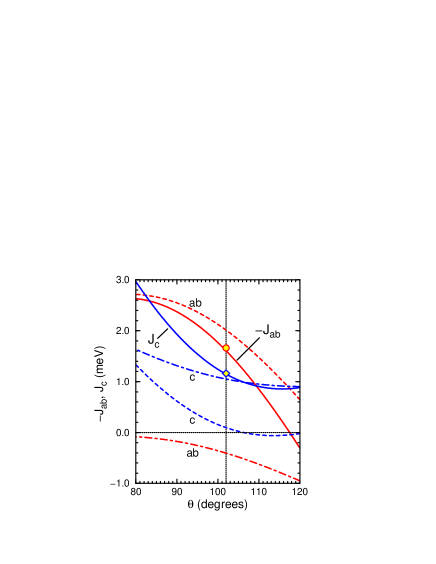
Figure 7: (Color online) Superexchange interactions $-J_{ab}$ (68) and $J_{c}$ (69) as functions of the orbital angle $\theta$, obtained within the superexchange model (47) for LaMnO₃ (solid lines). Contributions due to the $U$ term and due to the CT term to both exchange constants ($-J_{ab}$ and $J_{c}$) are shown by dashed and dashed-dotted lines, respectively. Isotropic and orbital independent $t_{2g}$ terms superexchange terms $J_{tU}$ and $J_{t\Delta}$ (66) are: 1.45 and 0.83 meV. Experimental values Mou96 of $-J_{ab}$ and $J_{c}$ (indicated by diamond and circle) are well reproduced at angle $\theta=102^{\circ}$. Parameters $J=150$ meV, $\eta=0.181$, $R=0.6$.

One thus recognizes a similar dependence of the exchange constants $-J_{ab}$ and $J_{c}$ on the orbital angle $\theta$ (Fig. 7) as that found before with the $U$ term alone (see Fig. 15 in Appendix A). The CT terms have mainly two consequences: (i) a large AF contribution to the interaction along the $c$ axis $J_{c}$, and (ii) an increase of the orbital angle well above $\theta=90^{\circ}$. These trends are robust in the realistic parameter range. Therefore, one expects that the occupied $e_{g}$ orbitals approach the frequently assumed alternating directional orbitals in the $ab$ planes $(3x^{2}-r^{2})/(3y^{2}-r^{2})$ with $\theta=120^{\circ}$, but cannot quite reach them. Indeed, we have verified that orbitals with $\theta\sim 120^{\circ}$ are excluded by the present calculations, as then the FM interaction within the $ab$ planes changes sign and becomes weakly AF. Thus, the mechanism for the observed $A$-AF phase is lost, and one has to conclude that angles $\theta>\theta_{\rm JT}$ are excluded.

Indeed, we have found that the orbital angle $\theta\simeq 102^{\circ}$ reproduces well the experimental data for both exchange constants (Fig. 7), and is thus somewhat smaller than the angle $\theta_{\rm JT}=108^{\circ}$ deduced from the lattice distortions in LaMnO₃.Rod98 This can be seen as a compromise between the orbital interactions involving the lattice and the purely electronic superexchange orbital interactions, so it is reasonable to expect that $\theta<\theta_{\rm JT}$.

Finally, we emphasize that the $e_{g}$ electron excitations, contributing both to the $U$ and to the CT processes in the superexchange, are FM for all cubic directions,noteeg and only due to a substantial $t_{2g}$ term which follows from low-spin (AF) excitations, $J_{t}=2.28$ meV, the exchange interaction along the $c$ axis changes its sign and becomes AF. Alltogether, the present analysis shows that the $t_{2g}$ superexchange plays a decisive role in stabilizing the observed $A$-AF spin order — without it already the undoped LaMnO₃ would be a ferromagnet. This peculiar situation follows from the large splitting between the high-spin and low-spin excitations $\sim 3$ eV in LaMnO₃, which is larger than in any other transition metal compound considered in this paper, due to the fact that the $d$ shell is half-filled in the Mn²⁺ excited states.Ole01 This leads to relatively large FM contributions, even when the orbitals are not so close to the ideal alternation of directional and planar states (as found along the $c$ axis), which would maximize the averages of the orbital operators, $\big{\langle}\frac{1}{4}-\tau_{i}^{(\gamma)}\tau_{j}^{(\gamma)}\big{\rangle}$, that control the weight of the high-spin terms, see Table 2. This result is remarkable but again qualitatively the same as found in the effective model of Appendix A. However, quantitatively the $t_{2g}$ term is here somewhat stronger, as $J_{t}$ is now increased by $\sim 35$% over its value $J_{t}=1.7$ meV deduced from the effective $d-d$ model with $U$ terms only. As a common feature one finds that $J_{t}\sim 2$ meV, so we emphasize that the superexchange promoted by $t_{2g}$ electrons is quite weak and is characterized by a small value of $J_{t}\sim 4\times 10^{-3}t$ (or $\sim 0.01t$ for the superexchange between $S=3/2$ core spins Dag02 ; vdB99 ) which provides an important constraint for the realistic models of manganites.

IV.4 Optical spectral weights in LaMnO₃

Consider now the temperature dependence of the optical spectral weights (15). As the orbital dynamics is quenched up to room temperature $T\sim 300$ K, it suffices to consider the temperature dependence of the intersite spin-spin correlations (12). We derived these by employing the so-called Oguchi methodOgu60 (see Appendix B), which is expected to give rather realistic values of spin correlations functions for the large spins $S=2$ in LaMnO₃ in the entire temperature range. Thereby we solved exactly the spin-spin correlations $\{s_{ab},s_{c}\}$ on a single bond $\langle ij\rangle$ coupled to neighboring spins by mean-field (MF) terms, proportional to the order parameter $\langle S^{z}\rangle$. A realistic estimate of the magnetic transition can be obtained by reducing the MF result obtained for $S=2$ spins by an empirical factor $\sim 0.71$.Fle04 Using the exchange interactions obtained with the present parameters, one finds $T_{N}\simeq 143$ K which reasonably agrees with the experimental value of $T_{N}^{\rm exp}=136$ K.Mou96 The calculations of spin-spin correlations are straightforward, and we summarize them in Appendix B. Both correlation functions $s_{ab}$ and $s_{c}$ change fast close to $T_{N}$, reflecting the temperature dependence of the Brillouin function which deterimes $\langle S^{z}\rangle$, and remain finite at $T\gg T_{N}$.

The large splitting between the high-spin and low-spin excitations makes it possible to separate the high-spin excitations from the remaining ones in the optical spectra, and to observe the temperature dependence of its intensity for both polarizations. As in the effective model,Kov04 ; Ole04 the present theory predicts that the low-energy optical intensity exhibits a rather strong anisotropy between the $ab$ and $c$ directions. It is particularly pronounced and close to 10:1 at low temperatures when the spin correlations $|s_{ab}|$ and $s_{c}$ are maximal (Fig. 8). Unfortunately, this anisotropy at $T\to 0$ in only weakly dependent on the orbital angle $\theta$, so it cannot help to establish the type of OO realized in the ground state of LaMnO₃, and its possible changes with increasing temperature. In fact, when the parameters are fixed and only the orbital angle $\theta$ is changed, a different value of the Néel temperature follows from the modified exchange constants, being the main reason behind the somewhat different temperature dependence of the ratio $K_{1}^{(ab)}/K_{1}^{(c)}$ (Fig. 8).

Figure 8: (Color online) Anisotropy of the low-energy spectral weights in LaMnO₃, given by the ratio $K_{1}^{(ab)}/K_{1}^{(c)}$, for increasing temperature $T$, as obtained for: $\theta=102^{\circ}$ (solid line), $\theta=108^{\circ}$ (dashed line), $\theta=98^{\circ}$ (dashed-dotted line). The arrows indicate the Néel temperature $T_{N}$ derived from the exchange constants in each case (see text). Parameters: $J=150$ meV, $\eta=0.181$.

One finds a very satisfactory agreement between the present theory and the experimental results of Ref. Kov04, , as shown in Fig. 9. We emphasize, however, that the temperature variation of the optical spectral weights could also be reproduced within the effective model at $R=0$,Kov04 ; Ole04 showing that the CT terms lead only to minor quantitative modifications. Note also that at this stage no fit is made, i.e., the kinetic energies (13) which stand for the optical sum rule are calculated using the same parameters as found above to reproduce the exchange constants in Fig. 7. Therefore, such a good agreement with experiment demonstrates that indeed the superexchange interactions describe the spectral intensities in the optical transitions. We note, however, that the anisotropy in the range of $T>T_{N}$ is somewhat larger in experiment which might be due to either some inaccuracy of the Oguchi method or due to the experimental resolution.

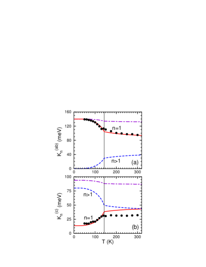
Figure 9: (Color online) Kinetic energies per bond (in meV) as functions of temperature $T$, obtained for LaMnO₃ for the high-spin (solid lines, $n=1$) and for the low-spin (dashed lines, $n>1$) excitations at the Mn ions for polarization: (a) in the $ab$ planes, $K_{n}^{(ab)}$, and (b) along the $c$ axis, $K_{n}^{(c)}$. The total kinetic energies $K^{(\gamma)}$ are given by the long dashed-dotted lines, while the vertical dotted lines indicate the value of $T_{N}$ derived within the present model (see text). Filled circles show the experimental intensities Kov04 at low energy ($n=1$). Parameters: $J=150$ meV, $\eta\simeq 0.181$, $R=0.6$, and $\theta\simeq 102^{\circ}$.

The distribution of the optical intensities $K_{n}^{(\gamma)}$ and their changes between the low ($T\simeq 0$) and the high temperature ($T=300$ K) regime are summarized in Table 4. At temperature $T=0$ one finds that for the $ab$ polarization the entire spectral intensity originates from high-spin excitations. This result follows from the classical value of the spin-spin correlation function $s_{ab}=-1$ predicted by the Oguchi method. As quantum fluctuations in the $A$-AF phase are small,Rac02 the present result is nearly accurate. When the temperature increases, one finds considerable transfer of optical spectral weights between low and high energies, discussed also in Ref. Kov04, , with almost constant total intensities $K^{(\gamma)}$ for both $\gamma=ab$ and $c$ (see also Fig. 9). The optical weights obtained for the JT angle $\theta_{\rm JT}=108^{\circ}$ are similar to those for $\theta=102^{\circ}$, showing again that the optical spectroscopy is almost insensitive to small changes of the orbital angle. In contrast, for $\theta_{\rm JT}$ the exchange constants (and hence also the estimated value of $T_{N}$) are too low.

Table 4: Exchange constants $J_{\gamma}$ [see Eqs. (68) and (69)], kinetic energies for high-spin ($K_{1}^{(\gamma)}$) and for low-spin ($K_{\rm LS}^{(\gamma)}$) excitations [see Eqs. (70)–(73)], and total kinetic energies $K_{\rm tot}^{(\gamma)}$ (all in meV), for a bond within an $ab$ plane ($\gamma=ab$) and along a $c$ axis ($\gamma=c$), as obtained for the OO given by the orbital angle $\theta\simeq 102^{\circ}$ which reproduces the experimental exchange constants,Mou96 and for the angle suggested by the lattice distortions, $\theta_{\rm JT}$. Parameters: $J=150$ meV, $\eta\simeq 0.181$, $R=0.6$.

		$\theta\simeq 102^{\circ}$		$\theta_{\rm JT}=108^{\circ}$
	$T$ (K)	$0$	$300$	$0$	$300$
	$J_{ab}$	$-1.66$		$-1.06$
	$J_{c}$	$1.16$		$0.95$
	$K_{1}^{(ab)}$	140.1	94.2	135.8	88.1
	$K_{\rm LS}^{(ab)}$	0.0	38.1	0.0	42.1
	$K_{\rm tot}^{(ab)}$	140.1	132.3	135.8	130.2
	$K_{1}^{(c)}$	13.7	42.9	12.6	41.2
	$K_{\rm LS}^{(c)}$	80.0	44.0	74.9	40.1
	$K_{\rm tot}^{(c)}$	93.7	86.9	87.5	81.3

While the effective parameters $\{J,\eta,R\}$ used in this Section give a very satisfactory description of both magnetic and optical properties of LaMnO₃, the values of the microscopic parameters, such as the Coulomb interaction on the Mn ions $U$, and on the oxygen ions $U_{p}$, the Hund’s exchange $J_{H}$, the charge transfer parameter $\Delta$, and the $d-p$ hopping element $t_{pd}$, are not uniquely determined. One could attempt to fix these parameters using the atomic value of Hund’s exchange $J_{H}=0.9$ eV. With $\eta=0.181$ it leads to $U\simeq 5.0$ eV, quite close to other estimates,Miz96 while the value of $R=0.6$ suggests then that, taking the commonly acceptedMiz96 ; Boc92 value of the CT energy $\Delta=5.0$ eV, the oxygen Coulomb element is large, $U_{p}\simeq 7$ eV. This value of $U_{p}$ is larger than usually obtained $U_{p}\sim 4$ eV for oxygen ions, as for instance by analyzing the parameters of the three-band model for CuO₂ planes.Gra92 We note, however, that the optical dataKov04 suggest a somewhat reduced value of Hund’s exchange $J_{H}\sim 0.7$ eV (using the present units), so it could be that the local exchange interactions are somewhat screened in reality.

Fortunately, when the optical data are available, also the position of the low-energy excitation is known, and this may serve as an additional experimental constraint for the parameters.Kha04 This excitation is found at about 2.0 eV,Kov04 indicating that $U-3J_{H}\simeq 2.0$ eV. With this constraint one finds, using again $\eta=0.181$, that $U\simeq 3.7$ eV and $J_{H}\simeq 0.67$ eV. These parameters give the low-spin ${}^{4}\!A_{1}$ and ${}^{4}E$ excitations close to 4.5 eV, in agreement with experiment.Kov04 So the above values of the microscopic parameters $\{U,J_{H}\}$ appear to be consistent both with the present value of $\eta$ and with the spectra. Furthermore, for these empirical parameters one finds $R=0.6$ either with $\Delta=5.0$ and $U_{p}\simeq 2.3$ eV, or with $\Delta=4.2$ and $U_{p}\simeq 4.0$ eV. These values, particularly the second set, are perfectly acceptable and in the usually considereed range.Zaa90 ; Boc92 Taking the above value of $U\simeq 3.7$ and $J=150$ meV, one finds $t=0.37$ eV, a somewhat lower value than that which follows from the effective model of Appendix A. Altogether, these results indicate, contrary to what is frequently assumed, Zaa90 ; vdM88 that the local exchange interactions are somewhat screened in reality by covalency effects, and that at the same time the screening of the intraorbital Coulomb interaction $U$ is stronger than estimated before.Miz96 ; Boc92

V Cubic titanites

V.1 Spin-orbital superexchange model

Perovskite titanates, LaTiO₃ and YTiO₃, are intriguing examples of Mott insulators with orbital degrees of freedom due to $t_{2g}$ electrons: in the ground state the Ti³⁺ ions are in the $t_{2g}^{1}$ configuration. In an ideal perovskite structure the $t_{2g}$ orbitals are degenerate, but lattice distortions may contribute to the magnetic ground stateCwi03 ; Moc03 ; Sol04 ; Pav05 and to the Mott transition Pav04 — here we do not intend to discuss this controversial issue.

In an ideal cubic system each $t_{2g}$ orbital is perpendicular to a single cubic axis, for instance the $|xy\rangle$ orbital lies in the $ab$ plane and is perpendicular to the $c$ axis. It is therefore convenient to introduce the following short hand notation for the orbital degree of freedom:Kha00

$$|a\rangle\equiv|yz\rangle,\hskip 19.91684pt|b\rangle\equiv|zx\rangle,\hskip 19.91684pt|c\rangle\equiv|xy\rangle.$$ (74)

The labels $\gamma=a,b,c$ thus refer to the cubic axes perpendicular to the planes of the respective orbitals.

The superexchange spin-orbital model (8) in cubic titanates couples $S=1/2$ spins and the orbital $t_{2g}$ degrees of freedom at nearest neighbor Ti³⁺ ions. Due to large $U$ the electron densities satisfy thereby the local constraint at each site $i$,

$$n_{ia}+n_{ib}+n_{ic}=1.$$ (75)

In titanates there is no need to consider CT processes, as these systems are Mott-Hubbard insulatorsIma98 and no qualitatively new effects apart from some negligible renormalization of the effective parameters $\{J,\eta\}$ could arise from CT excitations. This simplifies our considerations, so we analyze the superexchange in the leading order of perturbation theory, given by the contributions which result from virtual excitations between the neighboring Ti³⁺ ions, $(t_{2g}^{1})_{i}(t_{2g}^{1})_{j}\rightleftharpoons(t_{2g}^{2})_{i}(t_{2g}^{0})_{j}$. These charge excitations involve the Coulomb interactions in the $d^{2}$ configuration of a Ti²⁺ ion, parametrized as before by the intraorbital Coulomb element $U$, and by Hund’s exchange element $J_{H}$ for a pair of $t_{2g}$ electrons, defined as follows (see Table 1),Gri71

$$J_{H}=3B+C.$$ (76)

The charge excitations lead to one of four different excited states Gri71 shown in Fig. 1(b): the high-spin ${}^{3}T_{1}$ state at energy $U-3J_{H}$, and three low-spin states — degenerate ${}^{1}T_{2}$ and ${}^{1}E$ states at energy $U-J_{H}$, and an ${}^{1}\!A_{1}$ state at energy $U+2J_{H}$. As before, the excitation energies are parameterized by $\eta$, defined as in Eq. (19), and we introduce the coefficients

$$r_{1}=\frac{1}{1-3\eta},\hskip 14.22636ptr_{2}=\frac{1}{1-\eta},\hskip 14.22636ptr_{3}=\frac{1}{1+2\eta}.$$ (77)

One finds the following compact expressions for the superexchange ${\cal H}_{U}(d^{1})$ as given by Eq. (6):Kha00 ; Kha03

$$H_{1}^{(\gamma)}\! = \!\frac{1}{2}Jr_{1}\Big{(}\vec{S}_{i}\!\cdot\!\vec{S}_{j}+\frac{3}{4}\Big{)}\Big{(}A_{ij}^{(\gamma)}\!-\frac{1}{2}n_{ij}^{(\gamma)}\Big{)},$$ (78)

$$H_{2}^{(\gamma)}\! = \!\frac{1}{2}Jr_{2}\Big{(}\vec{S}_{i}\!\cdot\!\vec{S}_{j}-\frac{1}{4}\Big{)}\Big{(}A_{ij}^{(\gamma)}\!-\frac{2}{3}B_{ij}^{(\gamma)}\!+\frac{1}{2}n_{ij}^{(\gamma)}\Big{)},$$

$$H_{3}^{(\gamma)}\! = \!\frac{1}{3}Jr_{3}\Big{(}\vec{S}_{i}\!\cdot\!\vec{S}_{j}-\frac{1}{4}\Big{)}B_{ij}^{(\gamma)},$$ (80)

where

$$A_{ij}^{(\gamma)} = 2\Big{(}\vec{\tau}_{i}\cdot\vec{\tau}_{j}+\frac{1}{4}n_{i}n_{j}\Big{)}^{(\gamma)},$$ (81)

$$B_{ij}^{(\gamma)} = 2\Big{(}\vec{\tau}_{i}\otimes\vec{\tau}_{j}+\frac{1}{4}n_{i}n_{j}\Big{)}^{(\gamma)},$$ (82)

$$n_{ij}^{(\gamma)} = n_{i}^{(\gamma)}+n_{j}^{(\gamma)}.$$ (83)

As in Secs. III and IV the orbital (pseudospin) operators $\{A_{ij}^{(\gamma)},B_{ij}^{(\gamma)},n_{ij}^{(\gamma)}\}$ depend on the direction of the $\langle ij\rangle$ bond. Their form follows from the simple observationKha00 ; Har03 that only two $t_{2g}$ orbitals (flavors) are active along each cubic axis, e.g. if $\gamma=c$, the active orbitals are $a$ and $b$ [see Eq. (74)], and they give two components of the pseudospin $T=1/2$ operator $\vec{\tau}_{i}$. Here the operators $\{A_{ij}^{(\gamma)},B_{ij}^{(\gamma)}\}$ describe the interactions between the active orbitals along the particular bond, which include the quantum effects due to their fluctuations, and take either the form of a scalar product $\vec{\tau}_{i}\cdot\vec{\tau}_{j}$, or lead to a similar expression,

$$\vec{\tau}_{i}\otimes\vec{\tau}_{j}=\tau_{i}^{x}\tau_{j}^{x}-\tau_{i}^{y}\tau_{j}^{y}+\tau_{i}^{z}\tau_{i}^{z},$$ (84)

which involves double excitations due to $\tau_{i}^{+}\tau_{j}^{+}$ and $\tau_{i}^{-}\tau_{j}^{-}$ terms (as in the $U<0$ Hubbard model). The interactions along axis $\gamma$ are tuned by the number of electrons occupying active orbitals, $n_{i}^{(\gamma)}=1-n_{i\gamma}$, which is fixed by the number of electrons in the inactive orbital $n_{i\gamma}$, because of the constraint (75).

V.2 Spin exchange constants and optical intensities

The exchange constant for a bond $\langle ij\rangle$ along axis $\gamma$ is obtained from Eqs. (78)–(80) by averaging over the orbital states at both sites $i$ and $j$,

$$J_{\gamma} = \frac{1}{2}J(r_{1}+r_{2})\Big{\langle}A_{ij}^{(\gamma)}\Big{\rangle}-\frac{1}{3}J(r_{2}-r_{3})\Big{\langle}B_{ij}^{(\gamma)}\Big{\rangle}$$ (85)

$$- \frac{1}{4}J(r_{1}-r_{2})\Big{\langle}n_{i}^{(\gamma)}+n_{j}^{(\gamma)}\Big{\rangle}.$$

The cubic titanates are known to have particularly pronounced quantum spin-orbital fluctuations, and their proper treatment requires a rather sophisticated approach.Kha00 ; Kha03 Here we shall ignore this complex quantum problem, and shall illustrate the general theory by extracting the magnetic exchange constants from Eq. (85), and the optical spectral weights (15), using an ansatz for the OO in the ground state, in analogy to the approach employed in Secs. III and IV for the more classical $e_{g}$ systems.

In general a classical orbital state in the titanates with GdFeO₃-type lattice structure can be parametrized as follows,

$$|\psi_{1}\rangle = \alpha|a\rangle+\beta|b\rangle+\gamma|c\rangle,$$

$$|\psi_{2}\rangle = \beta|a\rangle+\alpha|b\rangle+\gamma|c\rangle,$$

$$|\psi_{3}\rangle = \alpha|a\rangle+\beta|b\rangle-\gamma|c\rangle,$$

$$|\psi_{4}\rangle = \beta|a\rangle+\alpha|b\rangle-\gamma|c\rangle,$$ (86)

with real coefficients and normalized ($\alpha^{2}+\beta^{2}+\gamma^{2}=1$) wavefunctions at each site. The occupied orbitals $|\psi_{i}\rangle$ refer to four sublattices ($i=1,\cdots,4$), with Ti${}_{1}(000)$, Ti${}_{2}(100)$, Ti${}_{3}(001)$, Ti${}_{4}(101)$ positions.Miz96 ; Saw97 The minus signs in $|\psi_{3}\rangle$ and $|\psi_{4}\rangle$ reflect a mirror symmetry present in the GdFeO₃ structure. Note that this state resembles $G$-type OO, and is thus different from the $C$-type OO encountered for $e_{g}$ orbitals [due to the change of sign for the $|c\rangle$ orbitals in Eqs. (V.2) along the $c$ axis].

Using the ansatz (V.2) one finds after a straightforward calculation the exchange constants,

$$J_{c} = \frac{1}{2}J\Big{[}(r_{1}+r_{2}r_{3})(1-\gamma^{2})^{2}$$ (87)

$$\hskip 14.22636pt-(r_{1}-r_{2})(1-\gamma^{2})\Big{]},$$

$$J_{ab} = \frac{1}{4}J\Big{[}2(r_{1}+r_{2}r_{3})(\gamma^{2}+\alpha\beta)^{2}$$ (88)

$$\hskip 14.22636pt-(r_{1}-r_{2})(1+\gamma^{2})\Big{]}.$$

They are determined once again by: (i) the superexchange parameter $J$ given by Eq. (7), with $t$ standing now for the effective $(dd\pi)$ hopping element, (ii) Hund’s exchange element $\eta$ (19),noterr and (iii) the orbital state (V.2), specified in the present case by the coefficients $\{\alpha,\beta,\gamma\}$.

Following the general theory of Sec. II, the optical excitations corresponding to the high-spin Hubbard band at energy $U-3J_{H}$ $(n=1)$, and to the two low-spin Hubbard bands at $U-J_{H}$ $(n=2)$ and $U+2J_{H}$ $(n=3)$ of Fig. 1(b), have total intensities given by the respective kinetic energies $K_{n}^{(\gamma)}$, see Eq. (15). Using the classical wavefunctions given by Eqs. (V.2), one finds the following optical spectral weights:
— for polarization along the $c$ axis,

$$K_{1}^{(c)} = Jr_{1}\gamma^{2}(1-\gamma^{2})\Big{(}\frac{3}{4}+s_{c}\Big{)},$$ (89)

$$K_{2}^{(c)} = \frac{4}{3}Jr_{2}(1-\gamma^{2})\Big{(}1-\frac{1}{4}\gamma^{2}\Big{)}\Big{(}\frac{1}{4}-s_{c}\Big{)},$$ (90)

$$K_{3}^{(c)} = \frac{2}{3}Jr_{3}(1-\gamma^{2})^{2}\Big{(}\frac{1}{4}-s_{c}\Big{)},$$ (91)

— for polarization in the $ab$ plane,

$$\hskip-14.22636ptK_{1}^{(ab)}\!\! = \!\!Jr_{1}\Big{[}\frac{1}{2}(1\!+\!\gamma^{2})-(\gamma^{2}\!+\!\alpha\beta)^{2}\Big{]}\Big{(}\frac{3}{4}+\!s_{ab}\Big{)},$$ (92)

$$\hskip-14.22636ptK_{2}^{(ab)}\!\! = \!\!Jr_{2}\Big{[}\frac{1}{2}(1\!+\!\gamma^{2})+\frac{1}{3}(\gamma^{2}\!+\!\alpha\beta)^{2}\Big{]}\Big{(}\frac{1}{4}-\!s_{ab}\Big{)},$$ (93)

$$\hskip-14.22636ptK_{3}^{(ab)}\!\! = \!\!\frac{2}{3}Jr_{3}(\gamma^{2}+\alpha\beta)^{2}\Big{(}\frac{1}{4}-s_{ab}\Big{)}.$$ (94)

The kinetic energies $K_{n}^{(\gamma)}$ depend on the same parameters $\{J,\eta\}$ as the exchange constants (87) and (88), on the orbital state (V.2) via the coefficients $\{\alpha,\beta,\gamma\}$, and on the spin-spin correlations (12).

V.3 Application to LaTiO₃ and YTiO₃

It is now straightforward to investigate the dependence of the magnetic and the optical properties in the four-sublattice classical state (V.2) on the effective parameters $\{J,\eta\}$ and on the type of OO given by the coefficients $\{\alpha,\beta,\gamma\}$. A priori, the average electron density in the $|c\rangle$ orbitals, $n_{c}=\langle n_{ic}\rangle$, is different from the densities in the other two orbitals ($n_{a}$ and $n_{b}$), and the cubic symmetry of the expectation values $J_{\gamma}$ and $K_{n}^{\gamma}$ is explicitly broken by the OO given by Eq. (V.2), unless all the orbital amplitudes are equal,

$$\alpha=\beta=\gamma=\frac{1}{\sqrt{3}},$$ (95)

as argued in Refs. Moc03, ; Cwi03, . First we consider this isotropic state and evaluate the exchange constants $J_{\gamma}$ for increasing Hund’s parameter $\eta$. One finds then AF superexchange $J_{\gamma}\sim 0.4J$ which decreases with increasing $\eta$ [Fig. 10(a)], but the interactions remain AF in the physically relevant range of $\eta<0.28$. Note that this classical consideration seriously overestimates the actual exchange interaction as one expects instead $J_{\gamma}\sim 0.16J$ when quantum effects are included. Kha00 Nevertheless, having no information about the optical excitations, we give here an example of estimating the exchange constants and optical spectral weights using the spectroscopic values Miz96 for Hund’s exchange $J_{H}\simeq 0.59$, and for Coulomb intraorbital interaction of $U=4.8$ eV, which give $\eta=0.123$. Assuming now a hopping parameter $t=0.2$ eV, one finds $J\simeq 33$ meV which gives $J_{\gamma}\simeq 14$ meV. While one might expect that the effective $U$ is somewhat reduced as in the case of LaMnO₃, and the value of $\eta$ would then be larger, the present crude estimate is accidentally quite close to the experimental value of $J_{\rm exp}=15.5$ meV.Kei00

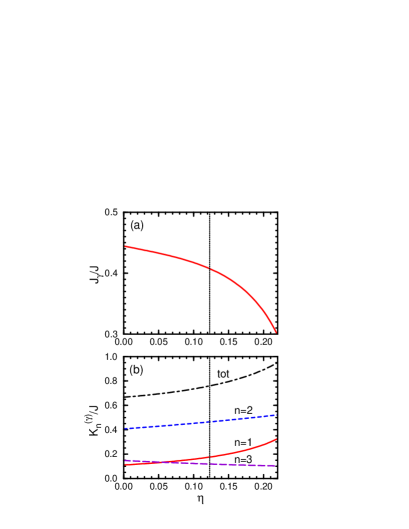
Figure 10: (Color online) Magnetic and optical properties of LaTiO₃, as obtained for the classical wavefunctions (V.2) with isotropic orbital amplitudes (95), for increasing Hund’s exchange $\eta=J_{H}/U$: (a) exchange interactions $J_{c}=J_{ab}$, and (b) kinetic energy terms $K_{n}^{(\gamma)}$ at $T=0$: high-spin ($n=1$, solid line), and low-spin intermediate-energy ($n=2$, dashed line) and high-energy excitation ($n=3$, long-dashed line). The total kinetic energy $K^{(\gamma)}$ is shown by the dashed-dotted line.

In the AF state, realized in LaTiO₃, all three Hubbard subbands contribute in the optical spectroscopy, and taking the Néel state with $s_{ab}=s_{c}=-0.25$ one finds the highest spectral weight at $T=0$ for $n=2$ [Fig. 10(b)]. For the realistic value $\eta\sim 0.123$ the spectral weight of the lowest-energy (high-spin) Hubbard subband $K^{(\gamma)}_{1}$ is relatively weak, and is similar to that of the $n=3$ low-spin excitation at the highest energy [Fig. 10(b)]. Note, however, that in early optical experiments the intensity was found to be practically independent of energy $\omega$,Ari93 so different excitations might be difficult to separate from each other.

Let us verify now whether the wavefunctions as given by Eqs. (V.2) could also lead to isotropic AF states for other choices of orbital amplitudes than in Eq. (95). Thus, we considered equal amplitudes $\alpha$ and $\gamma$ in the states parametrized by $\delta$,

$$\alpha=\gamma=(1-\delta)\frac{1}{\sqrt{3}}+\delta\frac{1}{\sqrt{2}},$$ (96)

with $0<\delta<1$. The normalization condition gives $\beta=(1-\alpha^{2}-\gamma^{2})^{1/2}$ which vanishes at $\delta=1$. As expected, the exchange interactions are anisotropic for small $\delta>0$ (Fig. 11). The increasing occupancy of the $c$ orbitals with increasing $\delta$ results in a somewhat enhanced exchange interaction $J_{ab}$ near the isotropic state (for $\delta<0.5$), while the interaction $J_{c}$ decreases almost linearly.noteli At larger orbital anisotropy the interaction $J_{ab}$ decreases as well. It is remarkable that the AF interactions become again isotropic close to $\alpha=\gamma=1/\sqrt{2}$ which gives a large charge density $n_{c}\simeq 0.5$ in the $|c\rangle$ orbitals, but this feature is not generic and will likely be modified by quantum effects. Note also that the state at $\beta=0$ in not a FM state, contrary to some earlier suggestions.Miz96

Figure 11: Exchange interactions $J_{c}$ and $J_{ab}$, Eqs. (85) (solid and dashed line) for the titanite model for different types of orbital order given by Eqs. (V.2). The coefficients in the wavefunctions (V.2) vary between the isotropic state $\alpha=\beta=\gamma=1/\sqrt{3}$ and the state with linear combinations of $|a\rangle/|b\rangle$ and $|c\rangle$ orbitals, with the coefficients given by: $\alpha=\gamma=1/\sqrt{3}+\delta(1/\sqrt{2}-1/\sqrt{3})$ and $\beta=(1-\alpha^{2}-\gamma^{2})^{1/2}$. Parameters: $\eta=0.123$.

Finally we remark that the temperature dependence of the optical spectral weights can again be studied in a similar way as for LaMnO₃, by solving the spin-spin correlation functions at increasing temperature using the method of Appendix B for $S=1/2$ spins. Having no experimental data neither for LaTiO₃ nor for YTiO₃, we shall limit ourselves to making predictions concerning the overall change of the spectral weights between low temperature $T\sim 0$ where the spin-spin correlations are maximal, and room temperature $T\gg T_{N}$ (or $T\gg T_{C}$), where the spin-spin correlations may be neglected. We take rigid classical wave functions with OO (V.2) and discuss first AF states. Apart from the isotropic AF phase (95), called state $A$, we consider in Table 5 also somewhat modified orbital amplitudes, as proposed by Itoh et al.:Ito99

$$\alpha=0.690,\hskip 19.91684pt\beta=0.452,\hskip 19.91684pt\gamma=0.565,$$ (97)

called here state $B$. One finds that the exchange interactions $J_{c}$ and $J_{ab}$ are then rather anisotropic (see Table 5), so we believe that this state can be experimentally excluded on the basis of the neutron data.Kei00

Table 5: Exchange constants $J_{\gamma}$, kinetic energies for Hubbard subbands $K_{n}^{(\gamma)}$ and total kinetic energies $K^{(\gamma)}$ (all in units of $J$) for two orbital ordered states suggested for LaTiO₃: state $A$ (95), and state $B$ (97) reported in Ref. Ito99, , and for the OO state suggested for YTiO₃ in Ref. Kha03, . Parameter: $\eta=0.123$.

		LaTiO3				YTiO3
		state $A$ (95)		state $B$ (97)		state $F$ (V.3)
		$T=0$	$T\gg T_{N}$	$T=0$	$T\gg T_{N}$	$T=0$	$T\gg T_{C}$
	$J_{c}$	0.407		0.428		-0.148
	$J_{ab}$	0.407		0.351		-0.148
	$K_{1}^{(c)}$	0.176	0.264	0.172	0.258	1.057	0.792
	$K_{2}^{(c)}$	0.465	0.232	0.476	0.238	0.000	0.190
	$K_{3}^{(c)}$	0.118	0.059	0.124	0.062	0.000	0.000
	$K^{(c)}$	0.759	0.555	0.772	0.558	1.057	0.982
	$K_{1}^{(ab)}$	0.176	0.264	0.207	0.311	1.057	0.792
	$K_{2}^{(ab)}$	0.465	0.232	0.451	0.226	0.000	0.190
	$K_{3}^{(ab)}$	0.118	0.059	0.107	0.053	0.000	0.000
	$K^{(ab)}$	0.759	0.555	0.765	0.590	1.057	0.982

Due to the AF order in the ground state for the wavefunctions $A$ and $B$, the lowest energy high-spin excitations are suppressed at low temperature, but we predict that their weight should increase by about $50$% above the magnetic transition (Table 5). An even stronger temperature dependence is predicted for the low-spin part of the spectra with its intensity decreasing by a factor 2 when the magnetic order is lost. Thus, the spectral weight is shifted from the high-energy to the low-energy part of the optical spectrum with increasing temperature, and the total spectral weight decreases, both features being typical of AF bonds. An experimental confirmation of this trend would also allow one to identify the energy splitting between the high-spin and low-spin parts of the upper Hubbard band, and to determine the value of Hund’s exchange $J_{H}$ from experiment. Although the anisotropy in spectral weights found in the state (97) proposed by Itoh et al.Ito99 might be too weak to be seen experimentally, the predicted anisotropy in the exchange interactions is certainly detectable.

It is quite remarkable that an isotropic FM ground state of YTiO₃ can also be described classically by the OO state with four sublattices, but the phase factors in the wavefunctions have to be then selected differently:Kha03

$$|\phi_{1}\rangle = \frac{1}{\sqrt{3}}(|a\rangle+|b\rangle+|c\rangle),$$

$$|\phi_{2}\rangle = \frac{1}{\sqrt{3}}(-|a\rangle-|b\rangle+|c\rangle),$$

$$|\phi_{3}\rangle = \frac{1}{\sqrt{3}}(-|a\rangle+|b\rangle-|c\rangle),$$

$$|\phi_{4}\rangle = \frac{1}{\sqrt{3}}(|a\rangle-|b\rangle-|c\rangle).$$ (98)

We call this state the orbital $F$ state. Neglecting again orbital (quantum) fluctuations, one finds $\langle A_{ij}^{(\gamma)}\rangle=\langle B_{ij}^{(\gamma)}\rangle=0$ in this state, while $n_{i}^{(\gamma)}=\frac{4}{3}$. At finite $\eta$ this leads indeed to an isotropic FM state with exchange constants,

$$J_{c}^{\rm FM}=J_{ab}^{\rm FM}=-\frac{2}{3}J\eta r_{1}r_{2},$$ (99)

in lowest order $\propto\eta$,notefet so this type of OO leads to a markedly different exchange constant from that given by Eq. (87). Assuming again the same parameters as above one finds $J^{\rm FM}_{\gamma}\simeq-5$ meV, which is somewhat higher than the experimental value $J^{\rm exp}_{\gamma}\simeq-3$ meV.Ulr02 However, in view of the simplicity of the present considerations this agreement can be regarded as satisfactory.

Consider now the spectral weights in the optical spectroscopy. One finds rather simple expressions for the (isotropic) optical spectral weights for the $F$ state:

$$K_{1}^{(\gamma)} = \frac{2}{3}Jr_{1}\Big{(}\frac{3}{4}+s_{\gamma}\Big{)},$$ (100)

$$K_{2}^{(\gamma)} = \frac{2}{3}Jr_{2}\Big{(}\frac{1}{4}-s_{\gamma}\Big{)},$$ (101)

$$K_{3}^{(\gamma)} = 0.$$ (102)

Thus, the optical spectrum of YTiO₃ would be quite different from that of LaTiO₃ (see Table 5). For the FM state at $T=0$ (with $s_{\gamma}=\frac{1}{4}$) only the high-spin spectral weight $K_{1}^{(\gamma)}=\frac{2}{3}Jr_{1}$ contributes, and for the present parameters $K_{1}^{(\gamma)}\simeq J$. Thus, future optical experiments on YTiO₃ combined with magnetic experiments could help to determine the superexchange constant $J$. Furthermore, for the FM $F$ orbital state (V.3) one finds at high temperature a moderate reduction of the low-energy spectral weight by $\sim 25$%, and a corresponding increase for the higher energy excitation $n=2$ [the third excitation does not contribute as long as the OO remains the same as in Eqs. (V.3)]. The energy difference between these excitations is $2J_{H}$ (Fig. 1), so they might serve to determine this parameter from the optical spectroscopy.

The above results show once again that the magnetic interactions and the optical spectral weights depend in a crucial way on the underlying orbital state. Once the OO in $F$ state (V.3) has been fixed, the exchange constants $J_{c}^{\rm FM}$ (99) were completely determined by the superexchange $J$ (7), and by Hund’s exchange parameter $\eta$. For the optical spectral weights $K_{n}^{(\gamma)}$ (100)–(102) one needs in addition the spin-spin correlation function $s_{\gamma}$. Most importantly, a strong temperature dependence of the optical spectra follows here from a classical orbital picture, and this should be a crucial experimental test of the validity of the present approach.

VI Cubic vanadates

VI.1 Spin-orbital superexchange model

The last example of spin-orbital physics we want to give here are the cubic vanadates, in which the orbital degrees of freedom originate from the $t_{2g}^{2}$ configuration of the V³⁺ ions present in the ground state. Here our goal will be to answer the question to what extent these systems could be described by decoupling spin and orbital degrees of freedom and assuming classical states with OO. The OO in the cubic vanadates is complementary to the spin order — the $C$-type AF phase is found for $G$-type OO, and the $G$-type AF phase is accompanied by $C$-type OO.Miy03 Here we shall consider in more detail $G$-type OO, relevant for the case of LaVO₃. We will show in particular that the superexchange spin-orbital modelKha01 allows one to understand the microscopic reasons behind the $C$-AF phase observed in LaVO₃, and predicts that $|J_{c}|\sim J_{ab}$, as actually observed.Kei05 The comparable size of FM and AF exchange constants $J_{c}$ and $J_{ab}$, respectively, is unexpected when considering the Goodenough-Kanamori-Anderson rules,Goode which would suggest that $|J_{c}|$ is by a factor $J_{H}/U$ smaller.

In the case of the vanadates the superexchange between the $S=1$ spins of V³⁺ ions in a perovskite lattice results from virtual charge excitations $(t_{2g}^{2})_{i}(t_{2g}^{2})_{j}\rightleftharpoons(t_{2g}^{3})_{i}(t_{2g}^{1})_{j}$. These charge excitations involve the Coulomb interactions in the $d^{3}$ configuration of a V²⁺ ion, parametrized for a pair of $t_{2g}$ electrons, as for the titanates, by the intraorbital Coulomb element $U$, and by Hund’s exchange element $J_{H}$ [see Eq. (76) and Table 1].Gri71 The excitation spectrum which leads to the superexchange model includes three states:Kha01 (i) a high-spin state ${}^{4}\!A_{2}$ at energy $U-3J_{H}$, (ii) two degenerate low-spin states ${}^{2}T_{1}$ and ${}^{2}E$ at energy $U$, and (iii) a ${}^{2}T_{2}$ low-spin state at energy $U+2J_{H}$ (Fig. 1). We parametrize it by two coefficients: $r_{1}=1/(1-3\eta)$ and $r_{3}=1/(1+2\eta)$. A general Hamiltonian was already given in Ref. Kha01, ; here we shall analyze it assuming that the $xy$ ($|c\rangle$) orbitals are singly occupied at each V³⁺ ion, as concluded from experimentMah92 ; Bla01 and from electronic structure calculations.Saw96 Therefore, the electron densities in the remaining two orbitals satisfy at each site $i$ the local constraint,

$$n_{ia}+n_{ib}=1.$$ (103)

One finds then that the superexchange ${\cal H}_{U}(d^{2})$ for a bond ${\langle ij\rangle}$ along the $c$ axis consists of

$$H_{1}^{(c)} = -\frac{J}{3}r_{1}(2+\vec{S}_{i}\!\cdot\!\vec{S}_{j})\Big{(}\frac{1}{4}-\vec{\tau}_{i}\cdot\vec{\tau}_{j}\Big{)},$$ (104)

$$H_{2}^{(c)} = -\frac{J}{12}(1-\vec{S}_{i}\!\cdot\!\vec{S}_{j})$$ (105)

$$\times\Big{(}\frac{7}{4}-\tau_{i}^{z}\tau_{j}^{z}-\tau_{i}^{x}\tau_{j}^{x}+5\tau_{i}^{y}\tau_{j}^{y}\Big{)},$$

$$H_{3}^{(c)} = -\frac{J}{4}r_{3}(1-\vec{S}_{i}\!\cdot\!\vec{S}_{j})$$ (106)

$$\times\Big{(}\frac{1}{4}+\tau_{i}^{z}\tau_{j}^{z}+\tau_{i}^{x}\tau_{j}^{x}-\tau_{i}^{y}\tau_{j}^{y}\Big{)},$$

and for a bond in the $ab$ plane,

$$H_{1}^{(ab)} = -\frac{1}{6}Jr_{1}\Big{(}\vec{S}_{i}\!\cdot\!\vec{S}_{j}+2\Big{)}\Big{(}\textstyle{\frac{1}{4}}-\tau_{i}^{z}\tau_{j}^{z}\Big{)}.$$ (107)

$$H_{2}^{(ab)} = -\frac{1}{8}J\Big{(}1-\vec{S}_{i}\!\cdot\!\vec{S}_{j}\Big{)}$$ (108)

$$\times\Big{(}\frac{19}{12}\mp\frac{1}{2}\tau_{i}^{z}\mp\frac{1}{2}\tau_{j}^{z}-\frac{1}{3}\tau_{i}^{z}\tau_{j}^{z}\Big{)},$$

$$H_{3}^{(ab)} = -\frac{1}{8}Jr_{3}\Big{(}1-\vec{S}_{i}\!\cdot\!\vec{S}_{j}\Big{)}$$ (109)

$$\times\Big{(}\frac{5}{4}\mp\frac{1}{2}\tau_{i}^{z}\mp\frac{1}{2}\tau_{j}^{z}+\tau_{i}^{z}\tau_{j}^{z}\Big{)},$$

where the operators $\vec{\tau}_{i}$ describe orbital pseudospins $T=1/2$ defined (for each direction $\gamma$) by the orbital doublet $\{|yz\rangle,|xz\rangle\}\equiv\{|a\rangle,|b\rangle\}$. At each site $i$ there is precisely one electron in these two orbitals, and both of them are active along the $c$ axis.

It has already been shown beforeKha04 that the quantum fluctuations play a decisive role in LaVO₃, and the observed Miy02 anisotropy and temperature dependence of the high-spin excitations in optical spectroscopy is reproduced when the theory includes them. In the next Sec. VI.2 we will present now the limitations of a simplified approach which is widely accepted Bla01 and assumes that the OO in LaVO₃ is quite rigid already at the magnetic transition. Quantum fluctuations lead to important corrections which go beyond this picture and modify the temperature variation of the optical spectral weights, as we discuss in Sec. VI.3.

VI.2 Spin exchange constants and optical spectral weights for alternating orbital order

After decoupling of spin and orbital variables, the effective spin exchange constants $J_{c}$ and $J_{ab}$ in Eq. (11) can be obtained from Eqs. (104)–(109) by averaging over orbital correlations, as derived in Ref. Kha04, ,

$$J_{c} = -\frac{1}{2}J\Big{[}\eta r_{1}-(r_{1}-\eta r_{1}-\eta r_{3})$$ (110)

$$\times\Big{(}\frac{1}{4}+\langle\vec{\tau}_{i}\!\cdot\!\vec{\tau}_{j}\rangle\Big{)}-2\eta r_{3}\langle\tau_{i}^{y}\tau_{j}^{y}\rangle\Big{]},$$

$$J_{ab} = \frac{1}{4}J\Big{[}1-\eta r_{1}-\eta r_{3}$$ (111)

$$+(r_{1}-\eta r_{1}-\eta r_{3})\Big{(}\frac{1}{4}+\langle\tau_{i}^{z}\tau_{j}^{z}\rangle\Big{)}\Big{]}.$$

They are determined by the orbital correlations, which result not only from the superexchange ${\cal H}_{U}(d^{2})$ but also from the interactions with the lattice (from the JT term),Kha04 as discussed in detail in Sec. VI.3. Here we shall consider first classical states with alternating $|a\rangle$ and $|b\rangle$ orbitals in the $ab$ planes: $G$-type OO when these orbitals alternate also along the $c$ axis, and $C$-type OO for repeated either $|a\rangle$ or $|b\rangle$ orbitals along the $c$ axis. These classical states are frequently assumed as a consequence of a strong JT term and observed GdFeO₃ distortions. Bla01 Such classical order would naturally follow from a strong JT effect, but it is still controversial whether the JT interaction is actually that strong in the vanadates. Fortunately, there are already experimental results which can help to resolve this controversy, and we address this issue in more detail in Sec. VI.3.

First we consider the limit of strong JT interaction with rigid OO. This implies $\langle\vec{\tau}_{i}\!\cdot\!\vec{\tau}_{j}\rangle\simeq\langle\tau_{i}^{z}\tau_{j}^{z}\rangle=-\frac{1}{4}$ along each bond for $G$-type OO, so one finds from Eqs. (110) and (111) fixed values of the exchange constants:

$$J_{c}^{C-{\rm AF}} = -\frac{1}{2}J\eta r_{1},$$ (112)

$$J_{ab}^{C-{\rm AF}} = \frac{1}{4}J[1-\eta(r_{1}+r_{3})].$$ (113)

The FM interaction $J_{c}^{C-{\rm AF}}$ increases in lowest order linearly with Hund’s exchange $\eta$, and the above values of the exchange constants give $C$-AF spin order.

Whether or not such a classical OO is realized in the ground state, can be investigated by analyzing the consequences of the present theory for the distribution of spectral weight in the optical spectroscopy. The optical spectral weights follow by averaging the individual contributions to the superexchange, see Eqs. (13) and (15). One finds for $G$-type OO the optical spectral weights:
— for polarization along the $c$ axis,

$$K_{1}^{(c)} = \frac{1}{3}Jr_{1}\big{(}s_{c}+2\big{)},$$ (114)

$$K_{2}^{(c)} = \frac{1}{3}J\big{(}1-s_{c}\big{)},$$ (115)

$$K_{3}^{(c)} = 0,$$ (116)

— for polarization in the $ab$ plane,

$$K_{1}^{(ab)} = \frac{1}{6}Jr_{1}\big{(}s_{ab}+2\big{)},$$ (117)

$$K_{2}^{(ab)} = \frac{5}{12}J\big{(}1-s_{ab}\big{)},$$ (118)

$$K_{3}^{(ab)} = \frac{1}{4}Jr_{3}\big{(}1-s_{ab}\big{)}.$$ (119)

As in all other cases, they depend on two model parameters, $J$ and $\eta$, and on the spin-spin correlations $\{s_{c},s_{ab}\}$ (the OO is already fixed).

Again, as in the case of LaMnO₃ (Sec. IV), the analysis of the optical spectra suggests that the effective parameters are somewhat different from the atomic values, primarily due to the screening of both Coulomb $U$ and Hund’s exchange $J_{H}$. We use here the parameters deduced from the neutron experimentsUlr03 and from the optical spectraMiy02 — one findsKha04 $J=40$ meV and $\eta=0.13$. These values imply that $J_{c}\simeq-4.3$ meV and $J_{ab}\simeq 6.8$ meV, which lead to a MF estimate of the transition temperature $T_{N}^{\rm MF}\simeq 270$K. This value has to be still reduced by an empirical factorFle04 (close to 68% for $S=1$) to estimate the effect of thermal fluctuations, so one finds $T_{N}\sim 180$ K in reasonable agreement with the experimental value of 140 K. Miy00 We note that the above values of the exchange constants are in good agreement with the neutron experiments.Kei05

It is instructive to test this classical approach by analyzing its predictions for the optical spectral weights. We evaluated the spin correlation functions for bonds in the $ab$ plane and along the $c$ axis using the Oguchi method, and used an order parameter $\langle S^{z}\rangle$ at neighboring sites, which acts on the considered bond by MF terms and vanishes at $T_{N}=0.4J$, as explained in Ref. Kha04, . The correlation $s_{c}$ for FM bonds along the $c$ axis can be obtained analytically,Kha04 while $s_{ab}$ for the AF bonds was determined by a numerical approach described in Appendix C. As expected, the spectral weight due to the high-spin excitations dominates for $c$ polarization. However, when the OO is perfect, the anisotropy between $K_{1}^{(c)}$ and $K_{1}^{(ab)}$ at $T=0$, being close to 8:1 (Fig. 12), is now less pronounced than in the case of joint spin and orbital dynamics.Kha04 At low temperature the low-spin excitations dominate the optical spectral weight for $ab$ polarization. One finds that the low-energy spectral weight along the $c$ axis $K_{1}^{(c)}$ decreases with increasing temperature. Simultaneously, the low-energy spectral weight in the $ab$ planes $K_{1}^{(ab)}$ increases, and the anisotropy goes down to $\sim 5:2$ at $T=0.85J$ (i.e., at $T\simeq 300$ K for $T_{N}=140$ K). It is quite remarkable that the present classical approach gives qualitatively a very similar distribution of the spectral weights and their temperature dependence for the FM and AF bonds in LaVO₃ and in LaMnO₃ (cf. Figs. 9 and 12).

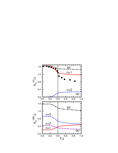
Figure 12: Kinetic energy terms (in units of $J$) per bond (13), as obtained for the $C$-AF phase of the cubic vanadates: high-spin $K_{1}^{(\gamma)}$ (solid lines) and low-spin $K_{2}^{(\gamma)}$ (dashed lines) and $K_{3}^{(\gamma)}$ (long-dashed lines), for increasing temperature $T/J$: (a) along the FM $c$ axis ($\gamma=c$); (b) within the AF $ab$ plane ($\gamma=ab$). In part (a) the experimental points from Ref. Miy03, for the low-energy spectral weight were reproduced, after proper rescaling to match the value of $K_{1}^{(\gamma)}$ at $T\to 0$. Parameters: $\eta=0.13$.

Table 6: Exchange constants $J_{\gamma}$ and optical spectral weights $K_{n}^{(\gamma)}$ (all in units of $J$) as obtained for: LaVO₃ ($C$-AF phase with $G$-type OO), and for YVO₃ ($G$-AF phase with $C$-type OO) at $T=0$ and above the magnetic transition at $T=0.85J$ ($\sim 300$ K). Parameters: $\eta=0.13$ and $T_{N}=140$ K.

		LaVO3		YVO3
		$C$-AF phase		$G$-AF phase
	$T$ (K)	$0$	$300$	$0$	$300$
	$J_{c}$	-0.107		0.224
	$J_{ab}$	0.171		0.171
	$K_{1}^{(c)}$	1.640	1.181	0.0	0.0
	$K_{2}^{(c)}$	0.0	0.280	0.586	0.494
	$K_{3}^{(c)}$	0.0	0.0	0.465	0.392
	$K_{1}^{(ab)}$	0.219	0.471	0.249	0.471
	$K_{2}^{(ab)}$	0.916	0.532	0.871	0.532
	$K_{3}^{(ab)}$	0.436	0.253	0.415	0.253

A crucial test of the present theory concerns the temperature dependence of the high-spin spectral weight along the $c$ axis $K_{1}^{(c)}$, which according to experiment decreases by about 50% between low temperature and $T=300$ K.Miy02 In the present theory based upon frozen OO this decrease amounts only to about 27% [Fig. 12(a)], and the maximal possible reduction of $K_{1}^{(c)}$ reached in the limit of $T\to\infty$ is by 33%. This result suggests that the frozen OO scenario in LaVO₃ is excluded by experiment; further arguments supporting this point of view are given in Sec. VI.3. Note also that the actual values of $K_{1}^{(c)}$, shown in Refs. Kha04, and Ole04, , had to be reduced to match the classical prediction at $T=0$.

A second classical state with $C$-type OO, as proposed for the low temperature $G$-AF phase of YVO₃,Bla01 gives an AF exchange constant along the $c$ axis,

$$J_{c}^{G-{\rm AF}}=\frac{1}{4}J(1-\eta r_{3}),$$ (120)

while the value of $J_{ab}^{G-{\rm AF}}$ is the same as $J_{ab}^{C-{\rm AF}}$, see Eq. (113), so in the present classical approach it does not change when the OO changes from the $G$-type to $C$-type. In contrast, depending on the type of OO, the exchange constant along the $c$ axis can be either FM or AF, as suggested by experimentMiy03 and confirmed by the data in Table 6. The actual values estimated with the same parameters as for LaVO₃ are: $J_{c}=9.0$ and $J_{ab}=6.8$ meV. Here one finds that $J_{c}>J_{ab}$ as in experiment, but the agreement with the experimental values,Ulr03 $J_{c}^{\rm exp}=3.1$ and $J_{ab}^{\rm exp}=2.6$ meV, is much poorer. Hence, we conclude that quantum effects beyond the present classical analysis such as orbital fluctuations,Kha01 orbital Peierls effect,Ulr03 ; Sir03 and spin-orbit coupling, Hor03 play here an important role and have to be included in a quantitative theory.

Furthermore, while the weights in the $ab$ planes are given by spin-spin correlations $s_{ab}$, as in Eqs. (117)–(119), for the spectral weights in the $C$-type OO one finds along the $c$ axis

$$K_{1}^{(c)} = 0,$$ (121)

$$K_{2}^{(c)} = \frac{1}{4}J\big{(}1-s_{c}\big{)},$$ (122)

$$K_{3}^{(c)} = \frac{1}{4}Jr_{3}\big{(}1-s_{c}\big{)}.$$ (123)

We evaluated these spectral weights (see Table 6) for the standard value of $\eta=0.13$ and for the spin-spin correlation function $s_{c}$ determined within the Oguchi method for an AF bond along the $c$ axis (Appendix C), stabilized by the above value of the AF interaction $J_{c}$, and taking again $T_{N}=0.4J$. It is along this axis where the theory predicts a markedly different behavior of the spectral weights from that found above for $G$-type OO, see Table 6. In spite of AF bonds in all three directions, the spectral weight distribution is again anisotropic — the weights are considerably higher for the $ab$ planes due to the broken cubic symmetry in orbital space. In addition, the spectral weights obtained in $ab$ planes at low temperature differ between the two AF phases, as the MF terms are larger in $G$-AF phase and make this case somewhat closer to the classical limit of $s_{ab}=-1$. Particularly the prediction that $K_{1}^{(c)}=0$, following from the classical $C$-type OO, is easy to verify. In fact, the experimental data are puzzling as one finds instead finite and temperature dependent spectral weight also for the low-energy regime in the $G$-AF phase of YVO₃,Miy02 ; Tsv04 pointing out once again that the present calculation with frozen OO is oversimplified.

VI.3 Composite spin-orbital dynamics in LaVO₃

Finally, we demonstrate that the scenario of strong JT interaction, quenching the orbital dynamics, cannot apply to LaVO₃. We do so by investigating its consequences for the orbital transition temperature $T_{\rm o}$ and for the temperature dependence of the optical intensity $K_{1}^{(c)}$ of the lowest multiplet transition. Consider first the transition temperature $T_{\rm o}$ associated with the phase transtion into the state with OO. We have already seen in Secs. III and IV that strong orbital-lattice coupling in a perovskite structure would in fact necessarily decouple orbital and spin degrees of freedom and lead to $T_{\rm o}\gg T_{N}$, contradicting the experiment.Miy02

The JT coupling between the JT-active local lattice modes $Q_{i}$ and the pseudospin (orbital) variables $\tau_{i}^{z}$ (which refer to the active $\{|a\rangle,|b\rangle\}$ orbitals along the $c$ axis) may be written as follows,

$${\cal H}_{\rm JT}=g\sum_{i}Q_{i}\tau_{i}^{z}+\frac{1}{2}\sum_{i}Q_{i}^{2},$$ (124)

where $Q_{i}$ is the appropriate linear combination of coordinates of the ligand ions next to site $i$. The above local coupling induces local distortions and an associated energy gain of $E_{\rm JT}=g^{2}/8$ (the JT energy) per site, and moreover generates a cooperative JT effect in the following way. As the oxygens are shared by two neighboring vanadium ions in the perovskite structure of LaVO₃, the JT distortions $Q_{i}$ at nearest-neighbor sites are not independent from each other. Hence the electron densities in $|a\rangle/|b\rangle$ orbitals at two vanadium ions at sites $i$ and $j$ in the $ab$ plane (see inset in Fig. 13) get coupled to each other, basically because they depend on the actual displacement $\delta$ of the shared oxygen ion. More specifically, this displacement generates interactions between the orbitalsKug82 ; Geh75 and one finds, taking care of the orthogonality constraint on the $Q_{i}$ variables,

$$H_{ab}(ij)=J_{\rm JT}\>\tau_{i}^{z}\tau_{j}^{z},$$ (125)

with the interaction constant being given by $J_{\rm JT}=2\lambda E_{\rm JT}=\frac{1}{4}\lambda g^{2}$. Here the coefficient $\lambda$ is determined by the phonon spectrum, viz. by all branches in which the local coordinates $Q_{i}$ participate, Geh75 and $\lambda<1$ (see e.g. Refs. Hal71, and Mil96, for how to estimate $\lambda$ for the perovskite lattice). The JT interaction (125) reflects the cooperative nature of the JT problem. It favors orbital alternation and thus supports the superexchange orbital interaction $J_{ab}^{\tau}$,Kha04 and the orbital model relevant for the $C$-AF phase of LaVO₃ is then

$${\cal H}_{\tau}=J_{c}^{\tau}\sum_{{\langle ij\rangle}\parallel c}\Big{(}{\vec{\tau}}_{i}\cdot{\vec{\tau}}_{j}-\frac{1}{4}\Big{)}+V_{ab}\sum_{{\langle ij\rangle}\parallel{ab}}\tau_{i}^{z}\tau_{j}^{z},$$ (126)

with $V_{ab}=J_{ab}^{\tau}+J_{\rm JT}$. The first term follows from the spin-orbital model, and $J_{c}^{\tau}=Jr_{1}$.

While the superexchange contribution to $V_{ab}$ is small (adopting the values of Ref. Mot03, , $J_{ab}^{\tau}\simeq 2$ meV, i.e., $J_{ab}^{\tau}\ll J_{c}^{\tau}\simeq 33$ meV), one finds that yet $V_{ab}>J_{c}^{\tau}$ if one assumes $\lambda=1$, i.e. if one basically identifies the JT interaction with the JT energy, and further accepts the estimate for $E_{\rm JT}\sim 27$ meV given in Ref. Mot03, . Then the Ising term quenches the $J_{c}^{\tau}$-driven orbital dynamics and leads to a cooperative transition at $T_{\rm o}$ which locks the orbitals in all three directions. However, one should be aware that the total energy decrease produced by the JT distortion of the lattice, $E^{\prime}_{\rm JT}$, as obtained in an ab initio calculation such as in Ref. Mot03, , actually equals $E^{\prime}_{\rm JT}=E_{\rm JT}+E_{\rm JT}^{\rm o}$, i.e. it comprises both the local energy gain $E_{\rm JT}$, which does not contribute to the ordering,Geh75 as well as the JT ordering energy $E_{\rm JT}^{\rm o}=z_{ab}J_{\rm JT}/8=\lambda E_{\rm JT}$. The JT contribution to $V_{ab}$ is therefore given by $J_{\rm JT}=2\lambda E^{\prime}_{\rm JT}/(1+\lambda)$, and since $\lambda$ is usually appreciably smaller than $1$ one should expect that $J_{\rm JT}$ is definitely smaller than $E^{\prime}_{\rm JT}$, so that it is more likely that actually $V_{ab}\lesssim J_{c}^{\tau}$.

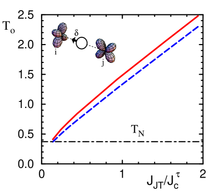
Figure 13: (Color online) Orbital transition temperature $T_{\rm o}$ for increasing JT interaction $J_{\rm JT}$ in: orbital-only model [Eq. (126), dashed line], and spin-orbital model [Eqs. (126) and (127), solid line], compared with the Néel temperature $T_{N}$ (dashed-dotted line). Both $T_{\rm o}$ and $T_{N}$ in units of $J_{c}^{\tau}$. The inset shows intersite orbital correlations due to JT distortions in LaVO₃.

To gain more insight in the role of the JT interaction we performed exact diagonalization of eight-site chains along the $c$ axis, combined with a MF treatment of the orbital interactions in the $ab$ plane, to determine the orbital transition temperature $T_{\rm o}$. As expected, it scales with $J_{\rm JT}$ in the regime of large JT interaction $J_{\rm JT}>0.1J_{c}^{\tau}$ (but still $J_{\rm JT}\lesssim 2J_{c}^{\tau}$) as shown in Fig. 13, as was also found in Ref. Mot03, . However, we were surprised to see that Motome et al.Mot03 have discarded this result considering it to be “an artefact of the MF treatment”, and argued that the coupling between neighboring sites is determined solely by $J_{c}^{\tau}$. The latter applies only in the limit of extremely anisotropic coupling, $V_{ab}\ll J_{c}^{\tau}$, which is not relevant here. In fact, it is a classical result Geh75 that the JT coupling of Eq. (124) also induces intersite interactions between the orbitals as in Eq. (125) which may actually dominate over the superexchange term and determine $T_{\rm o}$ in the limit of large $g$. As $T_{\rm o}$ is 20-80% above $T_{N}$ in other RVO₃ (R= Ce, Pr, Nd, Y, etc.) compounds,Miy03 it is not plausible that for R=La it is determined by superexchange alone. Therefore we argue that as the $ab$ plane correlations are of Ising-type, the MF result should be in fact a reasonable estimate for $T_{\rm o}$. Thus, the proximity of the orbital and the magnetic transitions in LaVO₃,Miy02 $T_{\rm o}\sim T_{N}$ ($\simeq 0.4J$), implies that the JT interaction is small, $J_{JT}\sim 0.1J_{c}^{\tau}$, and the JT splitting of the $xz/yz$-doublet is actually smaller than the superexchange energy scale itself, $\Delta_{\rm JT}=z_{ab}J_{\rm JT}/2=2J_{\rm JT}\sim 0.2J_{c}^{\tau}$.

Furthermore, as the spin and orbital exchange interactions are interrelated,Mot03 ; Kha04 spin disorder should reduce the effective orbital exchange $J_{c}^{\tau}$. Indeed, we have verified that this follows from the full spin-orbital superexchange modelKha01 which contains an extra term,

$${\cal H}_{s\tau}\!=\!\frac{1}{2}J_{c}^{\tau}\!\sum_{{\langle ij\rangle}\parallel c}\big{(}{\vec{S}}_{i}\cdot{\vec{S}}_{j}-1\big{)}\Big{[}\Big{(}1-\eta-\eta\frac{r_{3}}{r_{1}}\Big{)}\Big{(}{\vec{\tau}}_{i}\cdot{\vec{\tau}}_{j}+\frac{1}{4}\Big{)}-\eta\Big{]},$$ (127)

describing the coupling of spins and orbitals along the $c$ axis. However, $T_{\rm o}$ obtained from the complete spin-orbital model,

$${\cal H}_{U}(d^{2})\simeq{\cal H}_{\tau}+{\cal H}_{s\tau},$$ (128)

has about the same value as that found from ${\cal H}_{\tau}$ alone (see Fig. 13), and the estimate $\Delta_{\rm JT}\simeq 0.2J_{c}^{\tau}$ remains valid.

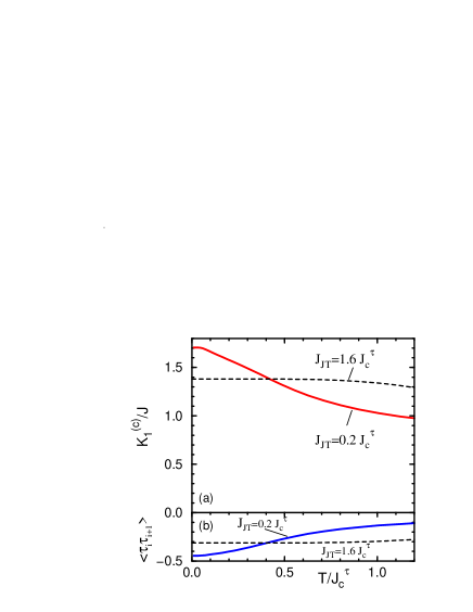
Figure 14: (Color online) Temperature dependence of: (a) optical spectral weight of the high-spin transition, $K_{1}^{(c)}$, in units of $J$ ($J$ is the principal energy scale of the spin-orbital model), and (b) orbital correlations $\langle\vec{\tau}_{i}\cdot\vec{\tau}_{i+1}\rangle$ along the $c$ axis (bottom), as obtained for — the spin-orbital model Eqs. (128), as given in Ref. Kha01, , with small $J_{JT}=0.2J_{c}^{\tau}$ (solid lines), and — the orbital model Eq. (126) with $J_{JT}=1.6J_{c}^{\tau}$, as analyzed in Ref. Mot03, (dashed lines).

Moreover, one finds that for large $J_{\rm JT}$ (e.g., $J_{\rm JT}=2E^{\prime}_{\rm JT}=54$ meV, i.e. for $\lambda=1$ and $E^{\prime}_{\rm JT}=27$ meV $\simeq 0.8J_{c}^{\tau}$, following Ref. Mot03, ) the temperature dependence of the optical intensity $K_{1}^{(c)}$ derived from ${\cal H}_{\tau}$ is weak below 300 K (Fig. 14), so adding orbital correlations in this range of parameters to the spin correlations of Sec. VI.2 cannot improve the agreement with experiment. Hence, this analysis clearly shows that: (i) a substantial variation of $K_{1}^{(c)}$ below 300K ($\sim J$, see Fig. 14) observed in Ref. Miy02, is obtained only for small $J_{\rm JT}$; (ii) while neither spin correlations for frozen OO, nor orbital correlations that follow from ${\cal H}_{\tau}$ alone would suffice, only the full spin-orbital model (128) that includes coupled spin-orbital fluctuations is able to explain a large enhancement of $K_{1}^{(c)}$ at low temperature. This was indeed demonstrated in Ref. Kha04, , where spin and orbital correlations were treated self-consistently, and only then the strong temperature dependence of $K_{1}^{(c)}$ could be successfully reproduced by the theory.

Summarizing, on comparing the results of Figs. 13 and 14 with the experimental data,Miy02 one has to conclude that the proximity of $T_{\rm o}$ and $T_{N}$ in LaVO₃ implies that $J_{\rm JT}$ is in fact much smaller than the total energy associated with the cooperative JT distortion $E^{\prime}_{\rm JT}\simeq 27$ meV estimated in Ref. Mot03, . The enhanced optical conductivity along the $c$ axis Miy02 also suggests that the local splitting $\Delta_{\rm JT}$ is smaller than the dynamical orbital exchange $J_{c}^{\tau}$, thus supporting the scenario of fluctuating orbitalsKha01 in LaVO₃. Therefore, the assumption of rigid OO, which was so successful for LaMnO₃, fails for LaVO₃ and the full quantum spin-orbital many-body problem has to be treated explicitly.Kha04

VII Summary and conclusions

The main purpose of this paper was to make the experimental consequences of the superexchange spin-orbital models for correlated transition metal oxides with orbital degeneracy more transparent. We formulated a general approach to the spectral weights in optical spectroscopy and illustrated it on several examples with different multiplet structure. While a general feature of all the superexchange spin-orbital models is a tendency towards enhanced quantum fluctuations,Fei97 ; Kha00 we gave reasons why in many situations such fluctuations are quenched. One then arrives at much simpler reduced models, where certain states with OO allow for a good insight into the mechanisms responsible for the magnetic interactions and for the optical spectral weights. The common feature of all these cases is that the knowledge of only a few effective parameters, the superexchange energy $J$, Hund’s exchange $\eta$ and the charge-transfer parameter $R$, is sufficient to work out the quantitative predictions of the theory for a given type of orbital ordered state. In some of these cases the theoretical models simplify so much that it is even possible to perform calculations with the help of a pocket calculator.

The cases of copper fluoride KCuF₃ and the manganite LaMnO₃ turned out to be simpler, and could be understood with frozen OO and quenched orbital dynamics below the structural transitions which occur at much higher temperatures than the Néel temperature, $T_{s}\gg T_{N}$. However, we have also seen that particularly in $t_{2g}$ systems, in the cubic titanates and vanadates, the orbital dynamics may not be quenched. Therefore, in some cases only the full quantum many-body problem gives proper answers for the experimental situation.

We came to these conclusions by analyzing in detail the consequences of decoupling of the spin and orbital degrees in states with rigid OO and by comparing the predictions of the theory with the experimental data, wherever available. In the undoped manganite LaMnO₃ we could provide a consistent explanation of the magnetic and optical experimental data by deducing the values of the above effective parameters $\{J,\eta,R\}$, and next showing that both the magnetic exchange constants $J_{ab}$ and $J_{c}$, and the anisotropy and the temperature dependence of the low-energy optical spectral weights can be reproduced by the theory in a satisfactory way. In the case of the copper fluoride KCuF₃ optical data were not available, but the constraints in the theory given by the exchange constants are so strong that we could conclude that the insulating state in this compound has charge-transfer character. It remains to be verified by future experiments to what extent the predictions made here concerning the optical spectral weights and based on the classical picture with ordered $e_{g}$ orbitals apply to KCuF₃.

Also for LaTiO₃ and YTiO₃ we investigated the classical states with OO given by certain wavefunctions which guarantee that the observed isotropic AF or FM states are realized. As in all other cases, the theory predicts in such states a rather pronounced temperature dependence and spectral weight transfers in the optical spectra near the magnetic transition. Future experiments will have to establish whether and to what extent such a scenario relaying on rigid OO could be valid. However, already without these data we could demonstrate, by looking at the exchange constants, that there are certain indications that orbital fluctuations play a role and thus the quantum physics might dominate here over the thermal fluctuations of the spins alone.

Table 7: Values of the effective parameters of spin-orbital models: superexchange $J$ (in meV), Hund’s parameter $\eta$, the CT parameter $R$, and the microscopic parameters consistent with these effective parameters: intraorbital Coulomb interaction $U$, Hund’s exchange $J_{H}$, and the energy of the lowest CT excitation $\Delta$ (all in eV), deduced from the present analysis of the magnetic and optical properties of representative transition metal compounds with perovskite structure. The values of $J_{H}$ and $U$ in case of LaVO₃ and LaMnO₃ were obtained from the optical spectra, while the ones for KCuF₃ are the same as in Ref. Lic95, .

		LaVO3	LaMnO3	KCuF3
parameters	orbitals	$t_{2g}$	$e_{g}$	$e_{g}$
effective	$J$	40	150	33
	$\eta$	0.13	0.18	0.12
	$R$	$<0.4$	0.6	1.2
microscopic	$U$	3.8	3.8	7.5
	$J_{H}$	0.50	0.67	0.90
	$\Delta$	$>5.0$	3.5	4.0

The case of the cubic vanadate LaVO₃ really shows that one may encounter the full complexity of the spin-orbital superexchange model when the spins and orbitals fluctuate coherently, and these fluctuations are essential to get a meaningful quantitative description of the optical data. This case in particular demonstrates the importance of combining the magnetic and optical data. Whereas the classical analysis of the spin fluctuations for frozen orbitals seems to suffice to explain the exchange constants in LaVO₃, by looking at the optics one realizes that the picture of frozen OO induced by large JT coupling is here misleading, and the complete spin-orbital dynamics has to be considered instead.

Before concluding this paper, we summarize in Table 7 the effective parameters of the spin-orbital models,notepa and the possible values of the microscopic parameters — the Coulomb interaction $U$, Hund’s exchange $J_{H}$, and the charge transfer energy $\Delta$, that are consistent with these effective parameters. The values of the superexchange constant are $33<J<40$ meV for KCuF₃ and LaVO₃, while for LaMnO₃ the value of this parameter is much higher, $J\sim 140$ meV. This difference reflects a rather high value of the effective hopping parameter $t$ in the undoped manganite. By considering the optical data of LaVO₃ and LaMnO₃ we came to the conclusion that Hund’s exchange $J_{H}$ is somewhat reduced from the respective atomic values,Zaa90 and we give already these reduced parameters in Table 7, accompanied by the corresponding values of $U$.

Summarizing, we have illustrated a common approach to the optical and the magnetic data in Mott insulators with orbital degeneracy, which provides the basis for a better theoretical understanding of the experimental constraints on the underlying phenomena and on the model parameters. It is a unique feature of these systems that the superexchange interactions, and the spin, orbital, and composite spin-and-orbital correlations induced by them, are responsible for the distribution of spectral weight in the optical excitations. We hope that extending the present analysis of the high-energy excitations in the upper Hubbard band by an analysis of the low-energy excitations that occur in doped systems, will allow to develop a quantitative theoretical approach designed to describe the optical spectra of doped transition metal insulators.

Appendix A Effective model for LaMnO₃

Here we present an analysis of the magnetic and optical data within an effective $d-d$ model for LaMnO₃, given by the ${\cal H}_{U}(d^{4})$ term alone, i.e., assuming $R=0$ in Eq. (56). Unlike in KCuF₃, the alternating OO in LaMnO₃ refers to the orbitals occupied by electrons, and is characterized by a single angle $\theta$ in Eqs. (III.2). We performed an analysis of the exchange constants $J_{c}$ (69) and $J_{ab}$ (68) as functions of the effective parameters $J$ and $\eta$. Although these parameters cannot be uniquely determined, we have verified that only a narrow range of the orbital angle $\theta\sim 90^{\circ}-100^{\circ}$ gives reasonable agreement with experiment. Here we present the results obtained with $J=170$ meV and $\eta=0.16$.

Both exchange constants exhibit a rather strong dependence on the orbital angle $\theta$ (Fig. 15). In contrast to the case of KCuF₃, the effective model parameters obtained at $R=0$ suffices to explain even almost quantitatively the observed exchange constants in LaMnO₃. This result is also consistentnotetg with the earlier analysis of Ref. Fei99, . Due to the strong dependence of the exchange constants $J_{ab}$ and $J_{c}$ on the angle $\theta$, one can exclude the OO of alternating directional $(3x^{2}-r^{2})/(3y^{2}-r^{2})$ orbitals, obtained with $\theta=120^{\circ}$ in Eqs. (III.2).

While it is frequently assumed that the $t_{2g}$ superexchange (66) is large, the present analysis shows that a consistent description of the magnetic properties requires instead a rather moderate value of $J_{t}$ in LaMnO₃. For the present parameters one finds $J_{t}=1.70$ meV,notes2 and $J_{t}$ increases by $\sim 35$% when the CT terms are included (see Sec. IV.3). Although it might be argued that $J_{t}\sim 2$ meV is too large as the experimental value of $T_{N}$ in CaMnO₃ is only 110 K, Wol55 one deals here de facto with different values of the $U$, $J_{H}$ and $\Delta$ parameters, namely with those for Mn²⁺ ions instead of the ones for Mn³⁺ ions, which apply in the intermediate excited states contributing to the superexchange in CaMnO₃. Yet the differences in these parameter values cannot be large from the very nature of their physical origin, and so $J_{t}$ for LaMnO₃ cannot differ by more than a factor of 2 from the value of the $t_{2g}$-induced superexchange in CaMnO₃.Fei99 This supports our finding that a small ratio $J_{t}\sim 4\times 10^{-3}t$ corresponds to realistic parameter values for LaMnO₃.

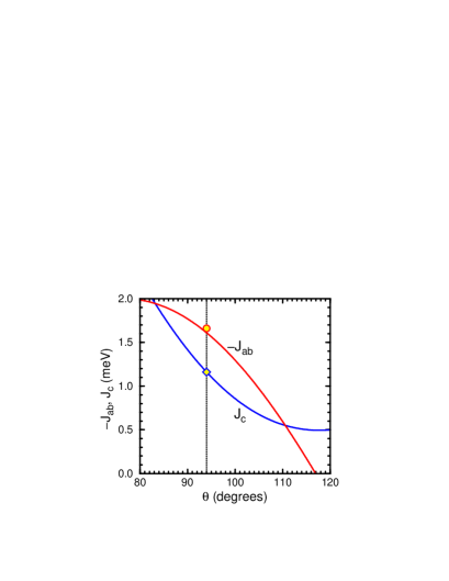
Figure 15: (Color online) Superexchange interactions $-J_{ab}$ (68) and $J_{c}$ (69) as functions of the orbital angle $\theta$ (solid lines), obtained within the effective superexchange model ${\cal H}_{U}(d^{4})$ ($R=0$). Experimental valuesMou96 of $-J_{ab}$ and $J_{c}$ for LaMnO₃ (indicated by circle and diamond) are nearly reproduced for the OO with $\theta=94^{\circ}$. Parameters: $J=170$ meV, $\eta=0.16$.

Next we consider the temperature dependence of the spin-spin correlations and the optical spectral weights (15). As in the full model discussed in Sec. IV.4, one may assume frozen OO in the relevant temperature range below room temperature, and derive the temperature dependence of the optical spectral weights from that of the intersite spin-spin correlations (12), with the latter determined in a cluster method as explained in Appendix B. Using the exchange interactions obtained with the present parameters at $\theta=94^{\circ}$ (Fig. 15), one finds the empirical estimateFle04 $T_{N}\simeq 146$ K, which reasonably agrees with the experimental value $T_{N}^{\rm exp}=136$ K.Mou96 The AF bonds feel staggered MF terms for $T<T_{N}$, so the spin-spin correlations $s_{c}$ had to be determined by a numerical solution, as explained in Appendix B. Both correlation functions change fast close to $T_{N}$, reflecting the temperature dependence of the Brillouin function, and remain finite at $T\gg T_{N}$ [Fig. 16(a)].

Figure 16: (Color online) Temperature dependence of: (a) spin-spin correlations $\langle\vec{S}_{i}\cdot\vec{S}_{j}\rangle_{\gamma}$ for $\gamma=a,c$, and the order parameter $\langle S^{z}\rangle$ (dashed line); (b) kinetic energies $K_{1}^{(\gamma)}$ for the high-spin excitations, standing for the optical intensities (15) at low energy along $\gamma=a,c$ axes (solid lines), and total kinetic energies $K^{(\gamma)}$ (long-dashed lines), as obtained for LaMnO₃ within the effective superexchange model ${\cal H}_{U}(d^{4})$ for the OO given by an angle $\theta\simeq 94^{\circ}$. Parameters as in Fig. 15.

The effective model also allows one to discuss the qualitative features of the spectral weight distribution in the optical spectra. The theory predicts that only high-spin optical excitations are allowed at $T=0$ for the FM bonds in the $ab$ planes, and one finds for this polarization a large kinetic energy $K_{1}^{(ab)}$ [Fig. 16(b)]. In contrast, the optical excitations for the AF bonds along the $c$ axis are predominantly of low-spin character, and thus the kinetic energy $K_{1}^{(c)}$ is rather small, resulting in a large anisotropy $K_{1}^{(ab)}:K_{1}^{(c)}\sim 10:1$ of the low-energy optical intensities confirmed by experiment.Kov04 When the temperature increases and the spin-spin correlations weaken, this anisotropy is reduced, but remains pronounced also at $T>T_{N}$ and still exceeds $2:1$ at $T=300$ K due to the persisting OO. As shown elsewhere,Ole04 also a quantitative analysis of the present effective model gives a rather satisfactory agreement with the optical dataKov04 in the entire temperature range. In contrast, the total optical intensities have a much weaker temperature dependence and anisotropy [Fig. 16(b)]. Thus, the main features on the experimentally observed intensity distribution and its temperature variation in the optical spectraKov04 are well reproduced already by the present effective model.

Finally, we verify whether the used parameters $J=170$ meV and $\eta=0.16$ could be derived from the microscopic parameters of the CT model. The value of $J_{H}=0.90$ eV follows from the spectroscopic values of the $B$ and $C$ Racah parameters,Boc92 so $\eta=0.16$ implies $U\simeq 5.6$ eV. Knowing the value of $J$, this leads to an estimated effective $d-d$ hopping element $t\simeq 0.49$ eV. Indeed, one finds that these microscopic parameters are in the expected range. The effective Coulomb interaction was estimated within the effective $d-d$ model for LaMnO₃ as $U\sim 5.5$ eV from spectroscopic data, Miz96 so the agreement is close to perfect. Furthermore, taking the usually accepted values of $t_{pd}=1.5$ eV and $\Delta=5.0$ eV, following Refs. Boc92, and Miz96, , one finds a very plausible value of the effective hopping parameter $t=t_{pd}^{2}/\Delta=0.45$ eV, again quite close to the value derived above. Note that the experimental magnetic interactions in doped bilayer manganites were explained with a similar value of $t=0.48$ eV fixed by experiment.Ole03 This favorable comparison emphasizes once again our main conclusion that the relevant model parameters can be derived by combining the results of magnetic and optical experiments, whenever available.

Appendix B Spin-spin correlations in LaMnO₃

Here we describe briefly a simple method which we used to determine the spin-spin correlation functions $s_{ab}$ and $s_{c}$ for a pair of interacting spins $S=2$ at nearest neighbor Mn ions in LaMnO₃. The spin-spin correlations were obtained by performing a statistical average over the exact eigenstates for a single (FM or AF) bond, found in the presence of MF terms acting at each spin of the bond and originating from its neighboring spins. This, in fact, is the simplest cluster MF theory, known in the theory of magnetism as the Oguchi method.Ogu60 As long as the MF terms vanish (at $T>T_{N}$), one finds for the various eigenstates with degeneracy $(2S_{\rm tot}+1)$, labeled by the total spin $S_{\rm tot}=0,1,\cdots,4$,

$$\langle S_{\rm tot}|{\vec{S}}_{i}\cdot{\vec{S}}_{j}|S_{\rm tot}\rangle=\frac{1}{2}S_{\rm tot}(S_{\rm tot}+1)-6.$$ (129)

Depending on $S_{\rm tot}$ the scalar product $\langle S_{\rm tot}|{\vec{S}}_{i}\cdot{\vec{S}}_{j}|S_{\rm tot}\rangle$ varies between $-6$ and $4$.

Consider first a FM bond $\langle ij\rangle$ in the $ab$ plane, with the Hamiltonian given by,

$$H_{ij}^{(ab)}=-|J_{ab}|{\vec{S}}_{i}\cdot{\vec{S}}_{j}-h_{ab}(S_{i}^{z}+S_{j}^{z}),$$ (130)

where for the $A$-AF phase with uniform order parameter in the $ab$ plane $\langle S^{z}\rangle=\langle S^{z}_{i}\rangle$ the identical MF acting at both spins is

$$h_{ab}=(3|J_{ab}|+2J_{c})\langle S^{z}\rangle.$$ (131)

At $T>T_{N}$ the eigenenergies of $H_{ij}^{(ab)}$ follow from Eq. (129). For $T<T_{N}$ the order parameter $\langle S^{z}\rangle$ could in principle be determined self-consistently in the present cluster approach. However, to gain a qualitative insight into the temperature dependence of $s_{ab}$ it suffices to use a self-consistent solution of the MF equation,

$$\langle S^{z}\rangle = \frac{2S+1}{2}\coth\Big{(}\frac{2S+1}{2}\frac{T_{N}}{2T}\langle S^{z}\rangle\Big{)}$$ (132)

$$- \frac{1}{2}\coth\Big{(}\frac{1}{2}\frac{T_{N}}{2T}\langle S^{z}\rangle\Big{)}.$$

As the MF value $k_{\rm B}T_{N}^{\rm MF}=4(2|J_{ab}|+J_{c})$ is overestimated, it is appropriate to use in Eq. (132) the value of $T_{N}$ after an empirical reduction,Fle04 leading to $T_{N}\simeq 0.705T_{N}^{\rm MF}$. One finds an analytic solution for $s_{ab}$:

$$s_{ab}=\frac{4z_{4}-3z_{2}-5z_{1}-6z_{0}}{z_{4}+z_{3}+z_{2}+z_{1}+z_{0}},$$ (133)

where the terms $z_{i}$ refer to the subspaces of total spin $S_{\rm tot}$,

$$z_{4} = 1+2\cosh x+2\cosh 2x+2\cosh 3x$$ (134)

$$+ 2\cosh 4x,$$

$$z_{3} = (1+2\cosh x+2\cosh 2x+2\cosh 3x)$$ (135)

$$\times \exp(-4\beta|J_{ab}|),$$

$$z_{2} = (1+2\cosh x+2\cosh 2x)\exp(-7\beta|J_{ab}|),$$ (136)

$$z_{1} = (1+2\cosh x)\exp(-9\beta|J_{ab}|),$$ (137)

$$z_{0} = \exp(-10\beta|J_{ab}|),$$ (138)

with $x=\beta h_{ab}$ and $\beta=1/k_{\rm B}T$. Note that the term $\propto z_{3}$ is absent in the numerator of Eq. (133), because $\langle S_{\rm tot}=3|{\vec{S}}_{i}\cdot{\vec{S}}_{j}|S_{\rm tot}=3\rangle=0$ [see Eq. (129)].

For an AF bond $\langle ij\rangle$ along the $c$ axis the Hamiltonian is given by

$$H_{ij}^{(c)}=J_{c}{\vec{S}}_{i}\cdot{\vec{S}}_{j}-h_{c}(S_{i}^{z}-S_{j}^{z}),$$ (139)

where the molecular field

$$h_{c}=(4|J_{ab}|+J_{c})\langle S^{z}\rangle.$$ (140)

alternates between the sites $i$ and $j$, so $\langle S^{z}_{i}\rangle=-\langle S^{z}_{j}\rangle=\langle S^{z}\rangle$. Unlike for the FM bond, the field $h_{c}$ couples now states which belong to different values of $S_{\rm tot}$ (but to the same value of $S_{\rm tot}^{z}$). The staggered MF plays no role for $S_{\rm tot}^{z}=4$, while for $S_{\rm tot}^{z}<4$ the eigenstates have been found by diagonalizing the matrices, with diagonal elements following from Eq. (129), and offdiagonal ones $\propto h_{c}$:

— for $S_{\rm tot}^{z}=3$,

$$\left(\begin{array}[]{ccc}4J_{c}&-h_{c}\\[5.69046pt] -h_{c}&0\end{array}\right),$$ (141)

— for $S_{\rm tot}^{z}=2$,

$$\textstyle{\left(\begin{array}[]{ccc}4J_{c}&-2\sqrt{\frac{3}{7}}\;h_{c}&0\\[5.69046pt] -2\sqrt{\frac{3}{7}}\;h_{c}&0&-4\sqrt{\frac{1}{7}}\;h_{c}\\[5.69046pt] 0&-4\sqrt{\frac{1}{7}\;}h_{c}&-3J_{c}\end{array}\right),}$$ (142)

— for $S_{\rm tot}^{z}=1$,

$$\textstyle{\left(\begin{array}[]{cccc}4J_{c}&-\sqrt{\frac{15}{7}}\;h_{c}&0&0\\[5.69046pt] -\sqrt{\frac{15}{7}}\;h_{c}&0&-\frac{16}{\sqrt{70}}\;h_{c}&0\\[5.69046pt] 0&-\frac{16}{\sqrt{70}}\;h_{c}&-3J_{c}&-\sqrt{\frac{21}{5}}\;h_{c}\\[5.69046pt] 0&0&-\sqrt{\frac{21}{5}}\;h_{c}&-5J_{c}\end{array}\right),}$$ (143)

— for $S_{\rm tot}^{z}=0$,

$$\textstyle{\left(\begin{array}[]{ccccc}4J_{c}&-\frac{4}{\sqrt{7}}h_{c}&0&0&0\\[5.69046pt] -\frac{4}{\sqrt{7}}h_{c}&-\lambda&-\frac{12}{\sqrt{35}}h_{c}&0&0\\[5.69046pt] 0&-\frac{12}{\sqrt{35}}h_{c}&-3J_{c}&-2\sqrt{\frac{7}{5}}h_{c}&0\\[5.69046pt] 0&0&-2\sqrt{\frac{7}{5}}h_{c}&-5J_{c}&-2\sqrt{2}h_{c}\\[5.69046pt] 0&0&0&-2\sqrt{2}h_{c}&-6J_{c}\\[5.69046pt] \end{array}\right).}$$ (144)

In this way a complete set of eigenstates $\{|n\rangle\}$ with energies $\{E_{n}\}$ for $n=1,2,\cdots,25$ was determined. Finally, the spin-spin correlation function $s_{c}$ was found using a standard formula

$$s_{c}=\frac{1}{Z}\sum_{n}\langle n|{\vec{S}}_{i}\cdot{\vec{S}}_{j}|n\rangle\exp(-\beta E_{n}),$$ (145)

where $Z=\sum_{n}\exp(-\beta E_{n})$ is the partition function.

Appendix C Spin-spin correlations in LaVO₃ and in YVO₃

The short-range spin-spin correlations $s_{\gamma}$ for the cubic vanadates were determined using the Oguchi methodOgu60 for a bond of interacting $S=1$ spins. As in the case of LaMnO₃ (see Appendix B), we solve exactly a single FM (AF) bond $\langle ij\rangle$ with interaction $J_{c}$ ($J_{ab}$), and the MF terms $\propto\langle S^{z}\rangle$ originating from neighboring spins and acting on each spin of the bond. In the present case the scalar product is given by

$$\langle S_{\rm tot}|{\vec{S}}_{i}\cdot{\vec{S}}_{j}|S_{\rm tot}\rangle=\frac{1}{2}S_{\rm tot}(S_{\rm tot}+1)-2.$$ (146)

For a FM bond, now along the $c$ axis, one finds an analytic solution. Kha04 This problem is analogous to that given by Eq. (131). Using the MF approximation, the order parameter $\langle S^{z}\rangle$ was determined from Eq. (132) with $S=1$, and $T_{N}^{\rm MF}=4(2J_{ab}+|J_{c}|)/3$ was reduced to $T_{N}\simeq 0.684T_{N}^{\rm MF}$ as appropriate for $S=1$ spins.Fle04 The final result for $s_{c}$ reads

$$s_{c}=\frac{z_{2}-z_{1}-2z_{0}}{z_{2}+z_{1}+z_{0}},$$ (147)

where the terms $z_{i}$ originate from different subspaces of total spin $S_{\rm tot}=2,1,0$,

$$z_{2} = 1+2\cosh x+2\cosh 2x,$$ (148)

$$z_{1} = (1+2\cosh x)\exp(-2\beta|J_{c}|),$$ (149)

$$z_{0} = \exp(-3\beta|J_{c}|).$$ (150)

Here

$$h_{c}=(4J_{ab}+|J_{c}|)\langle S^{z}\rangle,$$ (151)

$x=\beta h_{c}$ and $\beta=1/k_{\rm B}T$; compare with Eq. (140).

For an AF bond $\langle ij\rangle$ in the $ab$ plane the MF Hamiltonian is given by

$$H_{ij}^{(ab)}=J_{ab}{\vec{S}}_{i}\cdot{\vec{S}}_{j}-h_{ab}(S_{i}^{z}-S_{j}^{z}),$$ (152)

In analogy to an AF bond in LaMnO₃ (see Appendix B), the correlation function $s_{ab}$ can be found numerically by considering the subspaces of $S_{\rm tot}^{z}$. The molecular field,

$$h_{ab}=(3J_{ab}+2|J_{c}|)\langle S^{z}\rangle,$$ (153)

does not contribute to the highest eigenenergies $E_{8,9}=J_{ab}$ in the subspace of $S_{\rm tot}^{z}=2$ [cf. with Eq. (131)], while the remaining eigenstates had to be found by diagonalizing the matrices corresponding to other values of $S_{\rm tot}^{z}$:

— for $S_{\rm tot}^{z}=1$,

$$\left(\begin{array}[]{cc}J_{ab}&-h_{ab}\\[5.69046pt] -h_{ab}&-J_{ab}\end{array}\right),$$ (154)

— for $S_{\rm tot}^{z}=0$,

$$\textstyle{\left(\begin{array}[]{ccc}J_{ab}&-\frac{2}{\sqrt{3}}\;h_{ab}&0\\[5.69046pt] -\frac{2}{\sqrt{3}}\;h_{ab}&-J_{ab}&-2\sqrt{\frac{2}{3}}\;h_{ab}\\[5.69046pt] 0&-2\sqrt{\frac{2}{3}}\;h_{ab}&-2J_{ab}\end{array}\right).}$$ (155)

By solving the above eigenproblems, we determined a complete set of eigenstates $\{|n\rangle\}$, with energies $E_{n}$, labeled by $n=1,2,\cdots,9$. Therefore, the spin-spin correlation function $s_{ab}$ for two interactings $S=1$ spins on an AF bond follows in the present case from an equation similar to Eq. (145), with the relevant matrix elements $\langle n|{\vec{S}}_{i}\cdot{\vec{S}}_{j}|n\rangle$ now given by Eq. (146).

References

- (1) M. Imada, A. Fujimori, and Y. Tokura, Rev. Mod. Phys. 70, 1039 (1998).
- (2) E. Dagotto, T. Hotta, and A. Moreo, Phys. Rep. 344, 1 (2001); E. Dagotto, New J. Phys. 7, 67 (2005).
- (3) E. Dagotto, Nanoscale Phase Separation and Colossal Magnetoresistance, Springer Series in Solid State Sciences Vol. 136 (Springer-Verlag, Heidelberg, 2003).
- (4) S. Maekawa, T. Tohyama, S. E. Barnes, S. Ishihara, W. Koshibae, and G. Khaliullin, Physics of Transition Metal Oxides, Springer Series in Solid State Sciences Vol. 144 (Springer-Verlag, Heidelberg, 2004).
- (5) Y. Tokura and N. Nagaosa, Science 288, 462 (2000); Y. Tokura, Physics Today, July 2003, p. 50.
- (6) P. W. Anderson, Phys. Rev. 115, 2 (1959).
- (7) K. I. Kugel and D. I. Khomskii, Usp. Fiz. Nauk 136, 621 (1982) [Sov. Phys. Usp. 25, 231 (1982)].
- (8) M. Cyrot and C. Lyon-Caen, J. Phys. (Paris) 36, 253 (1975); S. Inagaki, J. Phys. Soc. Jpn. 39, 596 (1975); C. Castellani, C. R. Natoli, and J. Ranninger, Phys. Rev. B18, 4945 (1978); 18, 4967 (1978); 18, 5001 (1978).
- (9) L. F. Feiner, A. M. Oleś, and J. Zaanen, Phys. Rev. Lett. 78, 2799 (1997).
- (10) G. Khaliullin and V. Oudovenko, Phys. Rev. B56, 14243(R) (1997); L. F. Feiner, A. M. Oleś, and J. Zaanen, J. Phys.: Condens. Matter 10, L555 (1998); G. Khaliullin and R. Kilian, ibid. 11, 9757 (1999).
- (11) A. M. Oleś, L. F. Feiner, and J. Zaanen, Phys. Rev. B61, 6257 (2000).
- (12) S. Ishihara, J. Inoue, and S. Maekawa, Phys. Rev. B55, 8280 (1997); R. Shiina, T. Nishitani, and H. Shiba, J. Phys. Soc. Jpn. 66, 3159 (1997).
- (13) L. F. Feiner and A. M. Oleś, Phys. Rev. B59, 3295 (1999).
- (14) A. Weisse and H. Fehske, New J. Phys. 6, 158 (2004).
- (15) G. Khaliullin and S. Maekawa, Phys. Rev. Lett. 85, 3950 (2000); G. Khaliullin, Phys. Rev. B64, 212405 (2001).
- (16) G. Khaliullin, P. Horsch, and A. M. Oleś, Phys. Rev. Lett. 86, 3879 (2001).
- (17) H. F. Pen, J. van den Brink, D. I. Khomskii, and G. A. Sawatzky, Phys. Rev. Lett. 78, 1323 (1997); R. Shiina, F. Mila, F.-C. Zhang, and T. M. Rice, Phys. Rev. B63, 144422 (2001); S. Di Matteo, N. B. Perkins, and C. R. Natoli, ibid. 65, 054413 (2002); S. Di Matteo, G. Jackeli, C. Lacroix, and N. B. Perkins, Phys. Rev. Lett. 93, 077208 (2004); S. Di Matteo, G. Jackeli, and N. B. Perkins, Phys. Rev. B72, 024431 (2005); Phys. Rev. B72, 020408(R) (2005).
- (18) A. M. Oleś, Acta Phys. Polon. B 32, 3303 (2001); Phys. Status Solidi (b) 236, 281 (2003); ibid. 242, 963(E) (2005).
- (19) P. Fazekas, Lecture Notes on Electron Correlation and Magnetism (World Scientific, Singapore, 1999).
- (20) G. Khaliullin, P. Horsch, and A. M. Oleś, Phys. Rev. B70, 195103 (2004).
- (21) J. S. Lee, M. W. Kim, and T. W. Noh, New J. Phys. 7, 147 (2005).
- (22) D. Baeriswyl, J. Carmelo, and A. Luther, Phys. Rev. B33, 7247 (1986).
- (23) P. Horsch and W. Stephan, Phys. Rev. B48, 10595 (1993); H. Eskes and A. M. Oleś, Phys. Rev. Lett. 73, 1279 (1994); H. Eskes, A. M. Oleś, M. Meinders, and W. Stephan, Phys. Rev. B50, 17980 (1994).
- (24) M. Aichhorn, P. Horsch, W. von der Linden, and M. Cuoco, Phys. Rev. B65, 201101(R) (2002).
- (25) J. Kanamori, J. Phys. Chem. Solids 10, 87 (1959).
- (26) Y. Motome, H. Seo, Z. Fang, and N. Nagaosa, Phys. Rev. Lett. 90, 146602 (2003).
- (27) K. Tobe, T. Kimura, Y. Ohimoto, and Y. Tokura, Phys. Rev. B64, 184421 (2001).
- (28) N. N. Kovaleva, A. V. Boris, C. Bernhard, A. Kulakov, A. Pimenov, A. M. Balbashov, G. Khaliullin, and B. Keimer, Phys. Rev. Lett. 93, 147204 (2004).
- (29) S. Miyasaka, Y. Okimoto, and Y. Tokura, J. Phys. Soc. Jpn. 71, 2086 (2002).
- (30) A. A. Tsvetkov, F. P. Mena, P. H. M. van Loosdrecht, D. van der Marel, Y. Ren, A. A. Nugroho, A. A. Menovsky, I. S. Elfimov, and G. A. Sawatzky, Phys. Rev. B69, 075110 (2004).
- (31) J. S. Lee, Y. S. Lee, T. W. Noh, S. J. Oh, J. Yu, S. Nakatsui, H. Fukazawa, and Y. Maeno, Phys. Rev. Lett. 89, 257402 (2002).
- (32) J. Zaanen, G. A. Sawatzky, and J. W. Allen, Phys. Rev. Lett. 55, 418 (1985).
- (33) We note, however, that frequently the average energy of a CT type excitation is considered instead and compared with .
- (34) J. B. Goodenough, Magnetism and the Chemical Bond (Interscience, New York, 1963).
- (35) J. Zaanen and A. M. Oleś, Phys. Rev. B37, 9423 (1988); H. Eskes and J. H. Jefferson, ibid. 48, 9788 (1993).
- (36) M. V. Mostovoy and D. I. Khomskii, Phys. Rev. Lett. 92, 167201 (2004).
- (37) O. K. Andersen, N. Klose, and H. Nohl, Phys. Rev. B17, 1209 (1978).
- (38) J. Zaanen and A. M. Oleś, Phys. Rev. B48, 7197 (1993).
- (39) J. S. Griffith, The Theory of Transition Metal Ions (Cambridge University Press, Cambridge, 1971).
- (40) A. M. Oleś, Phys. Rev. B28, 327 (1983).
- (41) Fractional contributions due to exchange terms shown in the spectrum for the case [see Fig. 1(a)] follow from the differences between the exchange elements in Hamiltonian (2) (see Table I), and were obtained using the relation satisfied approximately by the experimental values for Mn2+ ions.Zaa90
- (42) D. van der Marel and G. A. Sawatzky, Phys. Rev. B37, 10674 (1988).
- (43) T. Mizokawa and A. Fujimori, Phys. Rev. B54, 5368 (1996).
- (44) M. V. Mostovoy and D. I. Khomskii, Phys. Rev. Lett. 89, 227203 (2002); A. J. W. Reitsma, L. F. Feiner, and A. M. Oleś, New J. Phys. 7, 121 (2005).
- (45) P. F. Maldague, Phys. Rev. B16, 2437 (1977).
- (46) A. Chattopadhyay, A. J. Millis, and S. Das Sarma, Phys. Rev. B61, 10738 (2000).
- (47) K. H. Ahn and A. J. Millis, Phys. Rev. B61, 13545 (2000).
- (48) F. Mack and P. Horsch, Phys. Rev. Lett. 82, 3160 (1999).
- (49) S. Kadota, I. Yamada, S. Yoneyama, and K. Hirakawa, J. Phys. Soc. Jpn. 23, 751 (1967).
- (50) S. K. Satija, J. D. Axe, G. Shirane, H. Yoshizawa, and K. Hirokawa, Phys. Rev. B21, 2001 (1980).
- (51) L. Paolasini, R. Caciuffo, A. Sollier, P. Ghigna, and M. Altarelli, Phys. Rev. Lett. 88, 106403 (2002); R. Caciuffo, L. Paolasini, A. Sollier, P. Ghigna, E. Pavarini, J. van den Brink, and M. Altarelli, Phys. Rev. B65, 174425 (2002).
- (52) M. T. Hutchings, E. J. Samuelsen, G. Shirane, and K. Hirakawa, Phys. Rev. 188, 919 (1969).
- (53) De facto, the values of and differ and depend on bond direction below the structural transition when the JT distortions remove the degeneracy of the orbitals.Ole00 Here the idealized case of is discussed.
- (54) J. Zaanen and G. A. Sawatzky, J. Solid State Chem. 88, 8 (1990).
- (55) A. I. Lichtenstein, V. I. Anisimov, and J. Zaanen, Phys. Rev. B52, 5467(R) (1995).
- (56) J. E. Medvedeva, M. A. Korotin, V. I. Anisimov, and A. J. Freeman, Phys. Rev. B65, 172413 (2002).
- (57) D. A. Tennant, T. G. Perring, R. A. Cowley, and S. E. Nagler, Phys. Rev. Lett. 70, 4003 (1993); B. Lake, D. A. Tennant, and S. E. Nagler, ibid. 85, 832 (2000); D. A. Tennant, R. A. Cowley, S. E. Nagler, and A. M. Tsvelik, Phys. Rev. B52, 13368 (1995).
- (58) A. Millis, Phys. Rev. B53, 8434 (1996).
- (59) J. B. Grant and A. K. McMahan, Phys. Rev. B46, 8440 (1992).
- (60) D. C. Mattis, The Theory of Magnetism II (Springer-Verlag, New York, 1985).
- (61) H. Schulz, Phys. Rev. Lett. 77, 2790 (1996).
- (62) K. Hirota, N. Kaneko, A. Nishizawa, and Y. Endoh, J. Phys. Soc. Jpn. 65, 3736 (1996); F. Moussa, M. Hennion, J. Rodríguez-Carvajal, H. Moudden, L. Pinsard, and A. Revcolevschi, Phys. Rev. B54, 15149 (1996); G. Biotteau, M. Hennion, F. Moussa, J. Rodríguez-Carvajal, L. Pinsard, A. Revcolevschi, Y. M. Mukovskii, and D. Shulyatev, ibid. 64, 104421 (2001).
- (63) Note that a different definition was used in Ref. Fei99, to parametrize the spectrum of Mn2+ ions, leading to a seemingly smaller value of .
- (64) A. E. Bocquet, T. Mizokawa, T. Saitoh, H. Namatame, and A. Fujimori, Phys. Rev. B46, 3771 (1992).
- (65) H. Meskine, H. König, and S. Sapathy, Phys. Rev. B64, 094433 (2001).
- (66) Y. Murakami, J. P. Hill, D. Gibbs, M. Blume, I. Koyama, M. Tanaka, H. Kawata, T. Arima, Y. Tokura, K. Hirota, and Y. Endoh, Phys. Rev. Lett. 81, 582 (1998).
- (67) J. van der Brink, P. Horsch, F. Mack, and A. M. Oleś, Phys. Rev. B59, 6795 (1999); J. van der Brink, New J. Phys. 6, 201 (2004).
- (68) Although the OO in LaMnO3 is in principle unknown, we remark that the -type OO with symmetric/antisymmetric combinations of orbitals, , is favored by a combination of the orbital superexchange and orbital interactions induced by the JT effect at . Fei99
- (69) J. Rodríguez-Carvajal, M. Hennion, F. Moussa, A. H. Moudden, L. Pinsard, and A. Revcolevschi, Phys. Rev. B57, 3189(R) (1998).
- (70) We have verified that the amplitude of pairs of two orthogonal orbitals is larger for bonds in the planes than along the axis, and thus the FM term is here stronger by a factor close to three.
- (71) J. van den Brink and D. I. Khomskii, Phys. Rev. Lett. 82, 1016 (1999).
- (72) T. Oguchi, Progr. Theor. Phys. 13, 148 (1955).
- (73) G. S. Rushbrooke and P. J. Wood, Mol. Phys. 1, 257 (1958); see also: M. Fleck, M. G. Zacher, A. I. Lichtenstein, W. Hanke, and A. M. Oleś, Eur. Phys. J. B 37, 439 (2004).
- (74) A. M. Oleś, P. Horsch, and G. Khaliullin, Phys. Status Solidi (b) 242, 384 (2005).
- (75) M. Raczkowski and A. M. Oleś, Phys. Rev. B66, 094431 (2002).
- (76) M. Mochizuki and M. Imada, Phys. Rev. Lett. 91, 167203 (2003); New. J. Phys. 6, 154 (2004).
- (77) M. Cwik, T. Lorenz, J. Baier, R. Müller, G. André, F. Bourée, F. Lichtenberg, A. Freimuth, R. Schmitz, E. Müller-Hartmann, and M. Braden, Phys. Rev. B68, 060401 (2003).
- (78) I. V. Solovyev, Phys. Rev. B69, 134403 (2004).
- (79) E. Pavarini, Y. Yamasaki, J. Nuss, and O. K. Andersen, New J. Phys. 7, 188 (2005).
- (80) E. Pavarini, S. Biermann, A. Poteryaev, A. I. Lichtenstein, A. Georges, and O. K. Andersen, Phys. Rev. Lett. 92, 134403 (2004).
- (81) G. Khaliullin and S. Okamoto, Phys. Rev. Lett. 89, 167201 (2002); Phys. Rev. B68, 205109 (2003).
- (82) S. Ishihara, T. Hatakeyama, and S. Maekawa, Phys. Rev. B65, 064442 (2002).
- (83) H. Sawada and K. Terakura, Phys. Rev. B58, 6831 (1998).
- (84) Equations (87) and (88) were simplified using the identity satisfied by the excitation spectrum of Ti2+ ions.
- (85) B. Keimer, D. Casa, A. Ivanov, J. W. Lynn, M. v. Zimmermann, J. P. Hill, D. Gibbs, Y. Taguchi, and Y. Tokura, Phys. Rev. Lett. 85, 3946 (2000).
- (86) T. Arima, Y. Tokura, and J. B. Torrance,, Phys. Rev. B48, 17006 (1993); Y. Okimoto, T. Katsufuji, Y. Okada, T. Arima, and Y. Tokura, ibid. 51, 9581 (1995).
- (87) The nearly linear behavior of is remarkable and one can prove it by performing an expansion in . Note also that for isotropic exchange interactions are recovered at .
- (88) M. Itoh, M. Tsuchiya, H. Tanaka, and K. Motoya, J. Phys. Soc. Jpn. 68, 2783 (1999).
- (89) Equation (99) demonstrates that the FM interaction in lowest order increases linearly with Hund’s exchange — it follows from the identity .
- (90) C. Ulrich, G. Khaliullin, S. Okamoto, M. Reehuis, A. Ivanov, H. He, Y. Taguchi, Y. Tokura, and B. Keimer, Phys. Rev. Lett. 89, 167202 (2002).
- (91) S. Miyasaka, Y. Okimoto, M. Iwama, and Y. Tokura, Phys. Rev. B68, 100406(R) (2003).
- (92) B. Keimer, private communication.
- (93) A. V. Mahajan, D. C. Johnston, D. R. Torgeson, and F. Borsa, Phys. Rev. B46, 10966 (1992); H. Kawano, H. Yoshizawa, and Y. Ueda, J. Phys. Soc. Jpn. 63, 2857 (1994); Y. Ren, T. T. Palstra, D. I. Khomskii, A. A. Nugroho, A. A. Menovsky, and G. A. Sawatzky, Phys. Rev. B62, 6577 (2000); M. Noguchi, A. Nakazawa, S. Oka, T. Arima, Y. Wakabayashi, H. Nakao, and Y. Murakami, ibid. 62, 9271(R) (2000).
- (94) G. R. Blake, T. T. M. Palstra, Y. Ren, A. A. Nugroho, and A. A. Menovsky, Phys. Rev. Lett. 87, 245501 (2001); Phys. Rev. B65, 174112 (2002).
- (95) H. Sawada, N. Hamada, K. Terakura, and T. Asada, Phys. Rev. B53, 12742 (1996).
- (96) S. Miyasaka, S. Onoda, Y. Okimoto, J. Fujioka, M. Iwama, N. Nagaosa, and Y. Tokura, Phys. Rev. Lett. 94, 076405 (2005).
- (97) S. Miyasaka, T. Okuda, and Y. Tokura, Phys. Rev. Lett. 85, 5388 (2000).
- (98) C. Ulrich, G. Khaliullin, J. Sirker, M. Reehuis, M. Ohl, S. Miyasaka, Y. Tokura, and B. Keimer, Phys. Rev. Lett. 91, 257202 (2003).
- (99) J. Sirker and G. Khaliullin, Phys. Rev. B67, 100408(R) (2003); S. Miyashita, A. Kawaguchi, N. Kawakami, and G. Khaliullin, ibid. 69, 104425 (2004).
- (100) P. Horsch, G. Khaliullin, and A. M. Oleś, Phys. Rev. Lett. 91, 257203 (2003).
- (101) G. A. Gehring and K. A. Gehring, Rep. Prog. Phys. 38, 1 (1975).
- (102) B. Halperin and R. Englman, Phys. Rev. B3, 1698 (1971).
- (103) Having only the magnetic dataKei00 for LaTiO3, we could not obtain meaningful values of the effective parameters and in this case, so this compound was not included in Table 7.
- (104) The angle is here different from that given in Ref. Fei99, as the value of derived there was underestimated by a factor of two.
- (105) Note that this value refers to total spin of Mn3+ ions and not to spin , as frequently defined.
- (106) E. O. Wollan and W. C. Koehler, Phys. Rev. 100, 545 (1955).
- (107) A. M. Oleś and L. F. Feiner, Phys. Rev. B67, 092407 (2003).