Current address: ]Laboratory of Atomic and Solid State Physics, Cornell University, Ithaca, NY 14853

Tunneling anomaly of superconducting films in strong magnetic fields.

Abstract

We consider the tunneling Density of States (DoS) of superconducting films driven to the paramagnetic phase by the Zeeman splitting. We show that there is minimum in the DoS whose position depends on the orientation of the applied field. This dependence, not predicted by previous theoretical calculations, is in agreement with a recent experiment.

It is well known that superconductivity can be destroyed by applying a magnetic field because of the breaking of the time reversal symmetry (see e.g. Ref. tb, ). The magnetic field acts on both the orbital motion and the spin of the electrons; while in the bulk the orbital effect is responsible for the suppression of superconductivity, in low-dimensionality systems ($d\leq 2$) the Zeeman splitting of the states with opposite spin and which are degenerate in zero field can be the dominant mechanism for this suppression.clch ; igor In the normal phase, the theory of interaction corrections to the Density of States (DoS) $\nu$ reviewed in Ref. AA, predicts the appearance of singular contributions to the DoS located at the Zeeman energy $E_{Z}=g_{L}\mu_{B}H$ ($g_{L}$ is the Landé g-factor, $\mu_{B}$ the Bohr magneton and $H$ the magnetic field). However experiments performed almost a decade agoad1 and subsequent theoretical calculationsigor showed that there are more singular corrections located at a lower energy $E_{+}$:

$$E_{+}=\left(E_{Z}+\Omega\right)/2\,,$$ (1)

where

$$\Omega=\sqrt{E_{Z}^{2}-\Delta^{2}}$$ (2)

and $\Delta$ is the BCS gap. In a small grain, the origin of these corrections can be understood as follows:igor when a spin-down electron tunnels into a state singly occupied by a spin-up electron, they form a pair; the interaction mixes this pair with the empty states at energies $>E_{Z}/2$; the mixing is resonant at the energy $E_{+}$ and this resonance manifests itself as an anomalous contribution to the DoS. The position of the anomaly was predicted to be “universal”, i.e. independent of both the dimensionality and the direction of the magnetic field. Recent experiments on superconducting Al filmsad2 are in disagreement with the latter result: the position of the measured minimum in the DoS moves to higher energies as the component of the magnetic field perpendicular to the film is increased.

In this paper we reconsider the calculation of the superconducting fluctuations corrections to the DoS in the normal phase for disordered films and wires in strong magnetic fields. To understand why the reconsideration is necessary, let us briefly review the qualitative argument given in Ref. igor, to explain the position and width of the anomaly in films and wires: as discussed above, the position of the singularity was found to be located at $E_{+}$ for tunneling into a grain; then a self-consistent argument was given to find the characteristic energy scale $W_{d}$ (width of the singularity in $d$ dimensions) in one- and two-dimensional systems. The latter argument is based on the assumption that the system can be effectively divided into zero-dimensional patches whose size $L_{W_{d}}$ is then found self-consistently – this assumption however breaks down if dephasing happens on a scale shorter than the patches’ size. In the presence of a perpendicular magnetic field, this scale is given for films by the magnetic length $l_{H}=(\hbar c/eH)^{1/2}$, and the break-down happens at

$$l_{H}\sim L_{W_{2}}$$ (3)

where $L_{W_{d}}$ is:igor

$$L_{W_{d}}=\left(\frac{\hbar D}{W_{d}}\right)^{1/2}.$$ (4)

This suggests that, for strong enough magnetic fields, additional contributions to the DoS which are particular to one- and two-dimensional systems might become relevant; below we show that this is indeed the case and for films in a tilted field, we present the detailed derivation of the dependence of the position of the singularity on the perpendicular component of the magnetic field. From now on, we use units with $\hbar=1$.

To describe the superconducting systems, we consider the pairing Hamiltonian ${\cal H}={\cal H}_{0}+{\cal H}_{int}$, where the non-interacting part ${\cal H}_{0}$ is given by the sum of the kinetic energy, the Zeeman energy and the disorder potential, and ${\cal H}_{int}$ is, in second-quantized notation ($g>0$ is the coupling constant):

$${\cal H}_{int}=-g\int\!d^{d}r\,\psi^{\dagger}_{\uparrow}(r)\psi^{\dagger}_{\downarrow}(r)\psi_{\downarrow}(r)\psi_{\uparrow}(r)\,.$$

The DoS is related to the imaginary part of the one particle Green’s function and the latter can be calculated with e.g. the diagrammatic technique.agd As this procedure is standard, we skip intermediate steps and we simply quote the final answerAA for the one-loop fluctuation correction to the DoS for spin down electrons at zero temperature in $d$-dimensions:

$$\frac{\delta\nu_{d}(\epsilon)}{\nu_{0}}=-\frac{1}{\pi}\mathrm{Im}\int_{-\infty}^{\ \epsilon}\!\!\!\!\!d\omega\!\int\!\!\frac{d^{d}q}{(2\pi)^{d}}\,\Lambda(|\omega|,\boldsymbol{q})C^{2}(2\epsilon-\omega-E_{Z},\boldsymbol{q})$$ (5)

where $\nu_{0}$ is bare DoS per spin, $C$ is the Cooperon:

$$C(\epsilon,\boldsymbol{q})=\frac{1}{-i\epsilon+Dq^{2}}$$ (6)

with $D$ the diffusion constant, and $\Lambda$ is the fluctuation propagator:

$$\Lambda(\omega,\boldsymbol{q})=\frac{2}{\nu_{0}}\left[\ln\left(\frac{E_{Z}^{2}+(-i\omega+Dq^{2})^{2}}{\Delta^{2}}\right)\right]^{-1}\,.$$ (7)

As noticed in Ref. igor, , due to its analytical properties this propagator can be separated into a “pole” part and a “cut” part:

$$\Lambda=\Lambda^{p}+\Lambda^{c}\,,$$ (8)

where

$$\Lambda^{p}(\omega,\boldsymbol{q})\equiv\frac{2}{\nu_{0}}\frac{\Delta^{2}}{2\Omega}\frac{i}{-i(\omega-\Omega)+Dq^{2}}$$ (9)

and $\Lambda^{c}$ is implicitly defined by Eqs. (8)-(9). We can accordingly write $\delta\nu_{d}$ as a sum of two terms: $\delta\nu_{d}(\epsilon)=\delta\nu^{p}_{d}(\epsilon)+\delta\nu^{c}_{d}(\epsilon)$. The contribution $\delta\nu^{c}_{d}(\epsilon)$ can be found in Ref. AA, and for example in $d=2$ it is proportional to $\ln[\ln(\epsilon-E_{Z})]$; we give it here no further consideration, since this contribution is less divergent than the ones we calculate below. We note that the separation (8) is possible provided that $E_{Z}>\Delta$; if this condition is satisfied, our results are applicable even for fields smaller than the parallel critical field $H_{c\parallel}$ as long as the sample is in the normal state.

According to the above argument, we want to evaluate the right hand side of Eq. (5) with the substitution

$$\Lambda\to\Lambda^{p}$$ (10)

and the result of this calculation gives the lowest order perturbative correction to the DoS. On the other hand in Ref. igor, a resummation of perturbation theory was performed in the long wavelength approximation $Dq^{2}\lesssim\Delta$, but this approximation is not always applicable. Indeed let us consider a 2D system, in which case the approximation means that, in energy units, the exchanged momentum is limited by $\Delta/g$, where $g=4\pi\nu_{0}D$ is the adimensional conductance; for good conductors $\Delta/g\ll\Delta$ and this energy scale is much smaller than the gap $\Delta$. Since the Cooper pair energy [i.e. the position of the pole in Eq. (9)] $\Omega$ is $\gtrsim\Delta$ and the exchanged energy is much smaller than $\Omega$, we can effectively neglect the “Fermi sea” under the pair: from a formal point of view, we can extend the upper limit of integration in Eq. (5) to infinity. In other words, in this approximation we can neglect the exclusion principle, which forbids the electrons from “going under the sea”, i.e. interacting with electrons at energies below the Fermi energy. However when a magnetic field with a component perpendicular to the film is present, Landau quantization renders the momentum variable discrete:

$$Dq^{2}\to\Omega_{H}\left(n+\frac{1}{2}\right)\,,$$ (11)

where

$$\Omega_{H}=4eDH\sin\theta/c$$ (12)

is the Cooperon cyclotron frequency and $\theta$ is the tilting angle. The momentum transfer (in energy units) is therefore of order $\Omega_{H}$ and when this becomes sufficiently large we are not allowed to neglect the exclusion principle anymore: the correct limits of integration must be considered. For strong fields, the effect of the “Fermi sea” is to move the position of the minimum to higher energies: for $\Omega_{H}\ll W_{2}$ the anomaly, centered at $E_{+}$ has a width $W_{2}$ much smaller than $E_{+}$ [cf. Eqs. (1) and (18)] and the Fermi sea is not probed by the excitations contributing to the anomaly, see Fig. 1a. On the contrary, for $\Omega_{H}\gg W_{2}$ a sizable fraction of these excitations would be located below the Fermi energy, as shown by the dashed line in Fig. 1b. However the exclusion principle suppresses the contributions from under the “Fermi sea”, the profile of the anomaly becomes asymmetric and as a consequence the minimum appears to shift to higher energies, as in the solid line of Fig. 1b. This qualitative argument predicts that as we increase $\Omega_{H}$, the shift also increases, in agreement with the quantitative result derived below. It also places the transition between the weak and strong field regimes at $\Omega_{H}\sim W_{2}$, which is the same condition as in Eq. (3). In summary, the long wavelength approximation is justified in the weak field regime and the non-perturbative approach of Ref. igor, is necessary in this case; in the strong field limit, on the contrary, a perturbative calculation is sufficient, as we explicitly show below.

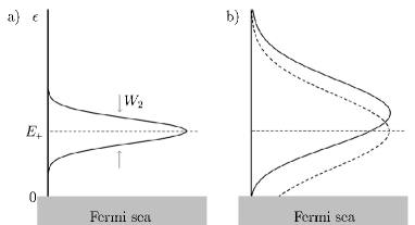
Figure 1: Width and position of the minimum for small (left) and large (right) perpendicular field as explained in the text.

After the substitution (10), the integration over $\omega$ in Eq. (5) can be performed exactly and we write the result as:

$$\delta\nu^{p}_{d}=\delta\nu_{d}^{m}+\delta\nu_{d}^{l}+\delta\nu_{d}^{f}\,,$$ (13)

where we separated different contributions based on their degree of divergence in the parallel field case: $\delta\nu_{d}^{m}$ gives the most divergent term (a $\delta$-function in $d=2$) which was considered in Ref. igor, , along with subleading terms; other subleading terms are collected in the the (less) divergent part $\delta\nu_{d}^{l}$; finally $\delta\nu_{d}^{f}$ contains only finite contributions and hence we do not need its explicit form. The relevant contributions are:

$$\frac{\delta\nu_{d}^{m}(\epsilon)}{\nu_{0}} = \frac{\Delta^{2}}{4\pi\nu_{0}\Omega}\,\mathrm{Im}\!\int\!\frac{d^{d}q}{(2\pi)^{d}}\,C^{2}(\epsilon-E_{+},\boldsymbol{q})$$

$$\times\left[\ln\frac{C(\epsilon-E_{Z},\boldsymbol{q})}{C(\epsilon-\Omega,\boldsymbol{q})}-\ln\frac{C(2\epsilon-E_{Z},\boldsymbol{q})}{C(-\Omega,\boldsymbol{q})}\right]$$

$$\frac{\delta\nu_{d}^{l}(\epsilon)}{\nu_{0}} = \frac{\Delta^{2}}{2\pi\nu_{0}\Omega}\,\mathrm{Im}\!\int\!\frac{d^{d}q}{(2\pi)^{d}}\,C(\epsilon-E_{+},\boldsymbol{q})$$

$$\quad\times\big{[}C(\epsilon-E_{Z},\boldsymbol{q})-C(2\epsilon-E_{Z},\boldsymbol{q})\big{]}$$

$$-\frac{i}{\epsilon-E_{-}}\big{[}C(2\epsilon-E_{Z},\boldsymbol{q})-C(-\Omega,\boldsymbol{q})\big{]}$$

with $E_{+}$ and $\Omega$ defined in Eqs. (1) and (2) respectively and we introduced:

$$E_{-}=\left(E_{Z}-\Omega\right)/2\,.$$ (15)

Note that Eq. (14) reduces to the perturbative result of Ref. igor, upon replacing the square bracket with $-2\pi i$. In what follows we retain only the most divergent terms, as finite and weakly divergent contributions have already been discarded in performing the replacement (10).

We now restrict our attention to the case $d=2$ with a non-zero perpendicular component of the magnetic field, so that we must use the substitution (11) and replace in Eqs. (14) the integrations over momentum with summations:

$$\int\!\frac{d^{2}q}{(2\pi)^{2}}\to\frac{\Omega_{H}}{4\pi D}\sum_{n=0}^{\infty}\,.$$ (16)

The result for the most divergent contribution is:

$$\begin{split}\frac{\delta\nu^{p}_{2}(\epsilon)}{\nu_{0}}=-\frac{W_{2}\pi^{2}}{\Omega_{H}}&\bigg{[}f\left(\frac{\epsilon-E_{+}}{\Omega_{H}};\frac{E_{-}}{\Omega_{H}}\right)\\ &+f\left(\frac{\epsilon-E_{+}}{\Omega_{H}};\frac{\epsilon-E_{-}}{\Omega_{H}}\right)\bigg{]}\,,\end{split}$$ (17)

where the energy

$$W_{2}\equiv\Delta^{2}/4g\Omega$$ (18)

characterizes the width of the tunneling anomaly in the parallel field and the function $f(a;b)$ is defined as:

$$f(a;b)=\mathrm{Im}\!\int^{\;b}_{-b}\frac{dt}{\pi^{3}t}\left[\psi^{\prime}\left(\frac{1}{2}-it-ia\right)-\psi^{\prime}\left(\frac{1}{2}-ia\right)\right]\!,$$ (19)

where $\psi^{\prime}$ is the derivative of the digamma function. The validity of Eq. (17) is restricted to the strong field regime:

$$\Omega_{H}\gg\pi^{2}W_{2}$$ (20)

in which the correction is indeed smaller than the bare DoS. As an example, we plot both Eq. (17) and the corresponding approximate formula of Ref. igor, in Fig. 2. We note that, in agreement with our previous discussion: the minimum is shifted to a higher energy; the contribution at small energies (near the Fermi sea) is suppressed; the overall shape is asymmetric about the minimum, in qualitative agreement with the experiments.ad1 ; ad2 In addition, the anomaly is smaller than the prediction of the approximate formula – this could be relevant in a quantitative comparison with experiments.

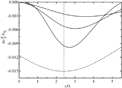
Figure 2: Tunneling anomaly in tilted field. The continuous lines are the correction $\delta\nu^{p}_{2}$ of Eq. (17) for $\theta=35^{\circ}$, $23^{\circ}$ and $16^{\circ}$ (top to bottom) with $g=5$, $E_{Z}=2.5\Delta$ and $g_{L}=2$. The vertical dotted line is at $\epsilon=E_{+}$. The dashed line is the approximate contribution of Ref. igor, for $\theta=35^{\circ}$, which can also be obtained by letting $b\to\infty$ in Eq. (19).

For the purpose of calculating the field-dependent position of the minimum, we can differentiate Eq. (17) and then expand the result to first order in $\delta=(\epsilon-E_{+})/\Omega_{H}$ by assuming $\delta\ll\frac{1}{2}$. Performing this calculation we find:

$$\frac{\delta\nu_{2}^{p\,\prime}}{\nu_{0}}=\frac{W_{2}\pi^{2}}{\Omega_{H}^{2}}\Big{[}\beta\delta+\gamma\Big{]}\,,$$ (21)

where

$$\beta=-\left[f^{\prime\prime}\!\!\left(0;\frac{E_{-}}{\Omega_{H}}\right)+f^{\prime\prime}\!\!\left(0;\frac{\Omega}{\Omega_{H}}\right)+\ddot{f}\left(0;\frac{\Omega}{\Omega_{H}}\right)\right]\lesssim 2\pi^{2}$$ (22)

with the prime denoting the derivative with respect to the first argument and the dot with respect to the second argument of $f$, and

$$\gamma=-\dot{f}\left(0;\frac{\Omega}{\Omega_{H}}\right)\geq\frac{2}{\pi^{3}}\psi^{\prime\prime}\!\left(\frac{1}{2}\right)\,.$$ (23)

While the above inequality is exact (and the equality is valid for $\Omega/\Omega_{H}=0$), the one in Eq. (22) should be understood as follows: for $E_{-},\Omega\gtrsim\Omega_{H}/3$ the approximate equality holds, while at lower values of these parameters is the upper limit that applies. Setting Eq. (21) to 0 and using for an estimate the limiting values of $\beta$ and $\gamma$, we find for the position $E^{*}$ of the minimum:

$$E^{*}=E_{+}+\alpha\Omega_{H}\,,\quad\alpha=-\frac{1}{\pi^{5}}\psi^{\prime\prime}\left(\frac{1}{2}\right)\simeq 0.055\,,$$ (24)

which generalizes the result of Ref. igor, and reduces to it for $\Omega_{H}=0$. The smallness of the constant $\alpha$ justifies a posteriori the expansion. In the experiment of Ref. ad2, , Eq. (24) has been successfully tested; below we comment on the applicability of this equation for experimentally relevant values of the parameters and we give more reliable estimates for the dependence of $E^{*}$ on $\Omega_{H}$.

According to the definitions (1), (2) and (15), the inequalities $E_{-}<\Omega\leq E_{+}\leq E_{Z}$ hold; in the experimentsad2 all these quantities are $\sim\Delta$. This means that $W_{2}\sim\Delta/4g\ll\Delta$ for good conductors. On the other hand

$$\frac{\Omega_{H}}{E_{Z}}=\frac{4}{g_{L}}g\sin\theta\,,$$ (25)

so that for “large” tilting angles we have $\Omega_{H}\gg E_{Z}$; thus we find that the condition (20) is experimentally satisfied. However the same reasoning shows that the conditions for the applicability of the upper limit estimate in Eq. (22) are easily violated. A more detailed study of the correction (17) shows that for the position $E^{*}$ of the minimum we can distinguish two regimes for different ranges of the parameter $\Omega_{H}/E_{Z}$, namely:

$$E^{*} = E_{+}+\alpha_{1}\left(\frac{\Omega_{H}}{E_{Z}},\frac{E_{Z}}{\Delta}\right)\Omega_{H}\ ,\quad 1\lesssim\frac{\Omega_{H}}{E_{Z}}\lesssim 7\qquad\$$ (26a)

$$E^{*} = 0.543E_{+}+\alpha_{\infty}\Omega_{H}\ ,\qquad\qquad\frac{\Omega_{H}}{E_{Z}}\gtrsim 7$$ (26b)

with

$$\alpha_{\infty}\simeq 0.144\,.$$ (27)

The coefficient $\alpha_{1}$ depends weakly on the field through $E_{Z}$; for fields larger than about twice the parallel critical field this dependence can be neglected and we find:

$$\alpha_{1}=\frac{3}{4}\frac{\Omega_{H}}{E_{Z}}\psi^{(2)}\left(\frac{1}{2}\right)/\psi^{(4)}\left(\frac{1}{2}\right)\simeq 0.016\frac{4}{g_{L}}g\sin\theta$$ (28)

independent of the field. The result (26a) is obtained by expanding $\beta$ [Eq. (22)] as a function of the quantities $E_{-}/\Omega_{H}$, $\Omega/\Omega_{H}$, while Eq. (26b) is found by taking the limit $g\to\infty$ in the derivative of Eq. (17): in this case the finite value of $\delta$ [defined before Eq. (21)] is calculated numerically and then we evaluate the coefficients of the first order corrections in $E_{-}/\Omega_{H},\,\Omega/\Omega_{H}$ – these are responsible for the suppression of the $E_{+}$ term. We stress that in the tilted field the linear dependence of the position of the minimum on the field is a robust prediction. We also notice that in the allowed region of the parameters, the coefficient $\alpha_{1}$ in front of $\Omega_{H}$ varies between $0.016$ and $0.112$, i.e. it agrees with $\alpha$ of Eq. (24) within a factor of 3; since it is also true that $\alpha_{\infty}/\alpha<3$, the estimate Eq. (24) is a correct order-of-magnitude one. Indeed that equation has been successfully applied in a study of a $g=5.6$ sample for which $\Omega_{H}/E_{Z}\lesssim 8$ in Ref. ad2, . Experiments in higher conductance samples, where $\Omega_{H}/E_{Z}\gg 7$, would enable to test Eq. (26b) directly: its simpler dependence on the physical parameters as compared to Eq. (26a) would make possible a more quantitative comparison between theory and experiments.

Up to now, we have not considered the phase relaxation effect of the (parallel component of the) magnetic field, since it can be usually neglected in the tilted field.igor This effect is accounted for by shifting the frequency in the definition (6) of the Cooperon: $\epsilon\to\epsilon+i/\tau_{H}$, withAA

$$1/\tau_{H}=\Omega_{H_{\parallel}}^{2}/48E_{T}\,.$$ (29)

Here $\Omega_{H_{\parallel}}$ is as in Eq. (12) but with $\cos\theta$ instead of $\sin\theta$ and the transverse Thouless energy is: $E_{T}=D/a^{2}$, where $a$ is the film’s width. In the parallel field, momentum integration in Eqs. (14) is straightforward; we do not give here the explicit answers (due to space limitations), but the qualitative results are the same as for the tilted field upon replacing $\Omega_{H}\to 1/\tau_{H}$. Also, we note that Eqs. (14) can be used to evaluate the correction to the DoS of superconducting wires; for both wires and the parallel field case, the one-loop approximation is valid when $W_{d}\tau_{H}\ll 1$.

In conclusion, we calculated the one-loop interaction correction to the Density of States for superconducting films in tilted field and in the paramagnetic phase. We found a minimum in the Density of States which shifts linearly with the applied field to higher energies, see e.g. Eq. (24); this dependence has been demonstrated experimentally.ad2

We thank I. Aleiner for the numerous interesting conversations; communications with P. Adams regarding the experimental results are gratefully acknowledged.

References

- (1) M. Tinkham, Introduction to superconductivity, (McGraw-Hill, New York, 1980); P. Fulde, Adv. Phys. 22, 667 (1973).
- (2) A.M. Clogston, Phys. Rev. Lett. 9, 266 (1962); B.S. Chandrasekhar, Appl. Phys. Lett. 1, 7 (1962).
- (3) H.Y. Kee, I.L. Aleiner and B.L. Altshuler, Phys. Rev. B 58, 5757 (1998).
- (4) B.L. Altshuler and A.G. Aronov, in Electron-Electron Interaction in Disordered Systems, edited by A.L. Efros and M. Pollak (North-Holland, Amsterdam, 1985).
- (5) W. Wu, J. Williams and P.W. Adams, Phys. Rev. Lett. 77, 1139 (1996); V. Yu. Butko, P. W. Adams, I.L. Aleiner, Phys. Rev. Lett. 82, 4284 (1999); P.W. Adams and V.Y. Butko, Physica B 284, 673 (2000).
- (6) X. S. Wu,P. W. Adams, G. Catelani, Phys. Rev. Lett. 95, 167001 (2005)
- (7) A.A. Abrikosov, L.P. Gorkov and I.E. Dzyaloshinski, Methods of Quantum Field Theory in Statistical Physics (Prentice-Hall, Englewood Cliffs, NJ, 1963).