Bright solitons in Bose-Fermi mixtures

Abstract

We consider the formation of bright solitons in a mixture of Bose and Fermi degenerate gases confined in a three-dimensional elongated harmonic trap. The Bose and Fermi atoms are assumed to effectively attract each other whereas bosonic atoms repel each other. Strong enough attraction between bosonic and fermionic components can change the character of the interaction within the bosonic cloud from repulsive to attractive making thus possible the generation of bright solitons in the mixture. On the other hand, such structures might be in danger due to the collapse phenomenon existing in attractive gases. We show, however, that under some conditions (defined by the strength of the Bose-Fermi components attraction) the structures which neither spread nor collapse can be generated. For elongated enough traps the formation of solitons is possible even at the “natural” value of the mutual Bose-Fermi (⁸⁷Rb -⁴⁰K in our case) scattering length.

Quantum degenerate atomic gases offer unique opportunities for investigating nonlinear properties of matter waves. Atomic Bose-Einstein condensation, first observed in $1995$ BEC , makes possible sources of sufficiently intense atomic matter waves allowing for the observation of nonlinear effects similar to those present in nonlinear optics. An important difference is that while the light must propagate through the nonlinear medium to produce the nonlinear effects, the nonlinearity is automatically present for atomic matter waves due to interactions between atoms. First confirmation of nonlinear atomic matter waves properties came in $1999$ when the four-wave-mixing phenomenon was observed in the Bose-Einstein condensate of sodium atoms 4WM . The second was a series of experiments discovering the solitonic behavior of atomic condensates. First, it was demonstrated with the help of the phase imprinting technique dark that the condensate wave function for repulsive interactions exhibits the dark solitonic solutions Zakharov . Next, also bright matter-wave solitons were created experimentally but this was achieved by other methods. In one of them, the interactions between atoms are changed from repulsive to attractive using the magnetically tuned Feshbach resonances technique bright , the other one lattice makes use of possibility of changing the sign of effective mass in the periodic potential (i.e., in the optical lattice), a concept developed in Ref. Lenz .

In Ref. TomekPRL we proposed a new way for generating bright solitons in repulsive Bose-Einstein condensates. The idea was to immerse the condensate in a degenerate gas of fermionic atoms which attract bosons. It turns out that for strong enough attraction between bosons and fermions the system starts to behave as a mixture of two effectively attractive gases even though none of the components alone is an attractive system. Therefore the formation of bright solitons becomes possible. These solitons are two-component peaks with much smaller number of fermions than bosons. However, in a three-dimensional space the atomic gases with attractive forces might show an instability due to the collapse. This is the main goal of this paper to answer the question whether solitons in a Bose-Fermi mixture can be generated despite of the existing instability driven by the attractive forces.

The system, we consider, is a Bose-Fermi mixture confined in a three-dimensional trap at zero temperature. We focus on the mixture of ⁸⁷Rb and ⁴⁰K atoms in their doubly spin polarized states. At zero temperature this system is described by the many-body wave function $\Psi({\bf x}_{1},...,{\bf x}_{N_{B}};{\bf y}_{1},...,{\bf y}_{N_{F}};t)$, where $N_{B}$ ($N_{F}$) is the number of bosons (fermions). To find the time evolution of the system we impose an assumption according to which the many-body wave function is given in terms of single-particle orbitals in the following way

$$\Psi({\bf x}_{1},...,{\bf x}_{N_{B}};{\bf y}_{1},...,{\bf y}_{N_{F}};t)=\prod_{i=1}^{N_{B}}\varphi^{(B)}({\bf x}_{i},t)$$

$$\times\frac{1}{\sqrt{N_{F}!}}\left|\begin{array}[]{lllll}\varphi_{1}^{(F)}({\bf y}_{1},t)&.&.&.&\varphi_{1}^{(F)}({\bf y}_{N_{F}},t)\\ \phantom{aaa}.&&&&\phantom{aaaaa}.\\ \phantom{aaa}.&&&&\phantom{aaaaa}.\\ \phantom{aaa}.&&&&\phantom{aaaaa}.\\ \varphi_{N_{F}}^{(F)}({\bf y}_{1},t)&.&.&.&\varphi_{N_{F}}^{(F)}({\bf y}_{N_{F}},t)\end{array}\right|$$ (6)

In fact, it is the simplest form that preserves the appropriate symmetry conditions for both the bosonic part and the spin-polarized fermionic subsystem.

To find the equations that govern the evolution of the single-particle wave functions we follow the formalism based on the Lagrangian density. Since the fermionic sample is spin-polarized the only interactions included are the contact boson-boson (assumed to be effectively repulsive) and boson-fermion (assumed to be attractive) ones. The time–dependent many–body Schrödinger equation is fully equivalent to the following Lagrangian density

$$\mathcal{L}=\frac{i\hbar}{2}\Psi^{*}\frac{\partial\Psi}{\partial t}-\frac{i\hbar}{2}\Psi\frac{\partial\Psi^{*}}{\partial t}-\frac{\hbar^{2}}{2m_{B}}\sum_{i=1}^{N_{B}}\nabla_{{\bf x}_{i}}\Psi^{*}\;\nabla_{{\bf x}_{i}}\Psi$$

$$-\frac{\hbar^{2}}{2m_{F}}\sum_{j=1}^{N_{F}}\nabla_{{\bf y}_{j}}\Psi^{*}\;\nabla_{{\bf y}_{j}}\Psi-\sum_{i=1}^{N_{B}}V_{trap}^{(B)}({\bf x}_{i})\;\Psi^{*}\Psi$$

$$-\sum_{j=1}^{N_{F}}V_{trap}^{(F)}({\bf y}_{j})\;\Psi^{*}\Psi-\sum_{i<i^{\prime}}V_{int}^{(BB)}({\bf x}_{i}-{\bf x}_{i^{\prime}})\;\Psi^{*}\Psi$$

$$-\sum_{i,j}V_{int}^{(BF)}({\bf x}_{i}-{\bf y}_{j})\;\Psi^{*}\Psi$$ (7)

treated as a function of the many-body wave function $\Psi({\bf x}_{1},...,{\bf x}_{N_{B}};{\bf y}_{1},...,{\bf y}_{N_{F}};t)$ and its time and spatial derivatives.

Therefore, the many-body wave function of the form (6) is inserted into the Lagrangian density (7). Next, we apply the mean-field approximation by integrating each term of (7) over all but one particular bosonic or fermionic coordinate (when the interaction term is considered both the one bosonic and one fermionic coordinates have to be left out). Utilizing the orthogonality properties of the fermionic orbitals (as well as neglecting $1$ in comparison with the number of bosons $N_{B}$) one gets the effective Lagrangian density

$$\mathcal{L^{\prime}}=\frac{i\hbar}{2}N_{B}\varphi^{(B)*}\frac{\partial\varphi^{(B)}}{\partial t}-\frac{i\hbar}{2}N_{B}\varphi^{(B)}\frac{\partial\varphi^{(B)*}}{\partial t}$$

$$+\frac{i\hbar}{2}\sum_{j=1}^{N_{F}}\varphi_{j}^{(F)*}\frac{\partial\varphi_{j}^{(F)}}{\partial t}-\frac{i\hbar}{2}\sum_{j=1}^{N_{F}}\varphi_{j}^{(F)}\frac{\partial\varphi_{j}^{(F)*}}{\partial t}$$

$$-\frac{\hbar^{2}}{2m_{B}}N_{B}\nabla\varphi^{(B)*}\nabla\varphi^{(B)}-\frac{\hbar^{2}}{2m_{F}}\sum_{j=1}^{N_{F}}\nabla\varphi_{j}^{(F)*}\nabla\varphi_{j}^{(F)}$$

$$-N_{B}V_{trap}^{(B)}|\varphi^{(B)}|^{2}-V_{trap}^{(F)}\sum_{j=1}^{N_{F}}|\varphi_{j}^{(F)}|^{2}$$

$$-\frac{1}{2}g_{B}N_{B}^{2}|\varphi^{(B)}|^{4}-g_{BF}N_{B}\sum_{j=1}^{N_{F}}|\varphi_{j}^{(F)}|^{2}\;|\varphi^{(B)}|^{2}$$ (8)

which depends on single-particle bosonic and fermionic orbitals and their spatial and time derivatives. Here, we already introduced the interaction strengths $g_{B}$ and $g_{BF}$ that determine relevant interatomic interactions and are related to the scattering lengths $a_{B}$ and $a_{BF}$ via formulas $4\pi\hbar^{2}a_{B}/m_{B}$ and $2\pi\hbar^{2}a_{BF}/\mu$, respectively ($m_{B}$ is a mass of ⁸⁷Rb atom and $\mu$ is a reduced mass of ⁸⁷Rb and ⁴⁰K atoms).

Having the effective single-particle Lagrangian density one can easily derive the corresponding Euler-Lagrange equations (here, $j=1,2,...,N_{F}$)

$$i\hbar\,\frac{\partial\varphi^{(B)}}{\partial t}=-\frac{\hbar^{2}}{2m_{B}}\nabla^{2}\varphi^{(B)}+V_{trap}^{(B)}\,\varphi^{(B)}$$

$$+\;g_{B}\,N_{B}\,|\varphi^{(B)}|^{2}\,\varphi^{(B)}+g_{BF}\sum_{j=1}^{N_{F}}|\varphi_{j}^{(F)}|^{2}\,\varphi^{(B)}$$

$$i\hbar\,\frac{\partial\varphi_{j}^{(F)}}{\partial t}=-\frac{\hbar^{2}}{2m_{F}}\nabla^{2}\varphi_{j}^{(F)}+V_{trap}^{(F)}\,\varphi_{j}^{(F)}$$

$$+\;g_{BF}\,N_{B}\,|\varphi^{(B)}|^{2}\,\varphi_{j}^{(F)}\;.$$ (9)

Neglecting the interaction between bosons and fermions results in a separation of the above equations; the first of them becomes then the Gross-Pitaevskii equation for a degenerate Bose gas whereas the rest describes the system of noninteracting fermions. However, when the Bose and Fermi components attract each other strongly enough the last term in the first equation can dominate over the term describing the bosonic mean-field energy causing effective attraction between bosons. We are going to investigate further this possibility.

We solve numerically the Eqs. (9) for a mixture of ⁸⁷Rb -⁴⁰K atoms confined in a three-dimensional elongated harmonic trap as well as in an atomic waveguide (obtained by releasing the axial confinement of the harmonic trap). We start from getting the ground state of a three-dimensional mixture in a harmonic trap. To this end, we pick up the atomic orbitals at zero time as they were the stationary solutions of Eqs. (9) assuming no interaction between bosons and fermions ($a_{BF}=0$). Therefore, the bosonic wave function is the solution of the Gross-Pitaevskii equation, whereas the fermionic orbitals are successive (with respect to the energy) eigenstates of the harmonic potential. Because of numerical limitations, the number of fermionic atoms is small (at most $15$ in our case) and since the trap is elongated only states with higher axial quantum number are populated (the radial quantum number equals zero). Next, we adiabatically increase the attraction between Bose and Fermi components.

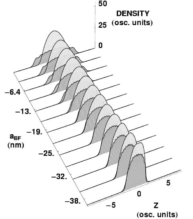
Figure 1: Axial density profiles of a three-dimensional Bose-Fermi mixture consisting of $100$ bosons (⁸⁷Rb atoms) and $10$ fermions (⁴⁰K atoms) confined in the harmonic trap with axial frequency $2\pi\times 1$ Hz and the radial one $2\pi\times 300$ Hz for bosonic component (corresponding trap frequencies for fermions are multiplied by a factor $1.473$). Interactions between bosons are determined by the “natural” scattering length $a_{B}=5.8$ nm whereas the strength of ⁸⁷Rb atoms -⁴⁰K atoms attraction is being changed. Dark (bright) shaded areas correspond to fermions (bosons). At zero attraction between fermions and bosons, fermions form a broad density distribution due to the Pauli exclusion principle. For strong enough attraction, however, fermions are pulled inside the bosonic cloud.

In Fig. 1 we plot the axial density (in units if $1/a_{ho}^{3}$, where $a_{ho}=(\hbar/m_{F}\omega_{z}^{(F)})^{1/2}$) of the ⁸⁷Rb -⁴⁰K mixture with $100$ bosons and $10$ fermions confined in the harmonic trap. The densities are normalized to one. The trap frequencies for bosons are $2\pi\times 1$ Hz ($2\pi\times 300$ Hz) in axial (radial) direction (corresponding frequencies for fermions are multiplied by a factor $1.473$). For weaker attraction between bosonic and fermionic atoms fermionic cloud broadens due to the Pauli exclusion principle. Stronger attraction, however, can overcome the repulsion caused by the Pauli exclusion principle and all fermions are pulled inside the bosonic cloud. Increasing further the attraction results in an extremely fast growth of the density at the center of the trap. In other words, the collapse of the mixture happens. It is shown in Fig. 2. This phenomenon was already observed experimentally collapse as well as extensively studied theoretically collthe . It is well known that such a behavior is attributed to the three-dimensional realm and does not happen in a one-dimensional geometry.

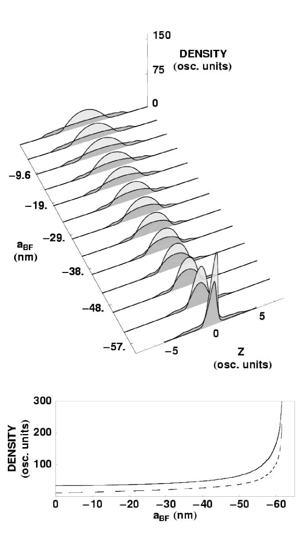
Figure 2: Illustration of a collapse phenomenon. All parameters but the number of fermions (that equals $15$ now) are the same as in Fig. 1. The lower panel shows the bosonic (solid line) and fermionic (dashed line) densities at the center of the trap as a function of the scattering length $a_{BF}$. The onset of the collapse at about $a_{BF}=-60$ nm is clearly visible.

Having the ground state of the ⁸⁷Rb -⁴⁰K mixture in the harmonic trap we can now reload the system to the atomic waveguide just by opening the trap in axial direction. Results of this procedure are presented in Figs. 3 and 5. The response of the system to the releasing of the axial confinement depends on the value of the scattering length $a_{BF}$. It turns out that for a particular trap geometry there is an interval of values of $a_{BF}$ with such a property that if $a_{BF}$ lies within this interval the two-component single-peak structure is formed which does not spread nor collapse. This case is shown in Fig. 3 where the axial confinement is linearly open in approximately $0.5$ s. The mixture looses $6$ bosons while both densities fit to each other and then apparently stays in the center of the trap without changing its shape. To check whether the mixture forms a soliton (or at least a solitary wave) we forced it to move by pushing along the waveguide direction the bosonic component. It is clear from Fig. 4 that bosons are able to pull fermions and both components stay together during the movement. Thus the mixture behaves as a solitary wave although some breathing of the structure is observed. The axial shapes of the densities resemble rather step-like function than the familiar solitonic secans-hyperbolicus shape. We find this shape as a typical (i.e., present in all geometries investigated) while changing the scattering length $a_{BF}$ by approaching the edge of the window supporting the existence of solitons, corresponding to the weaker attraction. For stronger attraction the shape is “more” solitonic (see Fig. 6). The soliton in Fig. 3 is $40$ $\mu$m long and the bosonic density is of the order of $10^{12}$ cm^-3.

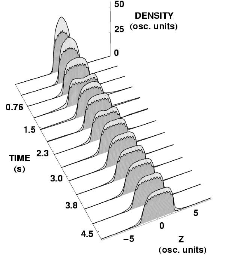
Figure 3: Two-component soliton standing at the center of the trap. The mutual scattering length equals $a_{BF}=-40$ nm. The axial confinement (the radial one is still kept on) is removed linearly within $0.5$ s. Bosonic and fermionic densities fit to each other in approximately $1$s (the system looses about $6$ bosons within this time) and later on the single peak two-component soliton is formed. Radial trap frequency is the same as that in the case of Fig. 1.

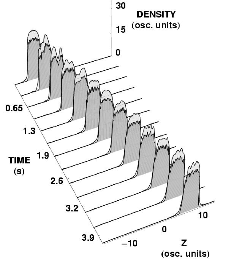
Figure 4: Illustration of the solitonic character of a structure obtained by releasing the axial confinement as in the case of Fig. 3. The structure is pushed along the axial direction (direction of no confinement) and is moving maintaining its shape (except small “breathing”). This is the case when the scattering length $a_{BF}$ lies within the window supporting the existence of bright solitons.

When the value of the scattering length $a_{BF}$ lies outside the window just discussed (i.e., the attraction between bosons and fermions is weak enough) we see the spreading of bosonic and fermionic clouds (Fig. 5). Here, $a_{BF}=-30$ nm and the attraction is too weak to glue the bosonic and fermionic clouds. Both clouds spread and eventually break into several smaller droplets. Fig. 5 shows that at least outermost droplets (consisting of $5$ fermions and $30$ bosons) demonstrate the solitonic behavior moving without changing their shapes. This observation supports the view that weaker attraction allows only for two-component solitons with small number of atoms (as opposed to what is reported in Ref. Adhikari ).

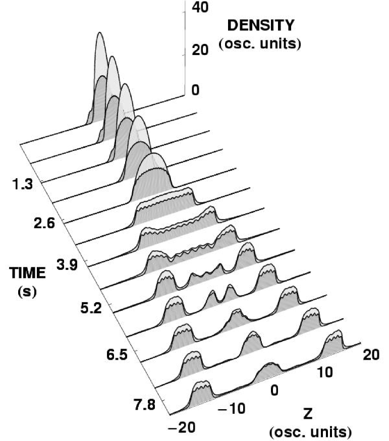
Figure 5: Nonsolitonic behavior of bosonic and fermionic clouds. The attraction between bosons and fermions is not strong enough ($a_{BF}=-30$ nm) and both densities are spreading. Later on, however, the clouds break into several pieces that move further without changing their shapes illustrating the rule that at weaker attraction solitons with smaller number of atoms are allowed. Here, the initial number of fermions equals $15$.

Finally, we consider the collision of two bright two-component solitons within the waveguide (Fig. 6). Both of them contains $6$ fermions and $100$ bosons. The right one stays at rest whereas the left one is forced to move by pushing the bosonic component. The left soliton is moving with the velocity $0.12$ mm/s. Moreover, the phase $\pi$ is added to the bosonic part of the soliton at rest, otherwise solitons merge when they meet at the center of the waveguide and collapse. This kind of behavior is similar to what happens for pure bosonic solitons governed by the Gross-Pitaevskii equation. In that case solitons repel or attract each other depending on the initial relative phase GPsol . If this relative phase equals $\pi$ the pure bosonic solitons always repel each other. This is what we observe in our numerical simulations, an example is given in Fig. 6. After collision the right soliton starts to move whereas the left one remains almost at rest. Usually, the transfer of some mass happens during the collision.

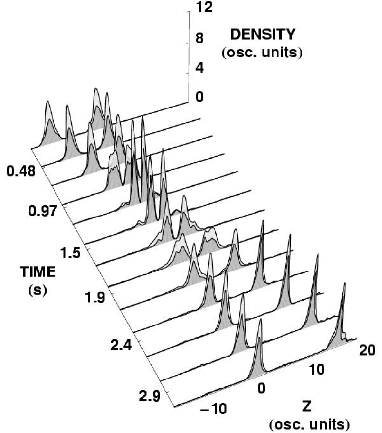
Figure 6: Collision of two solitons, each of them consisting of $6$ fermions and $100$ bosons. The left soliton is moving towards the right one being initially at rest. After collision (accompanied by the transfer of some atoms) the right soliton is moving and the left one is staying almost at rest. In this case $a_{BF}=-120$ nm and the trap parameters are $2\pi\times 1$ Hz in the axial direction and the $2\pi\times 30$ Hz for the radial one for bosonic component.

To summarize our numerical work we present in Table 1 some numbers characterizing the formation of single-peak two-component bright solitons. In particular, two last columns give approximate values of the critical mutual scattering lengths $a_{BF}^{cr}$ (the mixture spreads for the weaker attraction than $a_{BF}^{cr}$) and the values of $a_{BF}^{col}$ determining the onset of the collapse for various radial confinements. Thus, there exist windows supporting the existence of stable structures that maintain their shapes while moving and may survive the collisions (although some atoms are usually transfered during the collision). Such structures can be called solitons. The critical value of the scattering length can be also estimated as in the Ref. TomekPRL . Based on the first equation of a set of Eqs. (9) the condition for the system to enter the phase when the bosonic component becomes the gas of effectively attractive atoms (and hence allowing for the generation of bright solitons) is written as $g_{B}n_{B}=|g_{BF}^{cr}|n_{F}$, where $n_{B}=N_{B}|\varphi^{(B)}|^{2}$ and $n_{F}=\sum_{i}^{N_{F}}|\varphi_{i}^{(F)}|^{2}$ are the bosonic and fermionic densities at the center. This criterion gives the values: $-86$ nm, $-40$ nm, and $-14$ nm for the radial confinements: $2\pi\times 30$ Hz, $2\pi\times 300$ Hz, and $2\pi\times 1000$ Hz, respectively, what remains in a good agreement with the values obtained directly from the numerical simulations.

Table 1: Parameters characterizing the formation of single-peak two-component bright solitons.

$\nu^{(B)}_{r}$[Hz]	$N_{B}$	$N_{F}$	$a_{BF}^{cr}$[nm]	$a_{BF}^{col}$[nm]
30	100	6	-90	-135
300	94	10	-35	-62
1000	64	15	-17	-44

In Table 1 we put also the numbers of fermionic and bosonic atoms within the single-peak solitons. They are obtained in the following way. For each geometry (i.e., the radial confinement) we start from the three-dimensional harmonic trap ground state consisting of $100$ bosons and $10$ or $15$ fermions. After releasing the axial confinement the excess of atoms (bosons or fermions) flows out of the system. For example, for the radial frequency $\nu_{r}^{(B)}=30$ Hz the mixture looses $4$ fermions and then behaves as a soliton (to get more fermions within the peaks the initial number of bosons would have to be bigger). For stronger radial confinement the mixture expels the excessive bosons. We have checked that for $\nu_{r}^{(B)}=2000$ Hz there exists a soliton at the natural value of the scattering length $a_{BF}$ (equal to $-13.2$ nm, Jin ). Our simulations show that at small values of $|a_{BF}|$ only solitons with small numbers of atoms exist, the excessive bosons or fermions just leak out of the system. Our preliminary results based on the three-dimensional variational analysis within the hydrodynamic model of a Bose-Fermi mixture tobe also demonstrate that solitons with large numbers of atoms require stronger attraction between fermionic and bosonic components.

In conclusion, we have shown that bright solitons can be generated in a Bose-Fermi mixture trapped in a three-dimensional elongated harmonic potential. For that the attraction between bosonic and fermionic atoms has to be strong enough changing in this way the repulsive interactions among bosons to the attractive ones. Simultaneously, the attractive forces induced in the bosonic cloud has to be weak enough to avoid the collapse. It turns out that there exist windows in the values of the rubidium-potassium scattering length within which the single-peak two-component structures neither spreading nor collapsing (therefore called by us solitons) can be formed. Those windows are shifting towards the region of less negative Bose-Fermi scattering length (weaker attraction) while elongating the trap making thus possible the formation of solitons even at the natural strength of the boson-fermion attraction.

- (1) M.H. Anderson, J.R. Ensher, M.R. Matthews, C.E. Wieman, and E.A. Cornell, Science 269, 198 (1995); K.B. Davis, M.-O. Mewes, M.R. Andrews, N.J. van Druten, D.S. Durfee, D.M. Kurn, and W. Ketterle, Phys. Rev. Lett. 75, 3969 (1995); C.C. Bradley, C.A. Sackett, J.J. Tollett, and R.G. Hulet, Phys. Rev. Lett. 75, 1687 (1995) and Erratum 79, 1170(E) (1997).
- (2) L. Deng, E.W. Hagley, J. Wen, M. Trippenbach, Y. Band, P.S. Julienne, J.E. Simsarian, K. Helmerson, S.L. Rolston, and W.D. Phillips, Nature 398, 218 (1999).
- (3) S. Burger, K. Bongs, S. Dettmer, W. Ertmer, K. Sengstock, A. Sanpera, G.V. Shlyapnikov, and M. Lewenstein, Phys. Rev. Lett. 83, 5198 (1999); J. Denschlag, J.E. Simsarian, D.L. Feder, C.W. Clark, L.A. Collins, J. Cubizolles, L. Deng, E.W. Hagley, K. Helmerson, W.P. Reinhardt, S.L. Rolston, B.I. Schneider, W.D. Phillips, Science 287, 97 (2000); B.P. Anderson, P.C. Haljan, C.A. Regal, D.L. Feder, L.A. Collins, C.W. Clark, and E.A. Cornell, Phys. Rev. Lett. 86, 2926 (2001).
- (4) V.E. Zakharov and A.B. Shabat, Zh. Eksp. Teor. Fiz. 61, 118 (1971) [Sov. Phys. JETP 34, 62 (1972)]; 64, 1627 (1973) [Sov. Phys. JETP 37, 823 (1973)].
- (5) L. Khaykovich, F. Schreck, G. Ferrari, T. Bourdel, J. Cubizolles, L.D. Carr, Y. Castin, and C. Salomon, Science 296, 1290 (2002); K.E. Strecker, G.B. Partridge, A.G. Truscott, and R.G. Hulet, Nature 417, 150 (2002).
- (6) B. Eiermann, Th. Anker, M. Albiez, M. Taglieber, P. Treutlein, K.-P. Marzlin, and M.K. Oberthaler, Phys. Rev. Lett. 92, 230401 (2004).
- (7) G. Lenz, P. Meystre, and E.M. Wright, Phys. Rev. A 50, 1681 (1994).
- (8) T. Karpiuk, M. Brewczyk, S. Ospelkaus-Schwarzer, K. Bongs, M. Gajda, and K. Rza̧żewski, Phys. Rev. Lett. 93, 100401 (2004).
- (9) G. Modugno, G. Roati, F. Riboli, F. Ferlaino, R.J. Brecha, and M. Inguscio, Science 297, 2240 (2002); C. Ospelkaus, S. Ospelkaus, K. Sengstock, and K. Bongs, cond-mat/ 0507219 (2005).
- (10) R. Roth and H. Feldmeier, Phys. Rev. A 65, 021603(R) (2002); R. Roth, Phys. Rev. A 66, 013614 (2002); S. K. Adhikari, Phys. Rev. A 70, 043617 (2004); T. Karpiuk, M. Brewczyk, M. Gajda, and K. Rza̧żewski, J. Phys. B 38, L215 (2005).
- (11) S. K. Adhikari, Phys. Rev. A 72, 053608 (2005).
- (12) L.D. Carr and J. Brand, Phys. Rev. A 70, 033607 (2004); J.P. Gordon and H.A. Haus, Opt. Lett. 11, 665 (1986); P.V. Elyutin, A.V. Buryak, V.V. Gubernov, R.A. Sammut, and I.N. Towers, Phys. Rev. E 64, 016607 (2002).
- (13) J. Goldwin, S. Inouye, M.L. Olsen, B. Newman, B.D. DePaola, and D.S. Jin, Phys. Rev. A 70, 021601(R) (2004). Recently, another value of the scattering length ( nm) has been measured, F. Ferlaino, C. D’Errico, G. Roati, M. Zaccanti, M. Inguscio, and G. Modugno, cond-mat/ 0510630 (2005).
- (14) to be published