Kondo effect in triple quantum dots

Abstract

Numerical analysis of the simplest odd-numbered system of coupled quantum dots reveals an interplay between magnetic ordering, charge fluctuations and the tendency of itinerant electrons in the leads to screen magnetic moments. The transition from local-moment to molecular-orbital behavior is visible in the evolution of correlation functions as the inter-dot coupling is increased. Resulting novel Kondo phases are presented in a phase diagram which can be sampled by measuring the zero-bias conductance. We discuss the origin of the even-odd effects by comparing with the double quantum dot.

One of the main notions in molecular physics is the formation of extended molecular orbitals when atoms are brought together to bind into a molecule. Using atomic manipulation capabilities of modern low-temperature scanning tunneling microscopes, the delocalization of electrons can now be directly studied by adding individual atoms to a molecule-like chain of atoms on a flat substrate wallis2002 . Alternatively, one can study the transition from localized to extended behavior in the systems of coupled quantum dots, which can also be considered as a variety of artificial molecules. Unlike in atomic chains, bonding in coupled dots can be continuously adjusted using the pinch gate electrodes hatano2004 .

The Kondo effect is a many-body phenomenon due to interaction between a localized spin and free electrons. It leads to an increased conductance through nanostructures and it was first observed in single quantum dots (QD) goldhaber98 . The conductance as a function of temperature, gate and bias voltages is in agreement with theoretical predictions that such dots behave rather universally as single magnetic impurities pustilnik04 and can be modelled using single impurity Anderson and Kondo models. By analogy, the Kondo effect in multiple-dot systems can be described using multiple-impurity Anderson model.

Measurements of the transport properties of multiple QD systems indicate that the conductance is significantly different for even and odd number of dots waugh95 . Double QD (DQD) systems are the simplest representation of the two-impurity Anderson model. Their phase diagram features single-impurity Kondo effect, two-electron Kondo effect and a suppressed-conductance state due to anti-ferromagnetic (AFM) coupling between the dots georges99 ; kikoin01 . Good understanding of these different regimes was obtained using various numerical techniques izumida00 ; lopez02 ; cornaglia05 ; bulka04 .

Much less is known about odd-number systems of coupled QD. Even the properties of the triple quantum dot (TQD), the simplest member of the family, have not been systematically resolved to date. There is clearly a regime of Coulomb blockade at intermediate temperatures stafford94 ; chen94 . Some properties of the Kondo regime at low temperatures are known from previous studies using the perturbation theory oguri01 , the numerical renormalization group hewson05 , scaling techniques kuzmenko02 , the slave-boson mean-field theory jiang05 and embedding busser04 . Some of these methods lead to conflicting results for the same type of TQD, so further studies using reliable numerical techniques are required.

In this Letter, we study the TQD using two complementary numerical methods: the constrained path Monte Carlo method (CPMC) zhang and the Gunnarsson-Schönhammer variational method (GS) gunnarsson85 . The conductance is calculated using the sine method rejec03 . We analyze the low-temperature phases of the TQD embedded in series between two metallic leads, Fig. 1.

Figure 1: (Color online) The triple quantum dot embedded between two leads

The TQD is modelled as a cluster of three equal QD described by Hamiltonians $H_{i}=\sum_{\sigma}\epsilon_{d}n_{i\sigma}+Un_{i\uparrow}n_{i\downarrow}$, $i=1,2,3$, where the on-site energy $\epsilon_{d}$ can be varied using the gate voltage and $U$ is the electron-electron (e-e) repulsion. The dots are interconnected with hopping matrix element $t^{\prime\prime}$ and are symmetrically coupled to the leads with hopping matrix element $t^{\prime}$. We choose the chemical potential in the middle of the band, so that the model is particle-hole (p-h) symmetric for $\epsilon_{d}+U/2=0$.

For large $t^{\prime\prime}/U$, the system is in the molecular-orbital Kondo regime when occupancy $\langle n\rangle=\sum_{i\sigma}\langle n_{i\sigma}\rangle$ is odd. In the $U\to 0$ limit, the conductance through the TQD as a function of the gate voltage exhibits three peaks corresponding to resonant tunneling through distinct noninteracting levels: non-bonding, bonding and anti-bonding molecular-orbitals with energies $\epsilon_{\pm,0}=\pm\sqrt{2}t^{\prime\prime},0$ and hybridizations $\Gamma_{\pm,0}=\frac{3}{8}\Gamma,\frac{1}{2}\Gamma$, where $\Gamma=2t^{\prime 2}/t$. When interactions are switched on, the middle peak remains at $\epsilon_{d}+U/2=0$, while the side-peaks are symmetrically shifted to $\epsilon_{d}+U/2\sim\pm(\sqrt{2}t^{\prime\prime}+\frac{5}{16}U)+{\cal O}(U^{2}/t^{\prime\prime})$ in the molecular limit $\Gamma\to 0$. The $U$-term is a consequence of the inter-orbital repulsion. The intra-orbital e-e repulsion is then given by $U_{\pm}\sim\frac{3}{8}U+{\cal O}(U^{2}/t^{\prime\prime})$ and $U_{0}\sim\frac{1}{2}U+{\cal O}[U^{3}/(t^{\prime\prime})^{2}]$. The Kondo temperatures $T_{\pm,0}$ for levels $(\pm,0)$ can be determined from the Haldane formula haldane for the single QD using the corresponding parameters $U_{\pm,0}$.

The zero-temperature phase diagram of TQD exhibits several phases with enhanced conductance, Fig. 2. In the molecular-orbital Kondo regime (shaded regions labelled ’M1’ and ’M3’) the conductance is $G/G_{0}\gtrsim 0.5$ for low temperatures $T\ll T_{\pm,0}$, while for intermediate temperatures $T_{\pm,0}\ll T\ll\Gamma$ the system is in the Coulomb blockade regime with $G\sim 0$ except along the border lines. Lightly shaded stripes of width $\sim\Gamma/2$ represent the transition regions, where $G/G_{0}\lesssim 0.5$. Phase ’M2’ is a non-conductive even-occupancy spin-zero phase, where two electrons occupy the same molecular-orbital.

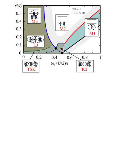
Figure 2: (Color online) M1, M3: molecular-orbital Kondo regime with $\langle n\rangle\sim 1,3$. M2: non-conductive even-occupancy state. L3: local Kondo regime with $\langle n\rangle\sim 3$. TSK: two-stage Kondo regime. K2: local double Kondo regime with $\langle n\rangle\sim 2$.

In Fig. 3 we present the zero-bias conductance $G$ along with the total occupancy $\langle n\rangle$ as a function of the gate voltage for a range of $t^{\prime\prime}$ and for fixed $U/t=1$ and $\Gamma/t=0.18$, calculated with various methods as discussed below. For $t^{\prime\prime}/U\geq 0.2$, the system is in the molecular-orbital regime. As the occupancy monotonically decreases from 6 (full TQD) to 0 (empty TQD), the conductance exhibits well resolved peaks when occupancy is odd and valleys when occupancy is even goldhaber98 .

As the TQD coupled to the leads is Fermi liquid hewson05 , the zero temperature linear conductance is given by the sine formula derived in Ref. rejec03, , $G=G_{0}\sin^{2}\left[\frac{N}{4t}(E_{0}-E_{\pi})\right]$. Here $G_{0}=2e^{2}/h$ and $E_{0,\pi}$ are the ground state energies of a large $N$-site auxiliary ring with embedded interacting system, with periodic and anti-periodic boundary conditions, respectively. Ground state properties are determined using CPMC and GS methods.

In the CPMC method zhang , the ground state wave function $|\Psi_{0}\rangle$ is projected from a known trial function $|\Psi_{T}\rangle$ using a branching random walk that generates an over-complete space of Slater determinants $|\phi\rangle$ and can be written as $|\Psi_{0}\rangle=\sum_{\phi}c_{\phi}|\phi\rangle$, where $c_{\phi}>0$. To completely specify $|\Psi_{0}\rangle$, only determinants satisfying $\langle\Psi_{T}|\phi\rangle>0$ are needed, because $|\Psi_{0}\rangle$ resides in either of two degenerate halves of the Slater determinant space separated by a nodal plane. In this manner, the minus-sign problem is alleviated. Extensive testing has demonstrated a significant insensitivity of the results to reasonable choices of $|\Psi_{T}\rangle$ zhang ; Bonca . The CPMC calculations were performed on a ring of 100-180 sites. As the number of sites with interaction is small, CPMC produces ground state energies with excellent precision, typically of the order of $\Delta E/E=10^{-6}$.

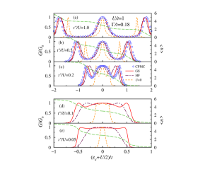
Figure 3: (Color online) $G/G_{0}$ and $\langle n\rangle$ vs. $\epsilon_{d}+U/2$ (proportional to the gate voltage) for various inter-dot hopping $t^{\prime\prime}$. Note enhanced energy scale in panels (d) and (e). Error bars of CPMC are smaller than the size of circles. For comparison, we also show the Hartree-Fock (HF) as well as $U=0$ results.

In the GS method, the ground state energies are determined as the minimum energy of the variational wave function $|\Psi\rangle=\sum_{\lambda=1}^{64}c_{\lambda}P_{\lambda}\left|\tilde{0}\right\rangle$, where $P_{\lambda}$ are the projection operators for the three sites of the molecule, e.g., $P_{1}=\prod_{i,\sigma}(1-n_{i,\sigma})$, $P_{2}=n_{1,\uparrow}(1-n_{1,\downarrow})\prod_{i=2,3,\sigma}(1-n_{i,\sigma})$, …, $P_{64}=\prod_{i,\sigma}n_{i,\sigma}$. The vacuum state $\left|\tilde{0}\right\rangle$ corresponds to the Fermi sea of a non-interacting Hamiltonian $\tilde{H}$ with renormalized parameters. The variational wave function is exact in the $U\to 0$ and $t^{\prime}\to 0$ limits and the test results for a single Anderson site perfectly match the exact Bethe Ansatz results rejec03 ; comment ; mravlje05 .

For $t^{\prime\prime}/U\geq 0.2$ the conductance obtained with CPMC and GS methods shows good agreement. For lower $t^{\prime\prime}/U$ the CPMC method is no more applicable since due to the computational restriction on the system size its energy resolution is insufficient to describe the small Kondo scale finitesize .

The local regime emerges when $t^{\prime\prime}/U$ decreases below $\sim 0.2$. The orbital description breaks down as the orbitals start to overlap which leads to qualitative changes in the system properties. The relevant interaction becomes $U$ rather than $U_{\pm,0}$. As presented in Fig. 3(d,e), $G/G_{0}\sim 1$ near the symmetric point $\epsilon_{d}+U/2=0$, while in the charge transfer region, $|\epsilon_{d}+U/2|\sim U/2$, the conductance exhibits humps separated by dips. Due to larger $U$, the Kondo scale in the local regime decreases. Note that for $t^{\prime\prime}/U\lesssim 0.2$ the HF calculation starts to deviate, signaling the onset of the strong coupling regime. For even lower $t^{\prime\prime}/U$ the HF curves differ qualitatively from correct results.

The relation between the DQD and the TQD in the local regime is first considered for $\langle n\rangle\sim 2$. This corresponds to the p-h symmetric point of the DQD, where the two relevant energy scales are known georges99 to be the exchange energy $J=4(t^{\prime\prime})^{2}/U$ and the Kondo temperature $T_{1K}=T_{K}(U,\Gamma_{1})$, with $\Gamma_{1}=\Gamma/2$, which is the hybridization of a single impurity coupled to one lead haldane . In TQD, two electrons can reduce their energy by hopping within the TQD, therefore instead of $J$ the relevant scale is the kinetic energy linear in $t^{\prime\prime}$. The transition between the phase ’M2’ to the phase ’K2’ (see Fig. 2) occurs when $\sqrt{2}t^{\prime\prime}\sim 2T_{1K}$. The phase ’K2’ is a double Kondo phase, where the spin of each electron is screened by electrons from the nearest lead.

The behavior of the TQD near the p-h symmetric point, $\langle n\rangle\sim 3$, is different from the behavior of the DQD near its p-h symmetric point, $\langle n\rangle\sim 2$, due to the different properties of integer and half-integer spin states. It is also different from the behavior of the DQD near its charge-transfer points, $\langle n\rangle\sim 1,3$, which exhibit Kondo effect only for large $t^{\prime\prime}/U$. The TQD is fully conducting at the p-h symmetric point for any $t^{\prime\prime}$ and as $t^{\prime\prime}/U$ is reduced the system goes continuously through three different Kondo regimes. The molecular-orbital ‘M3’ regime has already been discussed. For low $t^{\prime\prime}/U$ there are two different regimes of local Kondo physics. (i) In the local Kondo ’L3’ regime for $J>2T_{1K}$, the TQD is antiferromagnetically rigid and electrons form an ordered chain with spin $1/2$ that exhibits the usual Kondo effect. Transition between molecular-orbital ’M3’ and local ’L3’ is quite soft and determined by the competition between kinetic ($t^{\prime\prime}$) and magnetic ($J$) scale. (ii) In the two-stage Kondo ’TSK’ regime for $J<2T_{1K}$, each side QD ($i=1,3$) couples with $\Gamma_{1}$ to the nearest lead and their spin is screened at $T\lesssim T_{1K}$, while due to very weak coupling the remaining spin is screened at much lower temperature $T_{2K}\propto T_{1K}\exp(-cT_{1K}/J)$ with $c\sim 1$ cornaglia05 .

In Table 1 we give quantitative relations for lines between different phases of the system. Boundaries between phases M1, M2, M3, and L3 are determined in the molecular $\Gamma\to 0$ limit to the lowest non-trivial order in $U$ (or $t^{\prime\prime}$). The expressions are in excellent agreement with numerical results. We note that all transitions are smooth (cross-overs) and there are no abrupt phase transitions.

Phase 1	Phase 2	Condition
empty	M1	$\delta\sim U/2+\sqrt{2}t^{\prime\prime}$
M1	M2	$\begin{cases}\delta\sim U/2+3(t^{\prime\prime})^{2}/U,&t^{\prime\prime}\lesssim U\\ \delta\sim U/8+\sqrt{2}t^{\prime\prime},&\ t^{\prime\prime}\gtrsim U\end{cases}$
M2	M3, L3	$\begin{cases}\delta\sim U/2-\sqrt{2}t^{\prime\prime}+3(t^{\prime\prime})^{2}/U,&t^{\prime\prime}\lesssim U\\ \delta\sim U\left(1/4+\tfrac{3}{512}(U/t^{\prime\prime})^{2}\right),&t^{\prime\prime}\gtrsim U\end{cases}$
M3	L3	$\sqrt{2}t^{\prime\prime}\sim J$
M2	K2	$\sqrt{2}t^{\prime\prime}+3(t^{\prime\prime})^{2}/U\sim 2\min(T_{1K},\Gamma_{1})$
L3	TSK	$J\sim 2T_{1K}$

Table 1: Definitions of boundaries and cross-over regions between various phases in Fig. 2. Here $\delta=\epsilon_{d}+U/2$ and $J=4(t^{\prime\prime})^{2}/U$.

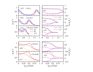
Figure 4: (Color online) Moments $\langle S_{z}^{2}\rangle$ vs. $\epsilon_{d}+U/2$, left panels (a1)-(e1). Spin-spin correlation functions $\langle S_{iz}S_{jz}\rangle$ for $(ij)=(11)$, $(22)$, $(12)$, and $(13)$ as calculated from the GS wave function, right panels (a2)-(e2).

The finger-print of the Kondo physics are not only the broadened conductance peaks, but also the formation of a local moment in the TQD, which is then screened by the electrons in the leads. In Fig. 4 we present $\langle S_{z}^{2}\rangle$, where $S_{z}=\sum_{i=1}^{3}S_{iz}$ is the z-component of the total spin of the TQD (left panels), and local $i=j$, nearest neighbor $(ij)=(12)$ and next-nearest neighbor $(ij)=(13)$ spin-spin correlations $\langle S_{iz}S_{jz}\rangle$ (right panels). For large $t^{\prime\prime}$, formation of local moment (spin-doublet) is evident, but the spin is not saturated, $4\langle S_{z}^{2}\rangle<1$. For $t^{\prime\prime}\to 0$ and $\langle n\rangle\sim 2$, increased $4\langle S_{z}^{2}\rangle>1$ illustrates formation of the ’K2’ phase with large local moment and the absence of inter-site spin correlations. The two electrons are relatively independent and therefore total spin is enhanced (note that for two uncorrelated spins $4\langle S_{z}^{2}\rangle=2$). Each electron is coupled by the Kondo mechanism to the adjacent lead. For $\langle n\rangle\sim 3$, we see that neighboring spins tend to anti-align while left-most and right-most spins align as $t^{\prime\prime}/U$ is reduced, which represents formation of an antiferromagnetically ordered chain when we enter the ’L3’ phase.

Charge fluctuations $\Delta n^{2}=\langle(n-\langle n\rangle)^{2}\rangle$ and the corresponding charge susceptibility $\chi_{c}=-(\pi\Gamma/4)\partial\langle n\rangle/\partial\epsilon_{d}$ exhibit double peaks at positions of the conductance peaks as an additional characteristic of the Kondo effect mravlje05 and start to build a dip in the symmetric point for $t^{\prime\prime}/U<0.2$ (not shown here). This additionally signals the transition from orbital to local Kondo regime and is in agreement with local spin formation shown in Fig. 4(d,e).

In summary, we have determined the phase diagram of the TQD. For strong inter-dot coupling, the system behaves as an artificial molecule. The extended ”molecular orbitals” are filled consecutively and the system exhibits the usual Kondo effect when the number of confined electrons is odd. For weak inter-dot coupling, local spin behavior is observed. The cross-over from extended to local Kondo physics is illustrated by the smooth evolution of the spin-spin correlation functions. In the vicinity of the p-h symmetric point, the TQD tends to an antiferromagnetically ordered state when the inter-dot coupling is decreased. For extremely weak coupling, the Kondo screening of local moments occurs in two stages. In the charge transfer regime the left and right sites tend to form two relatively independent Kondo correlated states.

We expect that in the limit of extremely weak coupling, other complex phases might exist in the immediate vicinity of the $\epsilon_{d}=0$ point, where occupancy of the central dot changes abruptly. Furthermore, we believe that the properties of all $n$ dot systems (with $n$ odd) are similar at the p-h symmetric point: as the inter-dot coupling is decreased, the molecular-orbital Kondo regime $Mn$ is followed by an antiferromagnetically locked Kondo regime $Ln$ and then by a two-stage Kondo regime.

We thank Y. Avishai, Y. Meir, and A. C. Hewson for helpful discussions. Authors acknowledge support from the Ministry of Higher education, Science and Technology of Slovenia under grant Pl-0044 and from Ben-Gurion University.

References

- (1) T. M. Wallis and N. Nilius and W. Ho, Phys. Rev. Lett. 89, 236802 (2002).
- (2) T. Hatano et al., Phys. Rev. Lett. 93, 066806 (2004).
- (3) D. Goldhaber-Gordon et al., Nature (London) 391, 156 (1998); S. M. Cronenwett et al., Science 281, 540 (1998).
- (4) M. Pustilnik and L. Glazman, J. Phys. Condens. Matter 13, R513 (2004).
- (5) F. R. Waugh et al., Phys. Rev. Lett. 75, 705 (1995); N. J. Craig et al., Science 304, 565 (2004).
- (6) A. Georges and Y. Meir, Phys. Rev. Lett. 82, 3508 (1999).
- (7) K. Kikoin and Y. Avishai, Phys. Rev. Lett. 86, 2090 (2001).
- (8) W. Izumida and O. Sakai, Phys. Rev. B 62, 10260 (2000).
- (9) R. López, R. Aguado, and G. Platero, Phys. Rev. Lett. 89, 136802 (2002).
- (10) P. S. Cornaglia and D. R. Grempel, Phys. Rev. B 71, 075305 (2005).
- (11) B. R. Bulka and T. Kostyrko, Phys Rev. B 70, 205333 (2004).
- (12) C. A. Stafford and S. Das Sarma, Phys. Rev. Lett. 72, 3590 (1994).
- (13) G. Chen, G. Klimeck, S. Datta, G. Chen, and W. A. Goddard III, Phys. Rev. B 50, 8035 (1994).
- (14) A. Oguri, Phys. Rev. B 63, 115305 (2001);
- (15) A. Oguri and A. C. Hewson, J. Phys. Soc. Jpn. 74, 988 (2005); A. Oguri, Y. Nisikawa, and A. C. Hewson, ibid., 2554 (2005).
- (16) T. Kuzmenko, K. Kikoin, and Y. Avishai, Phys. Rev. Lett. 89, 156602 (2002); Europhys. Lett. 64, 218 (2003); T. Kuzmenko, Ph.D. Thesis, Ben-Gurion University (2005).
- (17) Zhao-tan Jiang, Qing-feng Sun, and Yupeng Wang, Phys. Rev. B 72, 045332 (2005).
- (18) C. A. Büsser, A. Moreo, and E. Dagotto, Phys. Rev. B 70, 035402 (2004.)
- (19) S. Zhang, J. Carlson and J. E. Gubernatis, Phys. Rev. Lett., 74, 3652 (1995); Phys. Rev. B 55, 7464 (1997); J. Carlson, J. E. Gubernatis, G. Ortiz, and Shiwei Zhang, Phys. Rev. B 59, 12788 (1999); M. Guerrero, G. Ortiz, and J. E. Gubernatis, Phys. Rev. B 59, 1706 (1999);Phys. Rev. B 62, 600 (2000).
- (20) O. Gunnarsson and K. Sch ̈onhammer, Phys. Rev. B 31, 4815 (1985).
- (21) T. Rejec and A. Ramšak, Phys. Rev. B 68, 035342 (2003); ibid. 033306 (2003); R. Molina et al., Phys. Rev. B 67, 235306 (2003).
- (22) ; F. D. M. Haldane, Phys. Rev. Lett. 40, 416 (1978).
- (23) J. Bonča and J. E. Gubernatis, Phys. Rev. B 58, 6992 (1998).
- (24) J. Bonča, A. Ramšak, and T. Rejec, cond-mat/0407590.
- (25) J. Mravlje, A. Ramšak, and T. Rejec, Phys. Rev. B 72, 121403(R) (2005).
- (26) In CPMC up to 180 sites were used to model the leads, while in GS we used 2000 sites which yields fully converged results.