Critical Exponents from General Distributions of Zeroes

Abstract

All of the thermodynamic information on a statistical mechanical system is encoded in the locus and density of its partition function zeroes. Recently, a new technique was developed which enables the extraction of the latter using finite-size data of the type typically garnered from a computational approach. Here that method is extended to deal with more general cases. Other critical points of a type which appear in many models are also studied.

and

1 Introduction

Phase transitions are of central interest in statistical physics and related fields. Second-order transitions are signaled by divergences and characterised by critical exponents (e.g., $\alpha$ for the specific heat and $\nu$ for the correlation length in the temperature driven case). Such non-analytic behaviour is only present in systems of infinite extent and is therefore inaccessible to Monte Carlo simulations, which are restricted to a finite number of degrees of freedom.

Traditionally, however, finite-size scaling (FSS) may be used to extract thermodynamic information from such systems. FSS, based on the hypothesis that there are only two relevant length scales (namely the correlation length of the infinite system and its finite-size counterpart), typically only allows determination of ratios of critical exponents associated with thermodynamic functions, such as $\alpha/\nu$. An exception is the correlation length critical exponent $\nu$ which can be directly extracted from logarithmic derivatives of magnetization moments or from the slope of the Binder parameter $\sim\langle m^{2k}\rangle/\langle m^{k}\rangle^{2}$, $k=1,2,\dots$. Alternatively one may also consider the scaling behaviour of pseudocritical points. The latter, defined as the extrema of thermodynamic functions, approach the transition point as $L^{-\lambda}$, where $L$ denotes the linear extent of the system and $\lambda$ is the so-called shift exponent. The exponent $\lambda$ coincides with $1/\nu$ in many models, but this is not a consequence of FSS and is not always true. See, e.g., [1] for a review of the recent literature concerning this point. A further complication that arises from the latter approach is that such a fit involves three parameters and is non-linear, so usually is quite unstable and often inaccurate.

An increasingly popular approach is the use of FSS of the zeroes of the partition function. FSS of the lowest zeroes in the complex temperature plane (Fisher zeroes) provides a direct and accurate method to extract the exponent $\nu$, and the imaginary parts of the lowest zeroes (labelled by an index $j$) scale with lattice extent as ${\rm{Im}}z_{j}\sim L^{-1/\nu}$. The real part of the lowest partition function zero is another pseudocritical point, generally scaling as $L^{-\lambda}$.

It has long been known that a full understanding of the properties of the bulk system requires knowledge of the density of zeroes too. Until recently, determination of the density from finite-size Monte Carlo data was considered difficult if not impossible. The source of the difficulties is that it involves reconstruction of a continuous density function from a discrete data set as the density of zeroes for a finite system essentially consists of a set of delta functions.

Recent considerations have bypassed these difficulties by focusing instead on the integrated density of zeroes [2]. In particular, this new approach facilitates measurement of the strength of the transition through direct determination of $\alpha$ (as opposed to traditional FSS measurements of the ratio $\alpha/\nu$). While the new technique proved successful, it was limited to systems where the zeroes fall on curves in the complex parameter plane and where the zeroes are non-degenerate. While these two properties are common to most models in statistical physics, they are not generic and a host of examples now exist where the zeroes are distributed across a two-dimensional region and/or occur in degenerate sets. Here, the new technique is extended to deal with such general distributions of zeroes [3].

2 General Distributions of Zeroes

When the partition function, $Z_{V}$, for a system of volume $V=L^{d}$ ($d$ being the dimensionality of the system) can be written as a polynomial in an appropriate function, $z$, of temperature, field or of a coupling parameter, one has $Z_{V}(z)\propto\prod_{j}{(z-z_{j}(V))}$ where $j$ labels the zeroes. In the general case where the distribution of zeroes is two-dimensional, the free energy may be expressed as $f_{V}=\int\!\!\int g_{V}(x,y)\ln{(z-z_{c}-x-iy)}dxdy$, where $g_{V}$ is the density of zeroes and $(x,y)$ give their location in the complex plane with the critical point, $z_{c}$, as the origin. In the infinite-volume case, Stephenson has shown that the density near a second-order transition point satisfies a certain homogeneous partial differential equation, the solution of which may be written as $g_{\infty}(x,y)=y^{1-\alpha-m}f(x/y^{m})$, where $m$ is related to the shape of the locus [4]. Integrating out the $x-$direction, and integrating up to a point $r$ in the $y-$direction gives the cumulative density there to be

$$G_{\infty}(r)\propto r^{2-\alpha}\,.$$ (1)

From this expression, the exponent $\alpha$ may be directly measured provided that a sensible definition for the cumulative density of zeroes can be applied to a finite system. Such a function is defined as follows. If the $j^{\rm{th}}$ zero is $n$-fold degenerate the densities to its immediate left and right are given by $VG_{V}(r)=j-1$ and $j+n-1$ respectively. The density at the $j^{\rm{th}}$ zero, $r_{j}$, is then defined as an average:

$$G_{L}(r_{j})=\frac{1}{V}\left(j+\frac{n}{2}-1\right)\,.$$ (2)

Combined with (1), this allows direct determination of the critical exponent $\alpha$.

3 Applications

We apply the new technique to Ising models in two dimensions for which the zeroes are calculable and which possess each of the new features we wish to encapsulate. In each case, the real, physical, critical point is characterized by $\alpha=0$.

Brascamp-Kunz lattice with anisotropic couplings: The finite-size, standard, nearest-neighbour, square lattice Ising model has been solved in two dimensions for certain sets of boundary conditions including those first studied by Brascamp and Kunz [5]. There, periodic boundary conditions are used in one direction, while at the extremities in the other direction the spins are fixed to $+$ on the one hand and the alternating sequence $+-+-\dots$ on the other.

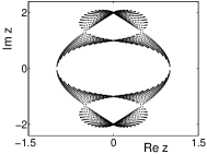
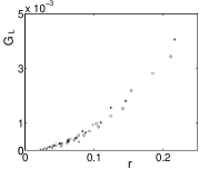
Figure 1: The zeroes (top) for the anisotropic $L=40$ Brascamp-Kunz Ising model with $J^{\prime}/J=3$ and their density distribution (bottom) near $z=1$ for $L=40$–$140$ and $j=1$ ($\times$), $j=2$ ($+$), $j=3$ ($*$), $j=4$ ($\circ$), $j=5$ ($\Box$), $j=6$ ($\diamond$), $j=7$ ($\bullet$) and $j=8$ ($\star$).

For a lattice of linear extent $L$ with anisotropic couplings $J$ and $J^{\prime}$, the partition function then takes the form of a single product (as opposed to a sum of four such products, which is the case when periodic boundary conditions in both directions are used [6]), greatly ameliorating the computation of its zeroes [1]. The zeroes are easily determined numerically and are distributed across a two-dimensional region in the $z=2\sinh(2\beta)$ plane as shown in Fig. 1 for $J^{\prime}/J=3$ (with $\beta=J/k_{B}T$). The zeroes impact onto the real axis at the point $z=1$ and the critical behaviour is dominated by the zeroes close by. The cumulative density distribution for this set of zeroes is also plotted in Fig. 1. That the curve goes through the origin indicates the presence of a transition and an appropriate fit yields $\alpha=-0.016(32)$ compatible with expectations.

Bathroom-tile lattice: Two-dimensional distribution of zeroes may also be obtained from systems with isotropic couplings as demonstrated in [7] where the system is described in detail. In principle the full finite-size partition function is a sum of four product terms. One may construct Brascamp-Kunz type boundary conditions for this lattice, which would have the effect of projecting out one of these terms in the expression for the partition function. Alternatively, and more conveniently, one may discretize one of the terms in the partition function with periodic boundary conditions and assume for the purposes of the analysis herein that the scaling behaviour of that term is generic. Indeed, since we are essentially interested in testing the scaling of the cumulative density of zeroes rather than formulating the finite lattice models themselves, this is sufficient for our purposes (see also [3]).

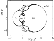
Figure 2: The zeroes (top) for the $L=40$ bathroom-tile Ising model and their density (bottom) near the ferromagnetic critical point from data with $L=40$–$200$ and $j=1$-$4$ ($\times$), $j=5$-$12$ ($+$), $j=13$-$16$ ($*$), $j=17$-$24$ ($\circ$), $j=25$-$32$ ($\Box$), $j=33$-$40$ ($\diamond$) and $j=41$-$44$ ($\bullet$).

The zeroes of such a term have varying degrees of degeneracy and are depicted in the complex $z^{\prime}=\exp{(-2\beta)}$ plane in Fig. 2, where AFM, PM, FM and O₁ indicate the anti-ferromagnetic, paramagnetic, ferromagnetic and unphysical phases, respectively. The physical ferromagnetic critical point is given by $z^{\prime}=0.249\,038\,4\dots$ and the cumulative density of zeroes nearby is also depicted in the figure. A fit yields $\alpha=0.002(18)$, consistent with zero. There is also an antiferromagnetic transition point at $z^{\prime}=4.015\,445\,4\dots$. A density fit to the zeroes nearby yields $\alpha=0.0006(163)$, again compatible with $\alpha=0$.

Since the finite-size partition function is known exactly in this case, and is a convenient single product, it is possible to analytically extract the $\nu$ and $\lambda$ exponents from conventional FSS of the lowest lying zeroes. Indeed, one finds that $\nu=1$ (which again gives $\alpha=0$ through hyperscaling) and $\lambda=2$ in both the ferromagnetic and antiferromagnetic cases.

Complex vertices:

It has been pointed out that unphysical singular points (i.e., points for which there is no real $\beta$) may be considered as ordinary critical points with distinctive critical exponents (see, e.g., [7] and references therein).

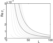
Figure 3: Finite-size dependency of the zeroes close to the complex singular point $z=i$ in the isotropic Brascamp-Kunz model. The dotted lines scale as ${\rm{Re}}z_{j}\sim L^{-3}$ and the solid lines as ${\rm{Re}}z_{j}\sim L^{-2}$.

For the example of the two-dimensional Ising model with Brascamp-Kunz boundary conditions, the complex vertex points at $z=i$ and $2i$ in Fig. 1 are thus also of interest. However, analysis shows these not to be of the conventional type. Fig. 3 is a plot showing how the first few zeroes in the simpler isotropic model approach such a vertex at $z=i$ with increasing lattice size.

To understand the unusual behaviour depicted, an analytic approach is required. A full scaling analysis of this model at its real transition point $z=1$ is given in [1]. For a square lattice of linear extent $L$, the zeroes, which are labelled $z_{ij}$, are given by

$${\rm{Re}}z_{ij} = \frac{1}{2}\left(\cos{\theta_{i}}+\cos{\phi_{j}}\right)\,,$$

$${\rm{Im}}z_{ij} = \sqrt{1-({\rm{Re}}z_{ij})^{2}}\,,$$ (3)

where $\theta_{i}=(2i-1)\pi/L$ and $\phi_{j}=j\pi/(L+1)$. Expanding the cosines for large $L$ gives ${\rm{Re}}z_{ij}=1+{{\mathcal{O}}}(L^{-2})$ and ${\rm{Im}}z_{ij}={\mathcal{O}}(L^{-1})$, recovering $\lambda=2$ and $\nu=1$, as above. For ${\rm{Re}}z_{ij}$ close to $1$ (the physical critical point), both $i$ and $j$ have to be close to zero and the above expansion is legitimate. However, close to the unphysical point $z=i$, the two cosines in (3) have to cancel and the expansion is no longer valid. Cancellations of this type remove the leading $L^{-2}$ term for the approach to the vertex of the first few zeroes (which then scale as $L^{-3}$) and do not occur at a real critical point. This explains the odd scaling behaviour in Fig. 3 and demonstrates the dangers inherent to a restricted traditional analysis of leading zeroes. This and related issues will be elaborated upon elsewhere.

The situation close to the unphysical points $z^{\prime}=-0.601\,231\,8\dots$ and $z^{\prime}=-1.663\,251\,9\dots$ in Fig. 2 is more conventional and density analyses yield $\alpha=0.007(12)$ and $\alpha=-0.0095(123)$ respectively. The exponents $\nu$ and $\lambda$ may also be extracted analytically here and one again finds $\nu=1$, $\lambda=2$. It is interesting to note that these are yet more cases where $\nu$ does not coincide with $\lambda$ [1].

References

- [1] W. Janke, R. Kenna, Finite-size scaling and corrections in the Ising model with Brascamp-Kunz boundary conditions, Phys. Rev. B 65 (6) (2002) 064110.
- [2] W. Janke, R. Kenna, The strength of first and second order phase transitions from partition function zeroes, J. Stat. Phys. 102 (5/6) (2001) 1211–1227.
- [3] W. Janke, D. Johnston, R. Kenna, Phase transition strength through densities of general distributions of zeroes, Nucl. Phys. B 682 (FS) (2004) 618–634.
- [4] J. Stephenson, On the density of partition function temperature zeros, J. Phys. A 20 (13) (1987) 4513–4519.
- [5] H. Brascamp, H. Kunz, Zeroes of the partition function for the Ising model in the complex temperature plane, J. Math. Phys. 15 (1) (1974) 65–66.
- [6] B. Kaufman, Crystal statistics II. partition function evaluated by spinor analysis, Phys. Rev. 76 (8) (1949) 1244–1252.
- [7] V. Matveev, R. Shrock, Complex-temperature properties of the Ising model on 2D heteropolygonal lattices, J. Phys. A 28 (18) (1995) 5235–5256.