Topological Objects in Two-gap Superconductor:I

Abstract

We discuss topological objects, in particular the non-Abrikosov vortex and the magnetic knot made of the twisted non-Abrikosov vortex, in two-gap superconductor. We show that there are two types of non-Abrikosov vortex in Ginzburg-Landau theory of two-gap superconductor, the D-type which has no concentration of the condensate at the core and the N-type which has a non-trivial profile of the condensate at the core, under a wide class of realistic interaction potential. Furthermore, we show that we can construct a stable magnetic knot by twisting the non-Abrikosov vortex and connecting two periodic ends together, whose knot topology $\pi_{3}(S^{2})$ is described by the Chern-Simon index of the electromagnetic potential. We discuss how these topological objects can be constructed in $\rm MgB_{2}$ or in liquid metallic hydrogen.

I Introduction

Topological objects, in particular finite energy topological objects (monopoles, vortices, skyrmions, and knots), have played increasingly important role in physics dirac ; abri ; skyr ; fadd1 ; prl01 . In condensed matter the best known topological objects are the Abrikosov vortex in one-gap superconductors and similar ones in Bose-Einstein condensates and superfluids, which have been the subject of intensive studies. A recent advent of two-component Bose-Einstein condensates and two-gap superconductors bec ; sc , however, has opened up an exciting new possibility for us to construct far more interesting topological objects in laboratories. It has already been shown that non-Abrikosov vortices whose topology is fixed by $\pi_{2}(S^{2})$ and finite energy topological knots whose topology is fixed by $\pi_{3}(S^{2})$ exist in these condensed matters ijpap ; ruo ; pra05 ; prb05 ; baba1 ; cm2 . The reason for this is that these condensed matters are made of two components which can be viewed as an $SU(2)$ multiplet. In general this type of topological objects is possible when one has a multi-component condensates, which allows the non-Abelian topology.

The purpose of this paper is to discuss new topological objects in Ginzburg-Landau theory of two-gap superconductor in detail. With a most general $U(1)\times U(1)$ symmetric potential which can describe a wide class of two-gap superconductors we first show that there are two types of non-Abrikosov vortex, D-type and N-type, in two-gap superconductor. The D-type has no concentration of the condensate at the core, but the N-type has a non-trivial profile of the condensate at the core. The reason why the two-gap superconductor has two types of vortex is that the vortex in two-gap superconductor allows two different boundary conditions. In terms of topology the non-Abrikosov vortex is described by two types of topology, non-Abelian $\pi_{2}(S^{2})$ topology or Abelian $\pi_{1}(S^{1})$ topology. And within the same topology both D-type and N-type vortices exist. In particular, there are infinitely many D-type vortices classified by the natural number $k$ which have the same topology. Moreover, the magnetic flux of these non-Abrikosov vortices can be integral or fractional, and the integral flux vortex has the $\pi_{2}(S^{2})$ topology and the fractional flux vortex has the $\pi_{1}(S^{1})$ topology. We show that the N-type vortex has a $2\pi n/g$-flux or a fractional flux (a fraction of $2\pi n/g$), but the D-type vortex has $2\pi k/g$ more flux than the N-type vortex. These characteristic features of the non-Abrikosov vortex are clearly absent in the Abrikosov vortex which carries $2\pi n/g$-flux whose topology is fixed by $\pi_{1}(S^{1})$.

Next, we show that the non-Abrikosov vortex can be twisted to form a helical vortex which is periodic in $z$-axis. More importantly, we show that we can construct a stable magnetic knot in two-gap superconductors by smoothly bending the helical vortex and connecting the periodic ends together. The vortex ring acquires the knot topology $\pi_{3}(S^{2})$ which is fixed by the Chern-Simon index of the electromagnetic potential. Because of the helical structure of the magnetic flux the knot has two magnetic flux linked together, one around the knot tube and one along the knot, whose linking number is given by the knot quantum number. And the flux trapped inside the vortex ring provides a stabilizing repulsive force which prevents the collapse of the knot, because it can not be squeezed out. This means that the knot has dynamical (as well as topological) stability.

It is well-known that multi-gap superconductor may have interband Josephson interaction maz . We consider a most general quartic Josephson interaction in two-gap superconductor, and show that the presence of the Josephson interaction does not affect the existence of the above topological objects, but can alter the shape of the solutions drastically. We show that in the presence of the Josephson interaction we have a magnetic vortex which can be viewed as a bound state of two fluxes, which becomes a braided magnetic vortex when twisted.

The paper is organized as follows. In Section II we discuss a most general quartic potential in Ginzburg-Landau theory of two-gap superconductor in mean field approximation, and study the vacuum structure. In Section III we show that the Ginzburg-Landau theory of two-gap superconductor can be understood as a theory of $CP^{1}$ field coupled to a scalar field and the electromagnetic field, and argue that the topology of the theory can be described by the $CP^{1}$ field and the electromagnetic field. In Section IV we construct the non-Abrikosov vortex in two-gap superconductor, and show that there are two types of boundary condition which allow two types of magnetic vortex, the D-type which has no concentration of condensate at the core and the N-type which has a non-trivial concentration of condensate at the core. Moreover we show that there are two types of topology, non-Abelian $\pi_{2}(S^{2})$ and Abelian $\pi_{1}(S^{1})$, which describes these vortices. We show that the magnetic flux of these vortices can be integral or fractional depending on the parameters of the potential, but the D-type vortex has $2\pi k/g$ more flux than the N-type vortex. In Section V we show that we can construct a helical magnetic vortex in two-gap superconductor, by twisting the non-Abrikosov vortex and making it periodic in $z$-axis. In Section VI we construct the magnetic knot bending the helical vortex and connecting the periodic ends together, and show that the knot topology $\pi_{3}(S^{2})$ is described by the Chern-Simon index of the electromagnetic potential. In Section VII we consider the Josephson interaction, and show that the inclusion of the Josephson interaction does not affect the existence of the topological objects in two-gap superconductor but alter the shape of the solutions drastically. In Section VIII we discuss the non-Abelian superconductivity which can describe a two-gap superconductor made of two condensates which carry opposite charge, and argue that the non-Abelian superconductivity can be realized in liquid metallic hydrogen (LMH). Finally in Section IX we discuss the physical implications of our results, and discuss how one can identify these topological objects in $\rm MgB_{2}$ and LMH.

II Effective potential of Two-gap Superconductor

In mean field approximation the free energy of the two-gap superconductor could be expressed by baba1 ; maz ; baba2

$${\cal H}=\displaystyle\frac{\hbar^{2}}{2m_{1}}|(\mbox{\boldmath$\nabla$}+ig\mbox{\boldmath$A$})\tilde{\phi}_{1}|^{2}+\displaystyle\frac{\hbar^{2}}{2m_{2}}|(\mbox{\boldmath$\nabla$}+ig\mbox{\boldmath$A$})\tilde{\phi}_{2}|^{2}$$

$$+\tilde{V}(\tilde{\phi}_{1},\tilde{\phi}_{2})+\displaystyle\frac{1}{2}(\mbox{\boldmath$\nabla$}\times\mbox{\boldmath$A$})^{2},$$ (1)

where $\tilde{V}$ is the effective potential. We choose the potential to be the most general quartic potential which has the $U(1)\times U(1)$ symmetry,

$$\tilde{V}=\displaystyle\frac{\tilde{\lambda}_{11}}{2}|\tilde{\phi}_{1}|^{4}+\tilde{\lambda}_{12}|\tilde{\phi}_{1}|^{2}|\tilde{\phi}_{2}|^{2}+\displaystyle\frac{\tilde{\lambda}_{22}}{2}|\tilde{\phi}_{2}|^{4}$$

$$-\tilde{\mu}_{1}|\tilde{\phi}_{1}|^{2}-\tilde{\mu}_{2}|\tilde{\phi}_{2}|^{2},$$ (2)

where $\tilde{\lambda}_{ij}$ are the quartic coupling constants and $\tilde{\mu}_{i}$ are the chemical potentials of $\tilde{\phi}_{i}~{}(i=1,2)$. One might like to include the Josephson interaction to the potential which breaks the $U(1)\times U(1)$ symmetry down to $U(1)$. The Josephson interaction will be discussed separately in the following. But as we will see, the inclusion of the Josephson interaction does not alter the qualitative features of the topological objects we discuss in this paper.

With the normalization of $\tilde{\phi}_{1}$ and $\tilde{\phi}_{2}$ to $\phi_{1}$ and $\phi_{2}$,

$$\phi_{1}=\displaystyle\frac{\hbar}{\sqrt{2m_{1}}}\tilde{\phi}_{1},\;\;\;\;\phi_{2}=\frac{\hbar}{\sqrt{2m_{2}}}\tilde{\phi}_{2}.$$ (3)

one can simplify the above Hamiltonian (1) to

$${\cal H}=|(\mbox{\boldmath$\nabla$}+ig\mbox{\boldmath$A$})\phi|^{2}+V(\phi_{1},\phi_{2})$$

$$+\displaystyle\frac{1}{2}(\mbox{\boldmath$\nabla$}\times\mbox{\boldmath$A$})^{2},$$ (4)

where $V$ is the normalized potential,

$$V=\displaystyle\frac{\lambda_{11}}{2}|\phi_{1}|^{4}+\lambda_{12}|\phi_{1}|^{2}|\phi_{2}|^{2}+\displaystyle\frac{\lambda_{22}}{2}|\phi_{2}|^{4}$$

$$-\mu_{1}|\phi_{1}|^{2}-\mu_{2}|\phi_{2}|^{2}$$

$$=\displaystyle\frac{\lambda_{11}}{2}\big{(}|\phi_{1}|^{2}-\hat{\phi}_{1}^{2}\big{)}^{2}+\displaystyle\frac{\lambda_{22}}{2}\big{(}|\phi_{2}|^{2}-\hat{\phi}_{2}^{2}\big{)}^{2}$$

$$+\lambda_{12}\big{(}|\phi_{1}|^{2}-\hat{\phi}_{1}^{2}\big{)}\big{(}|\phi_{2}|^{2}-\hat{\phi}_{2}^{2}\big{)}+V_{0},$$

$$\hat{\phi}_{1}^{2}=\displaystyle\frac{\mu_{1}\lambda_{22}-\mu_{2}\lambda_{12}}{\Delta},~{}~{}~{}~{}~{}\hat{\phi}_{2}^{2}=\displaystyle\frac{\mu_{2}\lambda_{11}-\mu_{1}\lambda_{12}}{\Delta}$$

$$V_{0}=-\displaystyle\frac{\lambda_{11}\mu_{2}^{2}+\lambda_{22}\mu_{1}^{2}-2\lambda_{12}\mu_{1}\mu_{2}}{2\Delta},$$

$$\Delta=\lambda_{11}\lambda_{22}-\lambda_{12}^{2}.$$ (5)

Notice that the potential can also be written as

$$V=\displaystyle\frac{1}{2\lambda_{11}}\Big{[}(\lambda_{11}|\phi_{1}|^{2}+\lambda_{12}|\phi_{2}|^{2}-\mu_{1})^{2}$$

$$+\Delta\big{(}|\phi_{2}|^{2}-\hat{\phi}_{2}^{2}\big{)}^{2}\Big{]}+V_{0}$$

$$=\displaystyle\frac{1}{2\lambda_{22}}\Big{[}(\lambda_{12}|\phi_{1}|^{2}+\lambda_{22}|\phi_{2}|^{2}-\mu_{2})^{2}$$

$$+\Delta\big{(}|\phi_{1}|^{2}-\hat{\phi}_{1}^{2}\big{)}^{2}\Big{]}+V_{0}.$$ (6)

From now on we will assume that all coupling constants except $\lambda_{12}$ are positive.

To find the vacuum of the potential let

$$\displaystyle\frac{\partial V}{\partial|\phi_{1}|^{2}}=\lambda_{11}|\phi_{1}|^{2}+\lambda_{12}|\phi_{2}|^{2}-\mu_{1}=0,$$

$$\displaystyle\frac{\partial V}{\partial|\phi_{2}|^{2}}=\lambda_{12}|\phi_{1}|^{2}+\lambda_{22}|\phi_{2}|^{2}-\mu_{2}=0,$$ (7)

and find the extremum

$$|\phi_{1}|^{2}=\hat{\phi}_{1}^{2},~{}~{}~{}~{}~{}|\phi_{2}|^{2}=\hat{\phi}_{2}^{2}.$$ (8)

To check whether this extremum is the maximum or minimum, consider the Hessian

$$\det H=\det\displaystyle\frac{\partial^{2}V}{\partial|\phi_{i}|^{2}\partial|\phi_{j}|^{2}}=\lambda_{11}\lambda_{22}-\lambda_{12}^{2}$$

$$=\Delta.$$ (9)

There are three possibilities; positive, zero, or negative $\Delta$. We consider each case separately.

A. $\Delta>0$: In this case we have $\lambda_{12}^{2}<\lambda_{11}\lambda_{22}$, and the extremum (8) becomes the local minimum. But since $|\phi_{i}|$ have to be positive we have the following vacuum

$$\Bigg{(}\matrix{<|\phi_{1}|>\cr<|\phi_{2}|>}\Bigg{)}=\Bigg{(}\matrix{\hat{\phi}_{1}\cr\hat{\phi}_{2}}\Bigg{)},$$ (10)

for $\lambda_{12}\leq 0$ or for

$$0<\lambda_{12},~{}~{}~{}\displaystyle\frac{\lambda_{12}}{\lambda_{22}}<\displaystyle\frac{\mu_{1}}{\mu_{2}}<\displaystyle\frac{\lambda_{11}}{\lambda_{12}}.$$ (11)

Notice that both $<|\phi_{1}|>$ and $<|\phi_{2}|>$ are non-vanishing. But for

$$0<\lambda_{12},~{}~{}~{}\displaystyle\frac{\lambda_{12}}{\lambda_{22}}<\displaystyle\frac{\lambda_{11}}{\lambda_{12}}<\displaystyle\frac{\mu_{1}}{\mu_{2}},$$ (12)

we have the following vacuum from (6),

$$\Bigg{(}\matrix{<|\phi_{1}|>\cr<|\phi_{2}|>}\Bigg{)}=\Bigg{(}\matrix{\sqrt{\mu_{1}/\lambda_{11}}\cr 0}\Bigg{)},$$ (13)

Finally, when

$$0<\lambda_{12},~{}~{}~{}\displaystyle\frac{\mu_{1}}{\mu_{2}}<\displaystyle\frac{\lambda_{12}}{\lambda_{22}}<\displaystyle\frac{\lambda_{11}}{\lambda_{12}},$$ (14)

we can always transform this case to the case (12) by re-labeling $\phi_{1}$ and $\phi_{2}$ as $\phi_{2}$ and $\phi_{1}$, so that in this case we can assume that the vacuum is still given by (13) without loss of generality.

B. $\Delta=0$: In this case we have $\lambda_{12}^{2}=\lambda_{11}\lambda_{22}$, and the potential (5) is reduced to

$$V=\displaystyle\frac{1}{2\lambda_{11}}\Big{[}\big{(}\lambda_{11}|\phi_{1}|^{2}+\lambda_{12}|\phi_{2}|^{2}-\mu_{1}\big{)}^{2}$$

$$-2(\mu_{2}\lambda_{11}-\mu_{1}\lambda_{12})|\phi_{2}|^{2}\Big{]}$$

$$=\displaystyle\frac{1}{2\lambda_{22}}\Big{[}\big{(}\lambda_{12}|\phi_{1}|^{2}+\lambda_{22}|\phi_{2}|^{2}-\mu_{2}\big{)}^{2}$$

$$-2(\mu_{1}\lambda_{22}-\mu_{2}\lambda_{12})|\phi_{1}|^{2}\Big{]}.$$ (15)

So for $\lambda_{12}<0$, the potential becomes unbounded from below, so that it has no minimum. For

$$0<\lambda_{12},~{}~{}~{}~{}~{}\displaystyle\frac{\lambda_{11}}{\lambda_{12}}=\displaystyle\frac{\lambda_{12}}{\lambda_{22}}<\displaystyle\frac{\mu_{1}}{\mu_{2}},$$ (16)

we have the following vacuum

$$\Bigg{(}\matrix{<|\phi_{1}|>\cr<|\phi_{2}|>}\Bigg{)}=\Bigg{(}\matrix{\sqrt{\mu_{1}/\lambda_{11}}\cr 0}\Bigg{)}.$$ (17)

Next, consider the case

$$0<\lambda_{12},~{}~{}~{}~{}~{}\displaystyle\frac{\mu_{1}}{\mu_{2}}<\displaystyle\frac{\lambda_{11}}{\lambda_{12}}=\displaystyle\frac{\lambda_{12}}{\lambda_{22}}.$$ (18)

But this can be transformed to (16) with the re-labeling. So we can assume that the vacuum is given by (17) without loss of generality. Finally, when

$$\displaystyle\frac{\mu_{1}}{\mu_{2}}=\displaystyle\frac{\lambda_{11}}{\lambda_{12}}=\displaystyle\frac{\lambda_{12}}{\lambda_{22}},$$ (19)

we have the degenerate vacuum

$$\mu_{1}<|\phi_{1}|>^{2}+\mu_{2}<|\phi_{2}|>^{2}=\displaystyle\frac{\mu_{1}\mu_{2}}{\lambda_{12}}.$$ (20)

This case includes the special (and familiar) $SU(2)$ symmetric case

$$\lambda_{11}=\lambda_{12}=\lambda_{22}=\lambda,~{}~{}~{}u_{1}=\mu_{2}=\mu,$$

$$<|\phi_{1}|>^{2}+<|\phi_{2}|>^{2}=\displaystyle\frac{\mu}{\lambda}.$$ (21)

In this case the Hamiltonian (4) has the full $SU(2)$ symmetry.

C. $\Delta<0$: In this case we have $\lambda_{12}^{2}>\lambda_{11}\lambda_{22}$, and the extremum (8) becomes the local maximum. So the minimum state must satisfy

$$|\phi_{1}|^{2}|\phi_{2}|^{2}=0.$$ (22)

Now, by inspection one can show that when

$$0<\lambda_{12},~{}~{}~{}\displaystyle\frac{\lambda_{11}}{\lambda_{12}}<\sqrt{\displaystyle\frac{\lambda_{11}}{\lambda_{22}}}<\displaystyle\frac{\mu_{1}}{\mu_{2}},$$ (23)

the vacuum must be

$$\Bigg{(}\matrix{<|\phi_{1}|>\cr<|\phi_{2}|>}\Bigg{)}=\Bigg{(}\matrix{\sqrt{\mu_{1}/\lambda_{11}}\cr 0}\Bigg{)}.$$ (24)

Next, consider the case

$$\displaystyle\frac{\mu_{1}}{\mu_{2}}<\sqrt{\displaystyle\frac{\lambda_{11}}{\lambda_{22}}}<\displaystyle\frac{\lambda_{12}}{\lambda_{22}}.$$ (25)

This case can be reduced to the above case (by re-labeling $\phi_{1}$ and $\phi_{2}$), so that when $\lambda_{12}$ is positive one can assume that the vacuum is given by (24) without loss of generality. Finally when $\lambda_{12}$ is negative the potential has no minimum, because it is unbounded from below. This must be clear from (15).

In summary, we have three types of vacuum state:
A. Type I: Integer flux vacuum

$$\Bigg{(}\matrix{<|\phi_{1}|>\cr<|\phi_{2}|>}\Bigg{)}=\Bigg{(}\matrix{\sqrt{\mu_{1}/\lambda_{11}}\cr 0}\Bigg{)}.$$ (26)

This is possible when we have one of the following three cases,

$$(a)~{}~{}~{}~{}0<\lambda_{12},~{}~{}~{}\displaystyle\frac{\lambda_{12}}{\lambda_{22}}<\displaystyle\frac{\lambda_{11}}{\lambda_{12}}\leq\displaystyle\frac{\mu_{1}}{\mu_{2}},$$

$$(b)~{}~{}~{}~{}0<\lambda_{12},~{}~{}~{}\displaystyle\frac{\lambda_{11}}{\lambda_{12}}<\sqrt{\displaystyle\frac{\lambda_{11}}{\lambda_{22}}}<\displaystyle\frac{\mu_{1}}{\mu_{2}},$$

$$(c)~{}~{}~{}~{}0<\lambda_{12},~{}~{}~{}\displaystyle\frac{\lambda_{11}}{\lambda_{12}}=\displaystyle\frac{\lambda_{12}}{\lambda_{22}}<\displaystyle\frac{\mu_{1}}{\mu_{2}}.$$ (27)

We call this integer flux vacuum because, as we will see, for this type of vacuum the magnetic vortex has an integer flux.
B. Type II: Fractional flux vacuum

$$\left(\begin{array}[]{l}<|\phi_{1}|>\\ <|\phi_{2}|>\end{array}\right)=\left(\begin{array}[]{l}\hat{\phi}_{1}\\ \hat{\phi}_{2}\end{array}\right).$$ (32)

This is possible when we have one of the following three cases,

$$(a)~{}~{}~{}~{}\lambda_{12}<0,~{}~{}~{}\displaystyle\frac{|\lambda_{12}|}{\lambda_{22}}<\displaystyle\frac{\lambda_{11}}{|\lambda_{12}|},$$

$$(b)~{}~{}~{}~{}0<\lambda_{12},~{}~{}~{}\displaystyle\frac{\lambda_{12}}{\lambda_{22}}<\displaystyle\frac{\mu_{1}}{\mu_{2}}<\displaystyle\frac{\lambda_{11}}{\lambda_{12}},$$

$$(c)~{}~{}~{}~{}\lambda_{12}=0.$$ (33)

We call this fractional flux vacuum because, as we will see, for this type of vacuum the magnetic vortex has a fractional flux.
C. Type III: Degenerate vacuum

$$\mu_{1}<|\phi_{1}|>^{2}+\mu_{2}<|\phi_{2}|>^{2}=\displaystyle\frac{\mu_{1}\mu_{2}}{\lambda_{12}}.$$ (34)

This is what we have when

$$\displaystyle\frac{\mu_{1}}{\mu_{2}}=\displaystyle\frac{\lambda_{12}}{\lambda_{11}}=\displaystyle\frac{\lambda_{22}}{\lambda_{12}}.$$ (35)

Notice that the potential (5) has no vacuum when

$$\lambda_{12}<0,~{}~{}~{}\displaystyle\frac{\lambda_{11}}{|\lambda_{12}|}\leq\displaystyle\frac{|\lambda_{12}|}{\lambda_{22}}.$$ (36)

All other cases can be reduced to one of the above cases by re-labelling $\phi_{1}$ and $\phi_{2}$. As we will see the vacuum structure will play an important role in the following.

Notice that with

$$\lambda=\displaystyle\frac{\lambda_{11}+\lambda_{22}+2\lambda_{12}}{4},$$

$$\alpha=\displaystyle\frac{\lambda_{11}-\lambda_{22}}{2},~{}~{}~{}\beta=\displaystyle\frac{\lambda_{11}+\lambda_{22}-2\lambda_{12}}{4},$$

$$\mu=\displaystyle\frac{\mu_{1}+\mu_{2}}{2},~{}~{}~{}\gamma=\displaystyle\frac{\mu_{1}-\mu_{2}}{2},$$ (37)

we have

$$\lambda_{11}=\lambda+\beta+\alpha,~{}~{}~{}~{}~{}\lambda_{22}=\lambda+\beta-\alpha,$$

$$\lambda_{12}=\lambda-\beta,$$

$$\mu_{1}=\mu+\gamma,~{}~{}~{}~{}\mu_{2}=\mu-\gamma,$$ (38)

so that the potential (5) can be written as

$$V=\displaystyle\frac{\lambda}{2}(|\phi_{1}|^{2}+|\phi_{2}|^{2}-\displaystyle\frac{\mu}{\lambda})^{2}+\displaystyle\frac{\alpha}{2}(|\phi_{1}|^{4}-|\phi_{2}|^{4})$$

$$+\displaystyle\frac{\beta}{2}(|\phi_{1}|^{2}-|\phi_{2}|^{2})^{2}-\gamma(|\phi_{1}|^{2}-|\phi_{2}|^{2})-\displaystyle\frac{\mu^{2}}{2\lambda}.$$ (39)

In terms of the new parameters we have

$$\hat{\phi}_{1}^{2}=\displaystyle\frac{2(\beta\mu+\gamma\lambda)-\alpha(\mu+\gamma)}{\Delta},$$

$$\hat{\phi}_{2}^{2}=\displaystyle\frac{2(\beta\mu-\gamma\lambda)+\alpha(\mu-\gamma)}{\Delta},$$ (40)

where $\Delta=4\beta\lambda-\alpha^{2}$.

III Dynamics of two-gap condensates

With this preliminary one may study the topological objects of two-gap superconductor minimizing the free energy. On the other hand, to study a static solution, one might as well start from the following relativistic Ginzburg-Landau Lagrangian

$${\cal L}=-|D_{\mu}\phi|^{2}+V(\phi)-\displaystyle\frac{1}{4}F_{\mu\nu}^{2},$$

$$D_{\mu}\phi=(\partial_{\mu}+igA_{\mu})\phi,$$ (41)

which reproduces the the free energy (4) in the static limit. The Lagrangian has the equation of motion

$$D^{2}\phi_{1}=\displaystyle\frac{\partial V}{\partial|\phi_{1}|^{2}}\phi_{1},$$

$$D^{2}\phi_{2}=\displaystyle\frac{\partial V}{\partial|\phi_{2}|^{2}}\phi_{2},$$

$$\partial_{\mu}F_{\mu\nu}=j_{\nu}=ig\Big{[}(D_{\nu}\phi)^{\dagger}\phi-\phi^{\dagger}(D_{\nu}\phi)\Big{]}.$$ (42)

To understand the meaning of this we let

$$\phi=\displaystyle\frac{1}{\sqrt{2}}\rho\xi,~{}~{}~{}~{}~{}|\phi^{\dagger}\phi|=\displaystyle\frac{\rho}{2},~{}~{}~{}~{}~{}{\xi}^{\dagger}\xi=1,$$

$$\hat{n}=\xi^{\dagger}\vec{\sigma}\xi,$$ (43)

and find the following identities

$$(\partial_{\mu}\hat{n})^{2}=4\big{(}|\partial_{\mu}\xi|^{2}-|\xi^{\dagger}\partial_{\mu}\xi|^{2}\big{)},$$

$$-\displaystyle\frac{1}{g}\hat{n}\cdot(\partial_{\mu}\hat{n}\times\partial_{\nu}\hat{n})=\displaystyle\frac{2i}{g}(\partial_{\mu}\xi^{\dagger}\partial_{\nu}\xi-\partial_{\nu}\xi^{\dagger}\partial_{\mu}\xi)$$

$$=\partial_{\mu}C_{\nu}-\partial_{\nu}C_{\mu},$$

$$\Big{[}\partial_{\mu}+\displaystyle\frac{1}{2}(igC_{\mu}-\vec{\sigma}\cdot\partial_{\mu}\hat{n})\Big{]}\xi=0,$$

$$C_{\mu}=\displaystyle\frac{2i}{g}\xi^{\dagger}\partial_{\mu}\xi.$$ (44)

From these we can reduce (42) to ijpap ; prb05

$$\partial^{2}\rho-\Big{(}\displaystyle\frac{1}{4}(\partial_{\mu}\hat{n})^{2}+g^{2}(A_{\mu}-\displaystyle\frac{1}{2}C_{\mu})^{2}\Big{)}\rho$$

$$=\Big{[}\displaystyle\frac{\lambda}{2}(\rho^{2}-\bar{\rho}^{2})+\big{(}\displaystyle\frac{\alpha}{2}\rho^{2}-\gamma\big{)}n_{3}+\displaystyle\frac{\beta}{2}\rho^{2}n_{3}^{2}\Big{]}\rho,$$

$$\hat{n}\times\partial^{2}\hat{n}+2\displaystyle\frac{\partial_{\mu}\rho}{\rho}\hat{n}\times\partial_{\mu}\hat{n}-\displaystyle\frac{2}{g\rho^{2}}\partial_{\mu}F_{\mu\nu}\partial_{\nu}\hat{n}$$

$$=\Big{(}2\gamma-(\displaystyle\frac{\alpha}{2}+\beta n_{3})\rho^{2}\Big{)}\hat{k}\times\hat{n},$$

$$\partial_{\mu}F_{\mu\nu}=j_{\nu}=g^{2}\rho^{2}\Big{(}A_{\nu}-\displaystyle\frac{1}{2}C_{\nu}\Big{)},$$

$$\bar{\rho}^{2}=\displaystyle\frac{2\mu}{\lambda}.$$ (45)

This is the equation for two-gap superconductor, which allows a large class of interesting topological objects, straight magnetic vortex, helical magnetic vortex, and magnetic knot, all with $4\pi/g$-flux, $2\pi/g$-flux, or fractional flux.

The equation (42) is an equation of the complex doublet $\phi$ which has four degrees. But notice that the equation (45) is, except for $C_{\mu}$, expressed completely in terms of the $CP^{1}$ field $\hat{n}$ and the scalar field $\rho$. Moreover, (44) tells that $C_{\mu}$ can also be written in terms of $\hat{n}$. In fact $\hat{n}$ uniquely defines a righthanded orthonormal frame ($\hat{n}_{1},\hat{n}_{2},\hat{n}$), with $\hat{n}_{1}\times\hat{n}_{2}=\hat{n}$, up to the $U(1)$ rotation which leaves $\hat{n}$ invariant. Then $C_{\mu}$ is given (up to a $U(1)$ gauge transformation) by the Mermin-Ho relation ho ; cho79 ; cho80 ; cho81

$$C_{\mu}=-\displaystyle\frac{1}{g}\hat{n}_{1}\cdot\partial_{\mu}\hat{n}_{2},$$

$$\partial_{\mu}C_{\nu}-\partial_{\nu}C_{\mu}=-\displaystyle\frac{1}{g}\hat{n}\cdot(\partial_{\mu}\hat{n}\times\partial_{\nu}\hat{n}).$$ (46)

This tells that we can transform the equation (42) of the complex doublet condensate $\phi$ to the equation (45) of the $CP^{1}$ field $\hat{n}$ and the scalar field $\rho$. In fact, with

$$B_{\mu}=A_{\mu}-\displaystyle\frac{1}{2}C_{\mu},$$

$$G_{\mu\nu}=\partial_{\mu}B_{\nu}-\partial_{\nu}B_{\mu},$$ (47)

we can express (45) completely in terms of $\hat{n}$, $\rho$, and $B_{\mu}$. This is not accidental. Indeed with (43), (44), and (47), we can express the Hamiltonian (4) as

$${\cal H}=\displaystyle\frac{1}{2}(\partial_{\mu}\rho)^{2}+\displaystyle\frac{1}{2}g^{2}\rho^{2}B^{2}_{\mu}+\displaystyle\frac{1}{8}\rho^{2}(\partial_{\mu}\hat{n})^{2}+V(\rho,n_{3})$$

$$+\displaystyle\frac{1}{4}\big{[}G_{\mu\nu}-\displaystyle\frac{1}{2g}\hat{n}\cdot(\partial_{\mu}\hat{n}\times\partial_{\nu}\hat{n})\big{]}^{2},$$ (48)

where

$$V(\rho,n_{3})=\displaystyle\frac{\lambda}{8}\big{(}1+\displaystyle\frac{\alpha}{\lambda}n_{3}+\displaystyle\frac{\beta}{\lambda}n_{3}^{2}\big{)}\rho^{4}$$

$$-\displaystyle\frac{\mu}{2}\big{(}1+\displaystyle\frac{\gamma}{\mu}n_{3}\big{)}\rho^{2},$$ (49)

and $n_{3}=\xi_{1}^{*}\xi_{1}-\xi_{2}^{*}\xi_{2}$. This means that the Ginzburg-Landau theory of two-gap superconductor can be understood as a theory of $CP^{1}$ field $\hat{n}$ (coupled to $\rho$ and $B_{\mu}$) ijpap ; prb05 ; baba1 ; cm2 . This is because the $U(1)$ gauge invariance of (41) reduces the physical degrees of the complex doublet $\phi$ to $\rho$ and $\hat{n}$, and the massive photon $B_{\mu}$. As we will see, this has a very important physical implication, because this tells that the topology of two-gap superconductor can be described by the topology of $\hat{n}$ and $A_{\mu}$.

The equation (45) allows two conserved currents, the electromagnetic current $j_{\mu}$ and the neutral current $k_{\mu}$ cm2 ,

$$j_{\mu}=g^{2}\rho^{2}(A_{\mu}-\displaystyle\frac{1}{2}C_{\mu})$$

$$k_{\mu}=g^{2}\rho^{2}\Big{[}A_{\mu}\big{(}\xi_{1}^{*}\xi_{1}-\xi_{2}^{*}\xi_{2}\big{)}+\displaystyle\frac{i}{g}\big{(}\partial_{\mu}\xi_{1}^{*}\xi_{1}$$

$$+\xi_{2}^{*}\partial_{\mu}\xi_{2}\big{)}\Big{]},$$ (50)

which are nothing but the Noether currents of the $U(1)\times U(1)$ symmetry of the Hamiltonian (4). Indeed they are the sum and difference of two electromagnetic currents of $\phi_{1}$ and $\phi_{2}$

$$j_{\mu}=j^{(1)}_{\mu}+j^{(2)}_{\mu},~{}~{}~{}~{}~{}k_{\mu}=j^{(1)}_{\mu}-j^{(2)}_{\mu}.$$ (51)

Clearly the conservation of $j_{\mu}$ follows from the last equation of (45). But the conservation of $k_{\mu}$ comes from the second equation of (45), which (together with the last equation) tells the existence of a partially conserved $SU(2)$ current $\vec{j}_{\mu}$ cm2 ,

$$\vec{j}_{\mu}=g\rho^{2}\Big{(}\frac{1}{2}\vec{n}\times\partial_{\mu}\vec{n}-g(A_{\mu}-\frac{1}{2}C_{\mu})\vec{n}\Big{)}.$$ (52)

This $SU(2)$ current is exactly conserved when $\alpha=\beta=\gamma=0$. But notice that $k_{\mu}=\hat{k}\cdot\vec{j}_{\mu}$. This assures that we have the conservation of $k_{\mu}$ even when $\alpha\beta\gamma\neq 0$. It is interesting to notice that $j_{\mu}$ and $k_{\mu}$ are precisely the $\hat{n}$ and $\hat{k}$ components of $\vec{j}_{\mu}$.

IV Non-Abrikosov Vortex

The two-gap superconductor allows different types of interesting magnetic vortex ijpap ; prb05 ; cm2 ; baba2 . In terms of the structure of the vortex they are classified to two types, the D-type vortex which has no concentration of the condensates at the core and the N-type which has a non-vanishing concentration of the condensates at the core. The reason for this is that, unlike the Abrikosov vortex in ordinary superconductor, the vortex in two-gap superconductor allows two different boundary conditions at the core.

To discuss the straight vortex let $(\varrho,\varphi,z)$ be the cylindrical coordinates and choose the ansatz

$$\rho=\rho(\varrho),~{}~{}~{}~{}~{}\xi=\left(\begin{array}[]{c}\cos\displaystyle\frac{f(\varrho)}{2}\exp(-in\varphi)\\ \sin\displaystyle\frac{f(\varrho)}{2}\end{array}\right),$$ (55)

$$A_{\mu}=\displaystyle\frac{n}{g}A(\varrho)\partial_{\mu}\varphi.$$ (56)

With this we have

$$\hat{n}=\xi^{{\dagger}}\vec{\sigma}\xi=\left(\begin{array}[]{c}\sin f(\varrho)\cos n\varphi\\ \sin f(\varrho)\sin n\varphi\\ \cos f(\varrho)\end{array}\right),$$ (60)

$$C_{\mu}=n\displaystyle\frac{\cos{f(\varrho)}+1}{g}\partial_{\mu}\varphi,$$

$$j_{\mu}=ng\rho^{2}\Big{(}A-\displaystyle\frac{\cos{f}+1}{2}\Big{)}\partial_{\mu}\varphi,$$

$$k_{\mu}=ng\rho^{2}\Big{(}A\cos f-\displaystyle\frac{\cos{f}+1}{2}\Big{)}\partial_{\mu}\varphi,$$ (61)

and the Hamiltonian (48) becomes

$${\cal H}=\displaystyle\frac{1}{2}\dot{\rho}^{2}+\displaystyle\frac{1}{8}\rho^{2}\Big{(}\dot{f}^{2}+\displaystyle\frac{n^{2}}{\varrho^{2}}\sin^{2}f\Big{)}$$

$$+\displaystyle\frac{n^{2}\rho^{2}}{2\varrho^{2}}\Big{(}A-\displaystyle\frac{\cos f+1}{2}\Big{)}^{2}+\displaystyle\frac{n^{2}}{2g^{2}\varrho^{2}}\dot{A}^{2}$$

$$+\displaystyle\frac{\lambda}{8}\Big{[}(\rho^{2}-\bar{\rho}^{2})^{2}+\displaystyle\frac{\alpha}{\lambda}(\rho^{2}-\displaystyle\frac{4\gamma}{\alpha})\rho^{2}\cos f$$

$$+\displaystyle\frac{\beta}{\lambda}\rho^{4}\cos^{2}f\Big{]}-\displaystyle\frac{\mu^{2}}{2\lambda}.$$ (62)

With this (45) becomes

$$\ddot{\rho}+\displaystyle\frac{1}{\varrho}\dot{\rho}-\Big{[}\displaystyle\frac{1}{4}\Big{(}\dot{f}^{2}+\displaystyle\frac{n^{2}}{\varrho^{2}}\sin^{2}f\Big{)}$$

$$+\displaystyle\frac{n^{2}}{\varrho^{2}}\Big{(}A-\displaystyle\frac{\cos{f}+1}{2}\Big{)}^{2}\Big{]}\rho$$

$$=\displaystyle\frac{\lambda}{2}\Big{[}(\rho^{2}-\bar{\rho}^{2})+\displaystyle\frac{\alpha}{\lambda}(\rho^{2}-\displaystyle\frac{2\gamma}{\alpha})\cos f+\displaystyle\frac{\beta}{\lambda}\rho^{2}\cos^{2}f\Big{]}\rho,$$

$$\ddot{f}+\Big{(}\displaystyle\frac{1}{\varrho}+2\displaystyle\frac{\dot{\rho}}{\rho}\Big{)}\dot{f}-2\displaystyle\frac{n^{2}}{\varrho^{2}}\Big{(}A-\displaystyle\frac{1}{2}\Big{)}\sin f$$

$$=\Big{(}2\gamma-(\displaystyle\frac{\alpha}{2}+\beta\cos f)\rho^{2}\Big{)}\sin f,$$

$$\ddot{A}-\displaystyle\frac{1}{\varrho}\dot{A}-g^{2}\rho^{2}\Big{(}A-\displaystyle\frac{\cos{f}+1}{2}\Big{)}=0.$$ (63)

Notice that this can also be derived by minimizing the Hamiltonian (62).

To solve the equation, we have to fix the boundary conditions. To determine the possible boundary condition at the core we expand $\rho(\varrho)$, $f(\varrho)$, and $A(\varrho)$ near the origin as

$$\rho(\varrho)\simeq\rho_{0}+\rho_{1}\varrho+\rho_{2}\varrho^{2}+\rho_{3}\varrho^{3}+...,$$

$$f(\varrho)\simeq f_{0}+f_{1}\varrho+f_{2}\varrho^{2}+f_{3}\varrho^{3}+...,$$

$$A(\varrho)\simeq a_{0}+a_{1}\varrho+a_{2}\varrho^{2}+a_{3}\varrho^{3}+...,$$ (64)

and find that the smoothness at the core requires

$$\displaystyle\frac{\rho_{0}}{4}\Big{(}(2a_{0}-\cos f_{0}-1)^{2}+\sin^{2}f_{0}\Big{)}\displaystyle\frac{1}{\varrho^{2}}+\Big{[}\rho_{0}\Big{(}\displaystyle\frac{1}{2}(2a_{0}-1)f_{1}\sin f_{0}+(2a_{0}-\cos f_{0}-1)a_{1}\Big{)}$$

$$+\displaystyle\frac{\rho_{1}}{4}\Big{(}(2a_{0}-\cos f_{0}-1)^{2}+\sin^{2}f_{0}-\displaystyle\frac{4}{n^{2}}\Big{)}\Big{]}\displaystyle\frac{1}{\varrho}...+\Big{[}...+\displaystyle\frac{\rho_{k}}{4}\Big{(}(2a_{0}-\cos f_{0}-1)^{2}+\sin^{2}f_{0}-\displaystyle\frac{4k^{2}}{n^{2}}\Big{)}\Big{]}\varrho^{k-2}+...=0,$$

$$\left\{\matrix{\displaystyle\frac{(2a_{0}-1)\sin f_{0}}{\varrho^{2}}+\Big{(}\big{(}(2a_{0}-1)\cos f_{0}-\displaystyle\frac{1}{n^{2}}\big{)}f_{1}+2a_{1}\sin f_{0}\Big{)}\displaystyle\frac{1}{\varrho}+...=0,~{}~{}~{}\rho_{0}\neq 0\cr\displaystyle\frac{(2a_{0}-1)\sin f_{0}}{\varrho^{2}}+\Big{(}\big{(}(2a_{0}-1)\cos f_{0}-\displaystyle\frac{3}{n^{2}}\big{)}f_{1}+2a_{1}\sin f_{0}\Big{)}\displaystyle\frac{1}{\varrho}+...=0,~{}~{}~{}\rho_{0}=0,~{}\rho_{1}\neq 0\cr.\cr.\cr.\cr\displaystyle\frac{(2a_{0}-1)\sin f_{0}}{\varrho^{2}}+\Big{(}\big{(}(2a_{0}-1)\cos f_{0}-\displaystyle\frac{2k+1}{n^{2}}\big{)}f_{1}+2a_{1}\sin f_{0}\Big{)}\displaystyle\frac{1}{\varrho}+...=0,~{}~{}~{}\rho_{0}=\rho_{1}=...\rho_{k-1}=0,~{}\rho_{k}\neq 0}\right.$$

$$\displaystyle\frac{a_{1}}{\varrho}+\displaystyle\frac{g^{2}\rho_{0}^{2}}{2}\big{(}2a_{0}-\cos f_{0}-1\big{)}-\Big{(}3a_{3}-g^{2}\rho_{0}\rho_{1}(2a_{0}-\cos f_{0}-1)$$

$$-g^{2}\rho_{0}^{2}(a_{1}+\displaystyle\frac{1}{2}f_{1}\sin f_{0})\Big{)}\varrho+...=0.$$ (65)

Now, consider the case $\rho_{0}\neq 0$ first. In this case the last equation requires $a_{1}=0$ and $2a_{0}-1=\cos f_{0}$, and the first equation requires $\sin f_{0}=0$ and $\rho_{1}=0$. With $\sin f_{0}=0$ we must either have $f_{0}=\pi$ and $a_{0}=0$ or $f_{0}=0$ and $a_{0}=1$. And with $f_{0}=\pi$, we have $f_{1}=0$ for $n\neq\pm 1$ from the second equation. One might choose $f_{0}=0$ instead of $f_{0}=\pi$, but this does not lead us to a new solution. Next, consider the case $\rho_{0}=0,~{}\rho_{1}\neq 0$. In this case the first two sets of equations tells that we may have $f_{0}=\pi$, $a_{0}=\pm 1/n$, and $f_{1}=0$ for $n\neq\mp 1$ or $n\neq\pm 3$. Similarly, for $\rho_{0}=\rho_{1}=...=\rho_{k-1}=0,~{}\rho_{k}\neq 0$, (65) tells that we may have $f_{0}=\pi$, $a_{0}=\pm k/n$, and $f_{1}=0$ for $n\neq\mp 1$ or $n\neq\pm(2k+1)$. This tells that we can choose the following boundary condition at the core for the vortex described by the ansatz (56) in two-gap superconductor ijpap ; prb05 ; cm2 :
A. Dirichlet boundary condition

$$\rho(0)=0,~{}~{}~{}\dot{\rho}(0)\neq 0,$$

$$A(0)=-\displaystyle\frac{1}{n},~{}~{}~{}f(0)=\pi,~{}~{}~{}\dot{f}=0~{}for~{}n\neq 1.$$ (66)

In particular, for $n=1$ we must have $A(0)=-1$. In general, the Dirichlet boundary condition can be written as

$$\rho(0)=\displaystyle\frac{d\rho}{d\varrho}(0)=...=\displaystyle\frac{d^{k-1}\rho}{d\varrho^{k-1}}(0)=0,~{}~{}~{}\displaystyle\frac{d^{k}\rho}{d\varrho^{k}}(0)\neq 0,$$

$$A(0)=-\displaystyle\frac{k}{n},~{}~{}~{}f(0)=\pi,~{}~{}~{}\dot{f}=0~{}for~{}n\neq 1,$$ (67)

so that for $n=1$ we must have $A(0)=-k$.
B. Neumann boundary condition

$$\rho(0)\neq 0,~{}~{}~{}\dot{\rho}(0)=0,$$

$$A(0)=0,~{}~{}~{}f(0)=\pi,~{}~{}~{}\dot{f}=0~{}for~{}n\neq 1.$$ (68)

So here we have $A(0)=0$ for all $n$. This shows that the magnetic vortex in two-gap superconductor allows two types of boundary condition which are different from what we have in ordinary superconductor. This is a new feature of two-gap superconductor which will have a deep impact in the following.

To determine the boundary condition at the infinity notice that at the infinity all fields must assume the vacuum values. In particular, the electromagnetic current must vanish at the infinity. This means that we must have

$$\rho(\infty)=\sqrt{2(<|\phi_{1}|>^{2}+<|\phi_{2}|>^{2})},$$

$$\cos f(\infty)=<n_{3}>=\displaystyle\frac{<|\phi_{1}|>^{2}-<|\phi_{2}|>^{2}}{<|\phi_{1}|>^{2}+<|\phi_{2}|>^{2}},$$

$$A(\infty)=\displaystyle\frac{\cos f(\infty)+1}{2}$$

$$=\displaystyle\frac{<|\phi_{1}|>^{2}}{<|\phi_{1}|>^{2}+<|\phi_{2}|>^{2}}.$$ (69)

Notice that for the integer flux vacuum we have $A(\infty)=1$, but for the fractional flux vacuum $A(\infty)$ becomes fractional.

At this point one might worry about the apparent singularity at the core in the gauge potential when $A(0)\neq 0$. But this singularity is a coordinate singularity which can easily be removed by a gauge transformation. Indeed one can always choose a gauge where $A(0)$ becomes zero to remove the coordinate singularity. But notice that the gauge transformation also changes $A(\infty)$ by the same amount, leaving $A(\infty)-A(0)$ invariant.

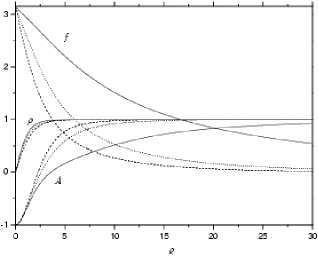
Figure 1: The D-type straight vortex with $n=1$ and $k=1$ which has $4\pi/g$ flux. Three solutions are shown: $\alpha=\beta=\gamma=0$ (solid lines), $\alpha=\beta=0$, $\gamma=0.005$ (dashed lines), and $\alpha=\gamma=0$, $\beta=-0.005$ (dotted lines). Here the unit of the scale is $1/{\bar{\rho}}$ and we have put $\lambda/g^{2}=2$.

The existence of two types of boundary conditions in two-gap superconductor has an important impact. To understand this notice that the magnetic flux of vortex is given by

$$\Phi=\oint A_{\mu}dx^{\mu}=\big{(}A(\infty)-A(0)\big{)}\displaystyle\frac{2\pi n}{g}.$$ (70)

Now, it is clear that the magnetic flux becomes fractional when $A(\infty)$ is fractional, which happens when $<n_{3}>\neq 1$ (or equivalently $<|\phi_{2}|>\neq 0$). As importantly, when $A(\infty)=1$ the magnetic flux becomes $2\pi(n+k)/g$ with $A(0)=-k/n$. This was impossible in ordinary superconductor. Now we classify the magnetic vortex in terms of the flux.

IV.1 $4\pi/g$-flux vortex

Let us choose the Dirichlet boundary condition at the core and the integer flux vacuum at the infinity ijpap ; cm2 . With $k=1$ we require

$$\rho(0)=0,~{}~{}\dot{\rho}(0)\neq 0,~{}~{}~{}\rho(\infty)=\sqrt{\displaystyle\frac{2(\mu+\gamma)}{(\lambda+\alpha+\beta)}},$$

$$f(0)=\pi,~{}~{}~{}~{}~{}f(\infty)=0,$$

$$A(0)=-\displaystyle\frac{1}{n},~{}~{}~{}~{}~{}A(\infty)=1.$$ (71)

With this we can integrate (63) to find the vortex solutions. The solutions with $n=1$ with different parameters are shown in Fig. 1. We call this a D-type vortex, because this comes from the Dirichlet boundary condition at the core. Both $\phi_{1}$ and $\phi_{2}$ start from zero at the core. However, notice that $\phi_{1}$ approaches the finite vacuum value but $\phi_{2}$ approaches zero at the infinity. So $\phi_{2}$ has a maximum concentration at a finite distance from the core. This is a generic feature of a D-type vortex.

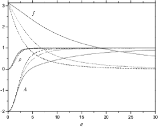
Figure 2: The D-type straight vortex with $n=1$ and $k=2$ which has $6\pi/g$ flux. Three solutions are shown: $\alpha=\beta=\gamma=0$ (solid lines), $\alpha=\beta=0$, $\gamma=0.005$ (dashed lines), and $\alpha=\gamma=0$, $\beta=-0.005$ (dotted lines). Here the unit of the scale is $1/{\bar{\rho}}$ and we have put $\lambda/g^{2}=2$.

With (71) the magnetic flux is given by

$$\Phi=\displaystyle\frac{}{}\int F_{\varrho\varphi}d^{2}x=\displaystyle\frac{}{}\int\partial_{\varrho}A_{\varphi}d^{2}x$$

$$=\Big{(}1+\displaystyle\frac{1}{n}\Big{)}\displaystyle\frac{2\pi n}{g}=\displaystyle\frac{2\pi}{g}(n+1),$$ (72)

so that when $n=1$ the vortex has $4\pi/g$ flux. Moreover, the solution has a non-Abelian topology. To see this notice that $\hat{n}$ defines a mapping $\pi_{2}(S^{2})=n$ from the compactifed $xy$-plane $S^{2}$ to the $CP^{1}$ space $S^{2}$. Clearly this is non-Abelian.

In general we may require

$$\rho(0)=\displaystyle\frac{d\rho}{d\varrho}(0)=...=\displaystyle\frac{d^{k-1}\rho}{d\varrho^{k-1}}(0)=0,$$

$$\displaystyle\frac{d^{k}\rho}{d\varrho^{k}}(0)\neq 0,~{}~{}~{}\rho(\infty)=\sqrt{\displaystyle\frac{2(\mu+\gamma)}{(\lambda+\alpha+\beta)}},$$

$$f(0)=\pi,~{}~{}~{}~{}~{}f(\infty)=0,$$

$$A(0)=-\displaystyle\frac{k}{n},~{}~{}~{}~{}~{}A(\infty)=1,$$ (73)

and obtain a different D-type vortex whose magnetic flux is given by

$$\Phi=\Big{(}1+\displaystyle\frac{k}{n}\Big{)}\displaystyle\frac{2\pi n}{g}=\displaystyle\frac{2\pi}{g}(n+k).$$ (74)

The $6\pi/g$-flux vortex with $n=1$ and $k=2$ is shown in Fig. 2. This tells that there exist infinitely many D-type vortices which have the same topology $\pi_{2}(S^{2})=n$. Again this is completely unexpected.

IV.2 $2\pi/g$-flux vortex

Now we choose the Neumann boundary condition at the core and the integer flux vacuum at the infinity ijpap ; cm2 ,

$$\rho(0)\neq 0,~{}~{}~{}\dot{\rho}(0)=0,~{}~{}~{}\rho(\infty)=\sqrt{\displaystyle\frac{2(\mu+\gamma)}{(\lambda+\alpha+\beta)}},$$

$$f(0)=\pi,~{}~{}~{}~{}~{}f(\infty)=0,$$

$$A(0)=0,~{}~{}~{}~{}~{}A(\infty)=1,$$ (75)

and find the vortex solutions. The solutions with $n=1$ but with different parameters are shown in Fig. 3. We call this a N-type vortex, because this comes from the Neumann boundary condition at the core. In this case $\phi_{1}$ behavior is the same as before. But notice that $\phi_{2}$ has a maximum concentration at the core, and approaches zero at the infinity. This is a generic feature of a N-type vortex.

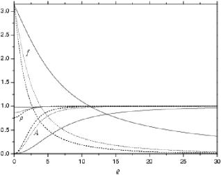
Figure 3: The N-type straight vortex with $n=1$ and $2\pi/g$ flux. Three solutions are shown: $\alpha=\beta=\gamma=0$ (solid lines), $\alpha=\beta=0$, $\gamma=0.005$ (dashed lines), and $\alpha=\gamma=0$, $\beta=-0.005$ (dotted lines). Here the unit of the scale is $1/{\bar{\rho}}$ and we have put $\lambda/g^{2}=2$.

The magnetic flux of the vortex is given by

$$\Phi=\displaystyle\frac{}{}\int F_{\varrho\varphi}d^{2}x=\displaystyle\frac{}{}\int\partial_{\varrho}A_{\varphi}d^{2}x$$

$$=\displaystyle\frac{2\pi n}{g},$$ (76)

so that it has the same flux as the Abrikosov vortex. But notice that the topology of the $CP^{1}$ field $\hat{n}$ is still non-Abelian as before, $\pi_{2}(S^{2})=n$. The reason why there exist two types of vortices which have different magnetic fluxes but have the same topology is that the magnetic flux is determined by the boundary condition $A(\infty)-A(0)$, not by the topology. The topology assures only the quantization of the flux, and does not determine what is the unit flux quantum.

IV.3 Fractional flux vortex

This is possible when we have the fractional flux vacuum at infinity

$$\rho(\infty)=2\sqrt{\displaystyle\frac{2\beta\mu-\alpha\gamma}{4\beta\lambda-\alpha^{2}}},~{}~{}~{}\cos f(\infty)=\displaystyle\frac{2\gamma\lambda-\alpha\mu}{2\beta\mu-\alpha\gamma},$$

$$A(\infty)=\displaystyle\frac{1}{2}\displaystyle\frac{2(\gamma\lambda+\beta\mu)-\alpha(\mu+\gamma)}{2\beta\mu-\alpha\gamma}.$$ (77)

At the core we can impose either the Dirichlet condition (66) or the Neumann condition (68).

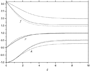
Figure 4: The D-type straight vortices with $n=1$ and $k=1$ which have a fractional flux with $\alpha=\gamma=0,~{}\beta=1.0$ (solid lines), $\alpha=0,~{}\beta=\lambda,~{}\gamma=-0.2$ (dashed lines), and $\alpha=-0.25,~{}\beta=\lambda,~{}\gamma=0$ (dotted lines). Here the unit of the scale is $1/{\bar{\rho}}$ and we have put $\lambda/g^{2}=2$.

We consider two special cases:
1. $\lambda_{11}=\lambda_{22}$ ($\alpha=0$). In this case we have

$$\rho(\infty)=\sqrt{\displaystyle\frac{2\mu}{\lambda}},~{}~{}~{}~{}\cos f(\infty)=\displaystyle\frac{\gamma\lambda}{\beta\mu}.$$ (78)

So with the Dirichlet boundary condition at the core the magnetic flux is given by

$$\Phi=\Big{(}\displaystyle\frac{\gamma\lambda}{2\beta\mu}+\displaystyle\frac{1}{2}+\displaystyle\frac{k}{n}\Big{)}\displaystyle\frac{2\pi n}{g},$$ (79)

but with the Neumann boundary condition at the core the magnetic flux is given by

$$\Phi=\Big{(}\displaystyle\frac{\gamma\lambda}{2\beta\mu}+\displaystyle\frac{1}{2}\Big{)}\displaystyle\frac{2\pi n}{g}.$$ (80)

Clearly they are fractional.
2. $\lambda_{12}=0$ ($\lambda=\beta$). In this case two condensates $\phi_{1}$ and $\phi_{2}$ have no direct coupling, and we have

$$<|\phi_{1}|>=\sqrt{\displaystyle\frac{\mu_{1}}{\lambda_{11}}},~{}~{}~{}~{}~{}<|\phi_{2}|>=\sqrt{\displaystyle\frac{\mu_{2}}{\lambda_{22}}}.$$ (81)

With this we have

$$\rho(\infty)=2\sqrt{\displaystyle\frac{2\lambda\mu-\alpha\gamma}{4\lambda^{2}-\alpha^{2}}},~{}~{}~{}\cos f(\infty)=\displaystyle\frac{2\gamma\lambda-\alpha\mu}{2\lambda\mu-\alpha\gamma},$$

$$A(\infty)=\displaystyle\frac{1}{2}\displaystyle\frac{(2\lambda-\alpha)(\mu+\gamma)}{2\mu\lambda-\alpha\gamma}.$$ (82)

So with the Dirichlet boundary condition at the core the magnetic flux is given by

$$\Phi=\Big{(}\displaystyle\frac{1}{2}\displaystyle\frac{(2\lambda-\alpha)(\mu+\gamma)}{2\lambda\mu-\alpha\gamma}+\displaystyle\frac{k}{n}\Big{)}\displaystyle\frac{2\pi n}{g},$$ (83)

but with the Neumann boundary condition at the core the magnetic flux is given by

$$\Phi=\displaystyle\frac{1}{2}\displaystyle\frac{(2\lambda-\alpha)(\mu+\gamma)}{2\lambda\mu-\alpha\gamma}\displaystyle\frac{2\pi n}{g}.$$ (84)

Again they are fractional, in spite of the fact that $\phi_{1}$ and $\phi_{2}$ have no direct coupling. This is because they are coupled through the electromagnetic potential, which tells that the two-gap superconductor is not a naive superposition of two one-gap superconductor.

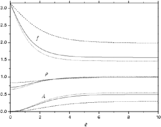
Figure 5: The N-type straight vortices with $n=1$ which have a fractional flux with $\alpha=\gamma=0,~{}\beta=1.0$ (solid lines), $\alpha=0,~{}\beta=\lambda,~{}\gamma=-0.2$ (dashed lines), and $\alpha=-0.25,~{}\beta=\lambda,~{}\gamma=0$ (dotted lines). Here the unit of the scale is $1/{\bar{\rho}}$ and we have put $\lambda/g^{2}=2$.

According to the different boundary condition at the core there are two types of fractional flux vortices, D-type and N-type. These fractional flux vortices with $n=1$ are plotted in Fig. 4 and Fig. 5. The fractional vortex is also topological, but the topology of the fractional vortex is different from that of integer flux vortex. Notice that for the fractional flux vortices the $\pi_{2}(S^{2})$ topology of $\hat{n}$ becomes trivial, $\pi_{2}(S^{2})=0$. This is because $\hat{n}$ does not cover the target space $S^{2}$ fully. But in this case we still have a $U(1)$ topology $\pi_{1}(S^{1})$, the topology of the $U(1)$ symmetry which leaves $\hat{n}$ invariant. And this Abelian topology describes the topology of the fractional flux vortex. So the topology of the fractional flux vortices is the same as that of the Abrikosov vortex.

An important feature of the fractional flux vortex is that the energy per unit length of the vortex is logarithmically divergent, which can be shown from the Hamiltonian (62). This is because the fractional flux vortex has a non-vanishing neutral current $k_{\mu}$ at the infinity. This, however, does not make the fractional flux vortex unphysical. In laboratory setting one can observe such vortex because one has a natural cutoff parameter $\Lambda$ fixed by the size of the superconductor, which can effectively make the energy of the fractional flux vortex finite. Indeed in $\rm He^{3}$ superfluid one often encounters the vorticity vortex whose energy is logarithmically divergent pra05 ; vol .

The existence of fractional flux vortices in two-gap superconductor has been pointed out before in London limit baba2 . Our analysis in this paper shows that the London limit does not fully describe the vortex in two-gap superconductor. This is because the magnetic flux is determined by the boundary condition at the origin (as well as the boundary condition at the infinity). Clearly the existence of two types of vortices which have different core structure and different magnetic flux can not be understood in London limit.

In this section we have shown that the two-gap superconductor can have totally different magnetic vortices which can not be found in ordinary superconductor. There are two types of vortices, D-type and N-type, and both have two different topologies, $\pi_{2}(S^{2})$ and $\pi_{1}(S^{1})$, which describe the vortices. The integral flux vortex is described by the $\pi_{2}(S^{2})$ topology, but the fractional vortex is described by the $\pi_{1}(S^{1})$ topology. As importantly, there are infinitely many different vortices within the same topological sector. Moreover, the magnetic flux of the D-type vortex is larger than that of the N-type vortex by a factor $2\pi k/g$, so that in the same topological sector the D-type vortex has more energy than the N-type vortex.

Obviously all these vortices are non-Abrikosov. This does not mean that two-gap superconductor can not admit an Abrikosov vortex. With $f=\pi$ (or $f=0$) and $\alpha=\beta=\gamma=0$, (63) describes an Abrikosov vortex. This is because with $\phi_{1}=0$ (or with $\phi_{2}=0$) the two-gap superconductor reduces to an ordinary superconductor.

V Helical vortex

In this section we show that the above non-Abrikosov vortices can be twisted to form a twisted magnetic vortex. With the twisting we obtain the helical vortex which is periodic in $z$-coordinate. To show this we choose the following ansatz ijpap ; cm2 ,

$$\rho=\rho(\varrho),~{}~{}~{}~{}~{}\xi=\left(\begin{array}[]{c}\cos\displaystyle\frac{f(\varrho)}{2}\exp(-in\varphi)\\ \sin\displaystyle\frac{f(\varrho)}{2}\exp(imkz)\end{array}\right),$$ (86)

$$A_{\mu}=\displaystyle\frac{1}{g}\Big{(}nA_{1}(\varrho)\partial_{\mu}\varphi+mkA_{2}(\varrho)\partial_{\mu}z\Big{)}.$$ (87)

Obviously the ansatz is periodic in $z$-coordinate, with the period $2\pi/k$.

With the ansatz we have

$$\hat{n}=\xi^{{\dagger}}\vec{\sigma}\xi=\left(\begin{array}[]{c}\sin f(\varrho)\cos(n\varphi+mkz)\\ \sin f(\varrho)\sin(n\varphi+mkz)\\ \cos f(\varrho)\end{array}\right),$$ (91)

$$C_{\mu}=n\displaystyle\frac{\cos{f(\varrho)}+1}{g}\partial_{\mu}\varphi+mk\displaystyle\frac{\cos{f(\varrho)}-1}{g}\partial_{\mu}z,$$

$$j_{\mu}=g\rho^{2}\Big{(}n\big{(}A_{1}-\displaystyle\frac{\cos{f}+1}{2}\big{)}\partial_{\mu}\varphi$$

$$+mk\big{(}A_{2}-\displaystyle\frac{\cos{f}-1}{2}\big{)}\partial_{\mu}z\Big{)},$$

$$k_{\mu}=g\rho^{2}\Big{(}n\big{(}A_{1}\cos f-\displaystyle\frac{\cos{f}+1}{2}\big{)}\partial_{\mu}\varphi$$

$$+mk\big{(}A_{2}\cos f+\displaystyle\frac{\cos{f}-1}{2}\big{)}\partial_{\mu}z\Big{)},$$ (92)

and the following Hamiltonian

$${\cal H}=\displaystyle\frac{1}{2}\dot{\rho}^{2}+\displaystyle\frac{1}{8}\rho^{2}\Big{(}\dot{f}^{2}+\big{(}\displaystyle\frac{n^{2}}{\varrho^{2}}+m^{2}k^{2}\big{)}\sin^{2}f\Big{)}$$

$$+\displaystyle\frac{\rho^{2}}{2}\Big{[}\displaystyle\frac{n^{2}}{\varrho^{2}}\Big{(}A_{1}-\displaystyle\frac{\cos f+1}{2}\Big{)}^{2}+m^{2}k^{2}\Big{(}A_{2}-\displaystyle\frac{\cos f-1}{2}\Big{)}^{2}\Big{]}$$

$$+\displaystyle\frac{1}{2g^{2}}\Big{(}\displaystyle\frac{n^{2}}{\varrho^{2}}\dot{A_{1}}^{2}+m^{2}k^{2}\dot{A_{2}}^{2}\Big{)}+\displaystyle\frac{\lambda}{8}\Big{[}(\rho^{2}-\bar{\rho}^{2})^{2}$$

$$+\displaystyle\frac{\alpha}{\lambda}(\rho^{2}-\displaystyle\frac{4\gamma}{\alpha})\rho^{2}\cos f+\displaystyle\frac{\beta}{\lambda}\rho^{4}\cos^{2}f\Big{]}-\displaystyle\frac{\mu^{2}}{2\lambda}.$$ (93)

With this (45) becomes

$$\ddot{\rho}+\displaystyle\frac{1}{\varrho}\dot{\rho}-\Big{[}\displaystyle\frac{1}{4}\big{(}\dot{f}^{2}+(\displaystyle\frac{n^{2}}{\varrho^{2}}+m^{2}k^{2})\sin^{2}f\big{)}$$

$$+\displaystyle\frac{n^{2}}{\varrho^{2}}(A_{1}-\displaystyle\frac{\cos{f}+1}{2})^{2}+m^{2}k^{2}(A_{2}-\displaystyle\frac{\cos{f}-1}{2})^{2}\Big{]}\rho$$

$$=\displaystyle\frac{\lambda}{2}\Big{[}\big{(}\rho^{2}-\rho_{0}^{2}\big{)}+\displaystyle\frac{\alpha}{\lambda}\big{(}\rho^{2}-\displaystyle\frac{2\gamma}{\alpha}\big{)}\cos f+\displaystyle\frac{\beta}{\lambda}\rho^{2}\cos^{2}f\Big{]}\rho,$$

$$\ddot{f}+\big{(}\displaystyle\frac{1}{\varrho}+2\displaystyle\frac{\dot{\rho}}{\rho}\big{)}\dot{f}-2\Big{[}\displaystyle\frac{n^{2}}{\varrho^{2}}\big{(}A_{1}-\displaystyle\frac{1}{2}\big{)}$$

$$+m^{2}k^{2}\big{(}A_{2}+\displaystyle\frac{1}{2}\big{)}\Big{]}\sin f$$

$$=\Big{(}2\gamma-\big{(}\displaystyle\frac{\alpha}{2}+\beta\cos f\big{)}\rho^{2}\Big{)}\sin f,$$

$$\ddot{A_{1}}-\displaystyle\frac{1}{\varrho}\dot{A}_{1}-g^{2}\rho^{2}\Big{(}A_{1}-\displaystyle\frac{\cos{f}+1}{2}\Big{)}=0,$$

$$\ddot{A_{2}}+\displaystyle\frac{1}{\varrho}\dot{A}_{2}-g^{2}\rho^{2}\Big{(}A_{2}-\displaystyle\frac{\cos{f}-1}{2}\Big{)}=0.$$ (94)

This is an obvious generalization of (63).

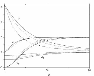
Figure 6: The D-type helical vortex with $4\pi/g$-flux along the vortex with $m=n=1$ (with $k=1$). Three solutions are shown: $\alpha=\beta=\gamma=0$ (solid lines), $\alpha=\beta=0$ and $\gamma=0.005$ (dashed lines), $\alpha=\gamma=0$ and $\beta=-0.005$ (dotted lines). Here the unit of the scale is $1/{\bar{\rho}}$ and we have put $k=0.12\bar{\rho}$ and $\lambda/g^{2}=2$.

To obtain the helical vortex we first consider the integer flux boundary condition at the infinity

$$\rho(\infty)=\sqrt{\displaystyle\frac{2(\mu+\gamma)}{(\lambda+\beta+\alpha)}},~{}~{}~{}~{}~{}f(\infty)=0,$$

$$A_{1}(\infty)=1,~{}~{}~{}~{}~{}A_{2}(\infty)=0.$$ (95)

Just like the straight vortex, there are two types of boundary conditions at the core. Here we consider only the case $n=1$ for simplicity:
A. Dirichlet boundary condition

$$\rho(0)=0,~{}~{}~{}~{}~{}f(0)=\pi,$$

$$A_{1}(0)=-1,~{}~{}~{}~{}~{}\dot{A}_{2}(0)=0.$$ (96)

B. Neumann boundary condition

$$\dot{\rho}(0)=0,~{}~{}~{}~{}~{}f(0)=\pi,$$

$$A_{1}(0)=0,~{}~{}~{}~{}~{}\dot{A}_{2}(0)=0.$$ (97)

With the Dirichlet boundary condition we have the D-type helical vortex which has $4\pi/g$-flux along the vortex shown in Fig. 6, but with the Neumann boundary condition we have the N-type helical vortex which has $2\pi/g$-flux along the vortex shown in Fig. 7.

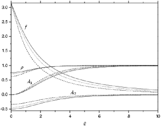
Figure 7: The N-type helical vortex with $2\pi/g$-flux along the vortex with $m=n=1$. Three solutions are shown: $\alpha=\beta=\gamma=0$ (solid lines), $\alpha=\beta=0$ and $\gamma=0.005$ (dashed lines), $\alpha=\gamma=0$ and $\beta=-0.005$ (dotted lines). Here the unit of the scale is $1/{\bar{\rho}}$ and we have put $k=0.12\bar{\rho}$ and $\lambda/g^{2}=2$.

For the fractional flux helical vortex we impose the fractional flux boundary condition at the infinity

$$\rho(\infty)=2\sqrt{\displaystyle\frac{2\beta\mu-\alpha\gamma}{4\beta\lambda-\alpha^{2}}},~{}~{}~{}\cos f(\infty)=\displaystyle\frac{2\gamma\lambda-\alpha\mu}{2\beta\mu-\alpha\gamma},$$

$$A_{1}(\infty)=\displaystyle\frac{1}{2}\displaystyle\frac{2(\gamma\lambda+\beta\mu)-\alpha(\mu+\gamma)}{2\beta\mu-\alpha\gamma},$$

$$A_{2}(\infty)=\displaystyle\frac{1}{2}\displaystyle\frac{2(\gamma\lambda-\beta\mu)-\alpha(\mu-\gamma)}{2\beta\mu-\alpha\gamma}.$$

Now, with the Dirichlet boundary condition at the core, we obtain the D-type helical vortex which has a fractional flux along the vortex shown in Fig. 8. But with the Neumann boundary condition (97) at the core, we obtain the N-type helical vortex which has a fractional flux along the vortex shown in Fig. 9. Notice that, just as the fractional flux straight vortex, the energy per one period of the fractional flux helical vortex is logarithmically divergent.

A new feature of the helical vortex is that the magnetic flux becomes helical. Indeed the ansatz (87) tells that the magnetic flux can be decomposed to the one along the vortex and the other around the vortex ijpap ; cm2

$$F_{\hat{\varrho}\hat{\varphi}}=\displaystyle\frac{n}{g}\displaystyle\frac{\dot{A}_{1}}{\varrho},~{}~{}~{}F_{\hat{z}\hat{\varrho}}=-\displaystyle\frac{mk}{g}\dot{A}_{2},$$ (98)

so that we have two magnetic fluxes linked together,

$$\Phi_{\hat{z}}=\displaystyle\frac{}{}\int F_{\hat{\varrho}\hat{\varphi}}\varrho d\varrho d\varphi=\Big{(}A_{1}(\infty)-A_{1}(0)\Big{)}\displaystyle\frac{2\pi n}{g},$$

$$\Phi_{\hat{\varphi}}=\displaystyle\frac{}{}\int F_{\hat{z}\hat{\varrho}}dzd\varrho=-\Big{(}A_{2}(\infty)-A_{2}(0)\Big{)}\displaystyle\frac{2\pi m}{g}.$$ (99)

Obviously $\Phi_{\hat{\varphi}}$ is due to the helical structure of the vortex, which becomes fractional in general.

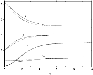
Figure 8: The D-type helical vortices which have a fractional flux with $m=n=1$ (with $k=1$). Two solutions with $\alpha=\gamma=0,~{}\beta=0.5$ (solid lines), and $\alpha=\gamma=0,~{}\beta=1.0$ (dashed lines) are shown. Here the unit of the scale is $1/{\bar{\rho}}$ and we have put $\lambda/g^{2}=2,~{}k=0.1\bar{\rho}$.

Another important feature of the helical vortex is that the electromagnetic current $j_{\mu}$ which is responsible for the Meissner effect also becomes helical. In particular, it has a non-trivial electromagnetic current $j_{\hat{z}}$ along the vortex which generates the magnetic flux $\Phi_{\hat{\varphi}}$, in addition to the usual electromagnetic current $j_{\hat{\varphi}}$ around the vortex which is responsible for $\Phi_{\hat{z}}$. But notice that the total electromagnetic current $i_{\hat{z}}$ along the vortex becomes zero. This, together with (61), tells that $\phi_{1}$ and $\phi_{2}$ generate non-vanishing electromagnetic currents $i_{\hat{z}}^{(1)}$ and $i_{\hat{z}}^{(2)}$ which flow oppositely and cancel each other. In this sense we may call the helical vortex superconducting, even though it has no net electromagnetic current $i_{\hat{z}}$ along the vortex ijpap ; cm2 .

VI magnetic knot in two-gap superconductor

Clearly the helical vortex is unstable unless the periodicity condition is enforced by hand. Nevertheless it has an important implication, because the helical vortex predicts the existence of a topological knot in two-gap superconductor. This is because we can make it a twisted magnetic vortex ring smoothly bending and connecting two periodic ends together. The resulting twisted magnetic vortex ring becomes a knot whose topology is described by the Chern-Simon index of the electromagnetic potential ijpap ; cm2 .

There have been two objections against the existence of a stable magnetic vortex ring in Abelian superconductor. First, it is supposed to be unstable due to the tension created by the ring huang . Indeed if one constructs a vortex ring from an Abrikosov vortex, it becomes unstable because of the tension. But we can easily overcome this difficulty by twisting the magnetic vortex first and connecting the periodic ends together. In this case the non-trivial twist of the magnetic field forbids the untwisting of the vortex ring by any smooth deformation of field configuration, and the vortex ring becomes a stable knot. The other objection is that the Abelian gauge theory is supposed to have no non-trivial knot topology which allows a stable vortex ring. This again is a common misconception. As we have seen, the theory has a well-defined knot topology $\pi_{3}(S^{2})$ described by the Chern-Simon index of the electromagnetic potential. This tells that there is no reason whatsoever why the Abelian superconductor can not have a topological knot.

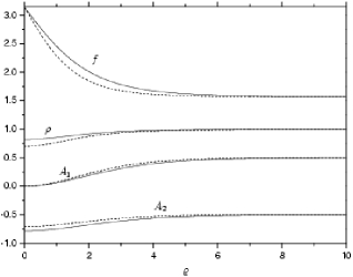
Figure 9: The N-type helical vortices which have a fractional flux with $m=n=1$. Two solutions with $\alpha=\gamma=0,~{}\beta=0.5$ (solid lines), and $\alpha=\gamma=0,~{}\beta=1.0$ (dashed lines) are shown. Here the unit of the scale is $1/{\bar{\rho}}$ and we have put $\lambda/g^{2}=2,~{}k=0.1\bar{\rho}$.

To demonstrate the existence of a topological knot in the two-gap superconductor, we introduce the toroidal coordinates ($\eta,\gamma,\varphi$) defined by

$$x=\displaystyle\frac{a}{D}\sinh{\eta}\cos{\varphi},~{}~{}~{}y=\displaystyle\frac{a}{D}\sinh{\eta}\sin{\varphi},$$

$$z=\displaystyle\frac{a}{D}\sin{\gamma},$$

$$D=\cosh{\eta}-\cos{\gamma},$$

$$ds^{2}=\displaystyle\frac{a^{2}}{D^{2}}\Big{(}d\eta^{2}+d\gamma^{2}+\sinh^{2}\eta d\varphi^{2}\Big{)},$$

$$d^{3}x=\displaystyle\frac{a^{3}}{D^{3}}\sinh{\eta}d\eta d\gamma d\varphi,$$ (100)

where $a$ is the radius of the knot defined by $\eta=\infty$. Notice that in toroidal coordinates, $\eta=\gamma=0$ represents spatial infinity of $R^{3}$, and $\eta=\infty$ describes the torus center.

Now we choose the following ansatz,

$$\phi=\displaystyle\frac{1}{\sqrt{2}}\rho(\eta,\gamma)\Bigg{(}\matrix{\cos\displaystyle\frac{f(\eta,\gamma)}{2}\exp(-im\varphi)\cr\sin\displaystyle\frac{f(\eta,\gamma)}{2}\exp(in\omega(\eta,\gamma))}\Bigg{)},$$

$$A_{\mu}=\displaystyle\frac{n}{g}A_{0}(\eta,\gamma)\partial_{\mu}\eta+\displaystyle\frac{n}{g}A_{1}(\eta,\gamma)\partial_{\mu}\gamma$$

$$+\displaystyle\frac{m}{g}A_{2}(\eta,\gamma)\partial_{\mu}\varphi.$$ (101)

With this we have

$$\hat{n}=\Bigg{(}\matrix{\sin f(\eta,\gamma)\cos(n\omega+m\varphi)\cr\sin f(\eta,\gamma)\sin(n\omega+m\varphi)\cr\cos f(\eta,\gamma)}\Bigg{)},$$

$$C_{\mu}=\displaystyle\frac{m}{2g}(\cos f+1)\partial_{\mu}\varphi+\displaystyle\frac{n}{2g}(\cos f-1)\partial_{\mu}\omega,$$

$$F_{\eta\gamma}=\displaystyle\frac{n}{g}\big{(}\partial_{\eta}A_{1}-\partial_{\gamma}A_{0}\big{)},$$

$$F_{\gamma\varphi}=\displaystyle\frac{m}{g}\partial_{\gamma}A_{2},~{}~{}~{}~{}~{}F_{\varphi\eta}=-\displaystyle\frac{m}{g}\partial_{\eta}A_{2}.$$ (102)

Notice that, in the orthonormal frame $(\hat{\eta},\hat{\gamma},\hat{\varphi})$, we have

$$A_{\hat{\eta}}=\displaystyle\frac{D}{a}A_{\eta},~{}~{}A_{\hat{\gamma}}=\displaystyle\frac{D}{a}A_{\gamma},~{}~{}A_{\hat{\varphi}}=\displaystyle\frac{D}{a\sinh\eta}A_{\varphi},$$

$$F_{\hat{\eta}\hat{\gamma}}=\displaystyle\frac{nD^{2}}{ga^{2}}\big{(}\partial_{\eta}A_{1}-\partial_{\gamma}A_{0}\big{)},$$

$$F_{\hat{\gamma}\hat{\varphi}}=\displaystyle\frac{mD^{2}}{ga^{2}\sinh\eta}\partial_{\gamma}A_{2},$$

$$F_{\hat{\varphi}\hat{\eta}}=-\displaystyle\frac{mD^{2}}{ga^{2}\sinh\eta}\partial_{\eta}A_{2}.$$

Next, we adopt the $SU(2)$ symmetric potential with $\lambda_{11}=\lambda_{22}=\lambda_{12}=\lambda$ and $\mu_{1}=\mu_{2}=\mu$ for simplicity. In this case we have the following knot equation

$$\Bigg{[}\partial_{\eta}^{2}+\partial_{\gamma}^{2}+\Big{(}\displaystyle\frac{\cosh\eta}{\sinh\eta}-\displaystyle\frac{\sinh\eta}{D}\Big{)}\partial_{\eta}-\displaystyle\frac{\sin\gamma}{D}\partial_{\gamma}\Bigg{]}\rho-\displaystyle\frac{1}{4}\Bigg{[}\big{(}\partial_{\eta}f\big{)}^{2}+\big{(}\partial_{\gamma}f\big{)}^{2}$$

$$+\sin^{2}f\Big{(}n^{2}\big{(}\partial_{\eta}\omega\big{)}^{2}+n^{2}\big{(}\partial_{\gamma}\omega\big{)}^{2}+\displaystyle\frac{m^{2}}{\sinh^{2}\eta}\Big{)}\Bigg{]}\rho-\Bigg{[}n^{2}\Big{(}A_{0}-\displaystyle\frac{\cos f+1}{2}\partial_{\eta}\omega\Big{)}^{2}+n^{2}\Big{(}A_{1}-\displaystyle\frac{\cos f+1}{2}\partial_{\gamma}\omega\Big{)}^{2}$$

$$+\displaystyle\frac{m^{2}}{\sinh^{2}\eta}\Big{(}A_{2}-\displaystyle\frac{\cos f-1}{2}\Big{)}^{2}\Bigg{]}\rho=\displaystyle\frac{\lambda}{2}\displaystyle\frac{a^{2}}{D^{2}}\Big{(}\rho^{2}-\bar{\rho}^{2}\Big{)}\rho,$$

$$\Bigg{[}\partial_{\eta}^{2}+\partial_{\gamma}^{2}+\Big{(}\displaystyle\frac{\cosh\eta}{\sinh\eta}-\displaystyle\frac{\sinh\eta}{D}\Big{)}\partial_{\eta}-\displaystyle\frac{\sin\gamma}{D}\partial_{\gamma}\Bigg{]}f+\displaystyle\frac{2}{\rho}\Big{(}\partial_{\eta}f\partial_{\eta}\rho+\partial_{\gamma}f\partial_{\gamma}\rho\Big{)}$$

$$=2\sin f\Bigg{[}n^{2}\Big{(}A_{0}-\displaystyle\frac{1}{2}\partial_{\eta}\omega\Big{)}\partial_{\eta}\omega+n^{2}\Big{(}A_{1}-\displaystyle\frac{1}{2}\partial_{\gamma}\omega\Big{)}\partial_{\gamma}\omega+\displaystyle\frac{m^{2}}{\sinh^{2}\eta}\Big{(}A_{2}+\displaystyle\frac{1}{2}\Big{)}\Bigg{]},$$

$$\Bigg{[}\partial_{\eta}^{2}+\partial_{\gamma}^{2}+\Big{(}\displaystyle\frac{\cosh\eta}{\sinh\eta}-\displaystyle\frac{\sinh\eta}{D}\Big{)}\partial_{\eta}-\displaystyle\frac{\sin\gamma}{D}\partial_{\gamma}\Bigg{]}\omega+\displaystyle\frac{2}{\rho}\Big{(}\partial_{\eta}\rho\partial_{\eta}\omega+\partial_{\gamma}\rho\partial_{\gamma}\omega\Big{)}-\displaystyle\frac{\sin f}{1+\cos f}\Big{(}\partial_{\eta}f\partial_{\eta}\omega+\partial_{\gamma}f\partial_{\gamma}\omega\Big{)}$$

$$+\displaystyle\frac{2}{\sin f}\Big{(}\partial_{\eta}fA_{0}+\partial_{\gamma}fA_{1}\Big{)}=0,$$

$$\Big{(}\partial_{\gamma}+\displaystyle\frac{\sin\gamma}{D}\Big{)}\Big{(}\partial_{\gamma}A_{0}-\partial_{\eta}A_{1}\Big{)}=\displaystyle\frac{a^{2}}{D^{2}}g^{2}\rho^{2}\Big{(}A_{0}-\displaystyle\frac{\cos f+1}{2}\partial_{\eta}\omega\Big{)},$$

$$\Big{(}\partial_{\eta}+\displaystyle\frac{\cosh\eta}{\sinh\eta}+\displaystyle\frac{\sinh\eta}{D}\Big{)}\Big{(}\partial_{\eta}A_{1}-\partial_{\gamma}A_{0}\Big{)}=\displaystyle\frac{a^{2}}{D^{2}}g^{2}\rho^{2}\Big{(}A_{1}-\displaystyle\frac{\cos f+1}{2}\partial_{\gamma}\omega\Big{)},$$

$$\Bigg{[}\partial_{\eta}^{2}+\partial_{\gamma}^{2}-\Big{(}\displaystyle\frac{\cosh\eta}{\sinh\eta}-\displaystyle\frac{\sinh\eta}{D}\Big{)}\partial_{\eta}+\displaystyle\frac{\sin\gamma}{D}\partial_{\gamma}\Bigg{]}A_{2}=\displaystyle\frac{a^{2}}{D^{2}}g^{2}\rho^{2}\Big{(}A_{2}-\displaystyle\frac{\cos f-1}{2}\Big{)}.$$ (103)

Moreover, from (4) and (101) we have the following Hamiltonian for the knot

$${\cal H}=\displaystyle\frac{D^{2}}{2a^{2}}\Bigg{[}(\partial_{\eta}\rho)^{2}+(\partial_{\gamma}\rho)^{2}+\displaystyle\frac{1}{4}\rho^{2}\big{(}(\partial_{\eta}f)^{2}+(\partial_{\gamma}f)^{2}\big{)}+\displaystyle\frac{1}{4}\rho^{2}\sin^{2}f\Big{(}n^{2}(\partial_{\eta}\omega)^{2}+n^{2}(\partial_{\gamma}\omega)^{2}+\displaystyle\frac{m^{2}}{\sinh^{2}\eta}\Big{)}\Bigg{]}$$

$$+\displaystyle\frac{D^{2}}{2a^{2}}\Bigg{[}n^{2}(A_{0}-\displaystyle\frac{\cos f+1}{2}\partial_{\eta}\omega)^{2}+n^{2}(A_{1}-\displaystyle\frac{\cos f+1}{2}\partial_{\gamma}\omega)^{2}+\displaystyle\frac{m^{2}}{\sinh^{2}\eta}(A_{2}-\displaystyle\frac{\cos f-1}{2})^{2}\Bigg{]}\rho^{2}$$

$$+\displaystyle\frac{D^{4}}{2g^{2}a^{4}}\Bigg{[}n^{2}(\partial_{\eta}A_{1}-\partial_{\gamma}A_{0})^{2}+\displaystyle\frac{m^{2}}{\sinh^{2}\eta}\Big{(}(\partial_{\eta}A_{2})^{2}+(\partial_{\gamma}A_{2})^{2}\Big{)}\Bigg{]}+\displaystyle\frac{\lambda}{8}(\rho^{2}-\bar{\rho}^{2})^{2}.$$ (104)

Minimizing the energy we reproduce the knot equation (103).

In toroidal coordinates, $\eta=\gamma=0$ represents spatial infinity of $R^{3}$, and $\eta=\infty$ describes the torus center. So we can impose the following Neumann boundary condition

$$\rho(0,0)=\bar{\rho},~{}~{}~{}~{}~{}\dot{\rho}(\infty,\gamma)=0,$$

$$f(0,\gamma)=0,~{}~{}~{}~{}~{}f(\infty,\gamma)=\pi,$$

$$\omega(\eta,0)=0,~{}~{}~{}~{}~{}\omega(\eta,2\pi)=2\pi,$$

$$A_{0}(0,\gamma)=0,~{}~{}~{}~{}~{}A_{0}(\infty,\gamma)=0,$$

$$A_{1}(0,\gamma)=1,~{}~{}~{}~{}~{}A_{1}(\infty,\gamma)=0,$$

$$A_{2}(0,\gamma)=0,~{}~{}~{}~{}~{}A_{2}(\infty,\gamma)=-1,$$ (105)

to obtain the desired knot. A numerical integration of (103) with the boundary conditions (105) is difficult to perform. But we can obtain the actual knot profile of $\rho,~{}f$, and $\omega$ by minimizing the energy. From (104) the knot energy is given by

$$E=\displaystyle\frac{}{}\int{\cal H}\displaystyle\frac{a^{3}}{D^{3}}\sinh\eta d\eta d\gamma d\varphi.$$ (106)

We find that, for $m=n=1$, the radius of knot which minimizes the energy (106) is given by

$$a\simeq\displaystyle\frac{1.2}{\sqrt{2\mu}}.$$ (107)

From this we obtain the three-dimensional energy profile of the lightest axially symmetric knot in two-gap superconductor, which is shown in Fig. 10.

With this we can estimate the energy of the axially symmetric knot,

$$E\simeq 51\displaystyle\frac{\bar{\rho}}{\sqrt{\lambda}}.$$ (108)

We can also calculate the magnetic flux of the knot. Since the flux is helical, we have two fluxes, the flux $\Phi_{\hat{\gamma}}$ passing through the knot disk of radius $a$ in the $xy$-plane and the flux $\Phi_{\hat{\varphi}}$ which surrounds it. From the knot solution we find

$$\Phi_{\hat{\eta}}=\displaystyle\frac{}{}\int F_{\gamma\varphi}d\gamma d\varphi=0.$$

$$\Phi_{\hat{\gamma}}=\displaystyle\frac{}{}\int F_{\varphi\eta}d\varphi d\eta=\displaystyle\frac{2m\pi}{g},$$

$$\Phi_{\hat{\varphi}}=\displaystyle\frac{}{}\int F_{\eta\gamma}d\eta d\gamma=-\displaystyle\frac{2n\pi}{g}$$ (109)

The flux is quantized in the unit of $2\pi/g$, but this is due to the $SU(2)$ symmetric potential and the Neumann boundary condition (105). In general they can be fractional. But independent of this the two fluxes are linked, whose linking number becomes $mn$. This is important.

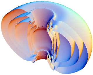
Figure 10: The energy profile of a N-type knot with $m=n=1$. Here we have put $\lambda/g^{2}=2$.

This confirms that the knot can be viewed as a twisted magnetic vortex ring, where the linking of two magnetic fluxes provides the knot topology. There is a natural candidate which can describe this topology of twisted magnetic vortex ring, the Chern-Simon index of the electromagnetic potential which describes the $\pi_{3}(S^{2})$ topology. We can calculate the knot quantum number from the Chern-Simon index, and find

$$Q_{CS}=-\displaystyle\frac{mn}{8\pi^{2}}\int\varepsilon^{ijk}A_{i}F_{jk}dx^{3}=mn.$$ (110)

This confirms that the Chern-Simon index is indeed given by the linking number of two magnetic fluxes $\Phi_{\hat{\gamma}}$ and $\Phi_{\hat{\varphi}}$.

It has been asserted that the knot topology is described by the $\pi_{3}(S^{2})$ topology of the $CP^{1}$ field $\hat{n}$ baba1 . We emphasize that this is only partially true, which becomes correct only when the knot carries an integer magnetic flux. Indeed, in this case $\hat{n}$ acquires a non-trivial knot topology $\pi_{3}(S^{2})$, which is given by ijpap

$$Q=-\displaystyle\frac{mn}{8\pi^{2}}\int(\partial_{\eta}f\partial_{\gamma}\omega-\partial_{\gamma}f\partial_{\eta}\omega)\sin fd\eta d\gamma d\varphi$$

$$=-\displaystyle\frac{mn}{4\pi}\int\sin fdfd\omega=mn,$$ (111)

where the last equality comes from the boundary condition (105). Notice, however, that the $\pi_{3}(S^{2})$ topology of $\hat{n}$ becomes trivial when the knot has a fractional flux. This is because the fractional flux knot comes from a fractional flux vortex, which has a trivial $\pi_{2}(S^{2})$ topology. This means that the $\pi_{3}(S^{2})$ topology of $\hat{n}$ can not describe the topology of a fractional flux knot. In contrast, the Chern-Simon index of the electromagnetic potential can still provide the non-trivial $\pi_{3}(S^{2})$, even when the knot has a fractional flux. This is because the Chern-Simon index describes the knot topology of the twisted magnetic flux.

VII Josephson Interaction

It has been well-known that two-gap superconductor may allow the prototype Josephson interaction maz

$$\eta(\phi_{1}^{*}\phi_{2}+\phi_{1}\phi_{2}^{*}),$$ (112)

where $\eta$ is a coupling constant. But we can consider a more general quartic Josephson interaction,

$$V_{J}=\bar{\eta}\Big{[}\big{(}\phi_{1}^{*}\phi_{2}\exp(i\theta_{1})+\phi_{2}^{*}\phi_{1}\exp(-i\theta_{1})\big{)}\Big{]}$$

$$+\bar{\eta}_{1}\Big{[}(\phi_{1}^{*}\phi_{2})^{2}\exp(i\theta_{2})+(\phi_{2}^{*}\phi_{1})^{2}\exp(-i\theta_{2})\Big{]}$$

$$+\bar{\eta}_{2}(|\phi_{1}|^{2}+|\phi_{2}|^{2})\Big{[}\big{(}\phi_{1}^{*}\phi_{2}\exp(i\theta_{3})+\phi_{2}^{*}\phi_{1}exp(-i\theta_{3})\big{)}\Big{]}$$

$$+\bar{\eta}_{3}(|\phi_{1}|^{2}-|\phi_{2}|^{2})\Big{[}\big{(}\phi_{1}^{*}\phi_{2}\exp(i\theta_{4})$$

$$+\phi_{2}^{*}\phi_{1}\exp(-i\theta_{4})\big{)}\Big{]}.$$ (113)

Clearly the Josephson interaction breaks the $U(1)\times U(1)$ symmetry of the potential (5) down to $U(1)$. In general it is not easy to accommodate this type of generalized Josephson interaction. But for simpler Josephson interactions we can accommodate them within the framework of the potential (5). To understand how, notice that the potential (5) already has a Josephson interaction in the sense that it allows an interband transition between $\phi_{1}$ and $\phi_{2}$ when $\lambda_{12}$ is not zero. This implies that the above Josephson interaction could be included in the $\lambda_{12}$ interaction.

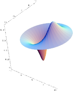
(a)   $|\phi_{1}|^{2}$

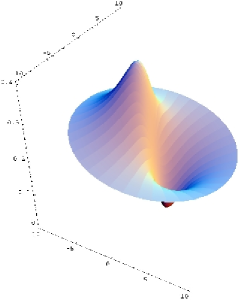
(b)   $|\phi_{2}|^{2}$

Figure 11: The density profile of $|\phi_{1}|^{2}$ and $|\phi_{2}|^{2}$ of the N-type magnetic vortex in the presence of Josephson interaction. Here we have put $\bar{\rho}=1$, $\gamma=0.05$, $\eta=0.25$, and $\lambda/g^{2}=2$.

To exploit this point we generalize the $U(1)\times U(1)$ symmetric potential (5) to

$$V\rightarrow\bar{V}=V+V_{1},$$

$$V_{1}=\eta\Big{[}\big{(}\phi_{1}^{*}\phi_{2}\exp(i\theta)+\phi_{2}^{*}\phi_{1}\exp(-i\theta)\big{)}\Big{]}$$

$$+\eta_{1}\Big{[}\big{(}\phi_{1}^{*}\phi_{2})^{2}\exp(2i\theta)+(\phi_{2}^{*}\phi_{1})^{2}\exp(-2i\theta)\big{)}\Big{]}$$

$$+\eta_{2}(|\phi_{1}|^{2}+|\phi_{2}|^{2})\Big{[}\big{(}\phi_{1}^{*}\phi_{2}\exp(i\theta)+\phi_{2}^{*}\phi_{1}\exp(-i\theta)\big{)}\Big{]}$$

$$+\eta_{3}(|\phi_{1}|^{2}-|\phi_{2}|^{2})\Big{[}\big{(}\phi_{1}^{*}\phi_{2}\exp(i\theta)$$

$$+\phi_{2}^{*}\phi_{1}\exp(-i\theta)\big{)}\Big{]},$$ (114)

and introduce a new doublet $\psi$ with an $SU(2)$ transformation of $\phi$,

$$\psi={\cal M}\phi,$$

$${\cal M}=\Bigg{(}\matrix{\cos\displaystyle\frac{a}{2}\exp(ib)~{}~{}~{}-\sin\displaystyle\frac{a}{2}\exp(ic)\cr\sin\displaystyle\frac{a}{2}\exp(-ic)~{}~{}\cos\displaystyle\frac{a}{2}\exp(-ib)}\Bigg{)},$$

$$\tan a=\displaystyle\frac{\eta}{\gamma}.$$ (115)

Now, we can show that when

$$\theta=-b+c,$$

$$\eta_{1}=\displaystyle\frac{\eta^{2}}{2\gamma^{2}-\eta^{2}}\beta,~{}~{}~{}~{}\eta_{2}=-\displaystyle\frac{\eta}{2\gamma}\alpha,$$

$$\eta_{3}=\displaystyle\frac{2\gamma\eta}{2\gamma^{2}-\eta^{2}}\beta,$$ (116)

the potential (114) can be written as

$$\bar{V}=\displaystyle\frac{\lambda_{11}^{\prime}}{2}|\psi_{1}|^{4}+\lambda_{12}^{\prime}|\psi_{1}|^{2}|\psi_{2}|^{2}+\displaystyle\frac{\lambda_{22}^{\prime}}{2}|\psi_{2}|^{4}$$

$$-\mu_{1}^{\prime}|\psi_{1}|^{2}-\mu_{2}^{\prime}|\psi_{2}|^{2}$$

$$=\displaystyle\frac{\lambda^{\prime}}{2}(|\psi_{1}|^{2}+|\psi_{2}|^{2}-\displaystyle\frac{\mu^{\prime}}{\lambda^{\prime}})^{2}+\displaystyle\frac{\alpha^{\prime}}{2}(|\psi_{1}|^{4}-|\psi_{2}|^{4})$$

$$+\displaystyle\frac{\beta^{\prime}}{2}(|\psi_{1}|^{2}-|\psi_{2}|^{2})^{2}-\gamma^{\prime}(|\psi_{1}|^{2}-|\psi_{2}|^{2})$$

$$-\displaystyle\frac{\mu^{\prime}}{2\lambda^{\prime}},$$ (117)

where

$$\lambda^{\prime}=\lambda-\eta_{1},$$

$$\alpha^{\prime}=\displaystyle\frac{\sqrt{\gamma^{2}+\eta^{2}}}{\gamma}\alpha,~{}~{}~{}\beta^{\prime}=\displaystyle\frac{2(\gamma^{2}+\eta^{2})}{2\gamma^{2}-\eta^{2}}\beta,$$

$$\mu^{\prime}=\mu,~{}~{}~{}~{}~{}\gamma^{\prime}=\sqrt{\gamma^{2}+\eta^{2}}.$$ (118)

So in terms of $\psi_{1}$ and $\psi_{2}$ the potential (114) becomes the potential (39) which has no Josephson interaction. This means that, with (116), we can formally absorb the Josephson interaction to $\lambda_{12}$ interaction. From this we concludes that the presence of the Josephson interaction does not affect the existence of the topological objects in two-gap superconductor.

This does not mean that the Josephson interaction does not affect the topological solutions. On the contrary, it does change the shape of the solutions drastically. This is because under the transformation (115) the profile of $\phi_{1}$ and $\phi_{2}$ change drastically. To demonstrate this we let $\alpha=\beta=0$ for simplicity, and adopt the potential which has the following Josephson interaction

$$V=\displaystyle\frac{\lambda}{2}(|\phi_{1}|^{2}+|\phi_{2}|^{2}-\displaystyle\frac{\mu}{\lambda})^{2}-\gamma(|\phi_{1}|^{2}-|\phi_{2}|^{2})$$

$$+\eta(\phi_{1}^{*}\phi_{2}\exp(i\theta)+\phi_{1}\phi_{2}^{*}\exp(-i\theta)).$$ (119)

Notice that, in terms of $\psi$, the potential is written as

$$V=\displaystyle\frac{\lambda}{2}(|\psi_{1}|^{2}+|\psi_{2}|^{2}-\displaystyle\frac{\mu}{\lambda})^{2}$$

$$-\sqrt{\gamma^{2}+\eta^{2}}(|\phi_{1}|^{2}-|\phi_{2}|^{2}),$$ (120)

so that it clearly has two types of straight vortex solution of the following form

$$\psi=\displaystyle\frac{\rho}{\sqrt{2}}\Bigg{(}\matrix{\cos\displaystyle\frac{f}{2}\exp(-in\varphi)\cr\sin\displaystyle\frac{f}{2}}\Bigg{)},~{}~{}~{}\rho=\rho(\varrho),$$

$$A_{\mu}=\displaystyle\frac{n}{g}A(\varrho)\partial_{\mu}\varphi.$$ (121)

Now, in terms of $\phi$, the solution acquires the form

$$\phi=\displaystyle\frac{\rho}{\sqrt{2}}\Big{(}\matrix{\xi_{1}\cr\xi_{2}}\Big{)},$$

$$\xi_{1}=\cos\displaystyle\frac{f}{2}\cos\displaystyle\frac{a}{2}\exp(-in\varphi-ib)$$

$$+\sin\displaystyle\frac{f}{2}\sin\displaystyle\frac{a}{2}\exp(i\theta+ib),$$

$$\xi_{2}=-\cos\displaystyle\frac{f}{2}\sin\displaystyle\frac{a}{2}\exp(-in\varphi-i\theta-ib)$$

$$+\sin\displaystyle\frac{f}{2}\cos\displaystyle\frac{a}{2}\exp(ib).$$ (122)

So, in the N-type vortex both $\phi_{1}$ and $\phi_{2}$ have a non-vanishing concentration of at the core in the presence of the Josephson interaction. The density profile of $\phi_{1}$ and $\phi_{2}$ of the N-type $2\pi/g$-flux vortex with $b=0$ and $\theta=0$ is plotted in Fig. 11. Obviously the solution is not axially symmetric. More importantly the vortex appears as a “bound state” of two vortices made of $\phi_{1}$ and $\phi_{2}$. This confirms that the Josephson interaction does not prevent the the existence of two types of magnetic vortex, but changes the profile of the solutions drastically. We notice that a similar vortex has been discussed in two-component Bose-Einstein condensate ueda .

Furthermore we can construct a helical vortex by twisting the above vortex and making it periodic in $z$-coordinate. In this case the helical vortex becomes a “braided” magnetic vortex made of two vortices of $\phi_{1}$ and $\phi_{2}$. To see this we let

$$\phi={\cal M}^{-1}\psi,$$

$$\psi=\displaystyle\frac{\rho}{\sqrt{2}}\left(\begin{array}[]{l}{\cos\displaystyle\frac{f}{2}\exp{(-in\varphi)}}\\ {\sin\displaystyle\frac{f}{2}\exp{(imkz)}}\end{array}\right),$$ (125)

$$A_{\mu}=\displaystyle\frac{n}{g}A_{1}(\varrho)\partial_{\mu}\varphi+\displaystyle\frac{mk}{g}A_{2}(\varrho)\partial_{\mu}z,$$ (126)

and again obtain two types of vortex. In this case the solution has the following particle densities for $\phi_{1}$ and $\phi_{2}$,

$$|\phi_{1}|^{2}=\displaystyle\frac{\rho^{2}}{4}\Big{(}1+\displaystyle\frac{\gamma}{\sqrt{\gamma^{2}+\eta^{2}}}\cos f$$

$$+\displaystyle\frac{\eta}{\sqrt{\gamma^{2}+\eta^{2}}}\sin f\cos(n\varphi+mkz+\theta+2b)\Big{)},$$

$$|\phi_{2}|^{2}=\displaystyle\frac{\rho^{2}}{4}\Big{(}1-\displaystyle\frac{\gamma}{\sqrt{\gamma^{2}+\eta^{2}}}\cos f$$

$$-\displaystyle\frac{\eta}{\sqrt{\gamma^{2}+\eta^{2}}}\sin f\cos(n\varphi+mkz+\theta+2b)\Big{)}.$$ (127)

Clearly this shows that in the presence of the Josephson interaction the helical magnetic vortex becomes a braided vortex in which $\phi_{1}$-flux and $\phi_{2}$-flux are braided together.

Now, it goes without saying that we can make a braided knot, a twisted vortex ring, with the braided magnetic vortex. This tells that the Josephson interaction makes the topological objects in two-gap superconductor more interesting.

VIII Non-Abelian Superconductor

So far we have discussed an Abelian gauge theory of two-gap superconductor. But our analysis implies that the doublet ($\phi_{1},\phi_{2}$) can be treated as an $SU(2)$ doublet. Indeed, when $\alpha=\beta=\gamma=0$, the Lagrangian (41) has an exact $SU(2)$ symmetry. Even when there is no $SU(2)$ symmetry, one may still regard that the theory has an approximate $SU(2)$ symmetry which is broken by the $\alpha$, $\beta$, and $\gamma$ terms. In this sense one may conclude that the Abelian two-gap superconductor has a (broken) $SU(2)$ symmetry. On the other hand the Ginzburg-Landau Lagrangian (41) is still based on the Abelian electromagnetic interaction. This leads us to wonder whether one can have a genuine non-Abelian superconductor in which the superconductivity is described by a non-Abelian dynamics.

To discuss this issue, notice that in the above two-gap superconductor the two condensates $\phi_{1}$ and $\phi_{2}$ carry the same charge, because the doublet is coupled to the Abelian electromagnetic field. Now we show that when the two condensates are made of opposite charges (made of one electron-electron pair condensate and one hole-hole pair condensate) the two-gap superconductor can be described by a genuine non-Abelian $SU(2)$ gauge theory. Moreover, we show that this type of non-Abelian superconductor also allows a non-Abrikosov magnetic vortex and topological knot identical to what we have discussed in this paper.

To construct a theory of non-Abelian superconductivity which is based on a genuine non-Abelian gauge theory, we need to understand the mathematical structure of the non-Abelian gauge theory. In non-Abelian gauge theory one can always decompose the gauge potential into the restricted potential $\hat{A}_{\mu}$ and the valence potential ${\vec{X}}_{\mu}$. Consider the $SU(2)$ gauge theory and let $\hat{n}$ be a gauge covariant unit triplet which selects the charge direction of $SU(2)$. In this case we have the following decomposition cho80 ; cho81 ,

$$\vec{A}_{\mu}=A_{\mu}\hat{n}-\displaystyle\frac{1}{g}\hat{n}\times\partial_{\mu}\hat{n}+{\vec{X}}_{\mu}=\hat{A}_{\mu}+{\vec{X}}_{\mu},$$

$$(A_{\mu}=\hat{n}\cdot\vec{A}_{\mu},~{}\hat{n}^{2}=1,~{}\hat{n}\cdot\vec{X}_{\mu}=0),$$ (128)

where $A_{\mu}$ is the “electric” potential. Notice that the restricted potential is precisely the potential which leaves $\hat{n}$ invariant under the parallel transport,

$${\hat{D}}_{\mu}\hat{n}=\partial_{\mu}\hat{n}+g{\hat{A}}_{\mu}\times\hat{n}=0.$$ (129)

Under the infinitesimal gauge transformation

$$\delta\hat{n}=-\vec{\alpha}\times\hat{n}\,,\,\,\,\,\delta{\vec{A}}_{\mu}=\displaystyle\frac{1}{g}D_{\mu}\vec{\alpha},$$ (130)

one has

$$\delta A_{\mu}=\displaystyle\frac{1}{g}\hat{n}\cdot\partial_{\mu}{\vec{\alpha}},\,\,\,\ \delta\hat{A}_{\mu}=\displaystyle\frac{1}{g}{\hat{D}}_{\mu}{\vec{\alpha}},$$

$$\hskip 34.14322pt\delta{\vec{X}}_{\mu}=-{\vec{\alpha}}\times{\vec{X}}_{\mu}.$$ (131)

This tells three things. First, $\hat{A}_{\mu}$ by itself describes an $SU(2)$ connection which enjoys the full $SU(2)$ gauge degrees of freedom. Secondly, the valence potential $\vec{X}_{\mu}$ forms a gauge covariant vector field under the gauge transformation. Most importantly, this tells that the decomposition is gauge-independent. Once the gauge covariant topological field $\hat{n}$ is given, the decomposition follows automatically independent of the choice of a gauge cho80 ; cho81 .

The importance of the decomposition (128) for our purpose is that one can construct a non-Abelian gauge theory, a restricted gauge theory which has a full non-Abelian gauge degrees of freedom, with the restricted potential $\hat{A}_{\mu}$ alone cho80 ; cho81 . This is because the valence potential $\vec{X}_{\mu}$ can be treated as a gauge covariant source, so that one can exclude it from the theory without compromising the gauge invariance. Indeed it is this restricted gauge theory which describes the non-Abelian gauge theory of superconductivity prb05 .

Remarkably the restricted potential $\hat{A}_{\mu}$ retains all the essential topological characteristics of the original non-Abelian potential. In fact, $\hat{n}$ defines the $\pi_{2}(S^{2})$ topology which describes the non-Abelian monopoles and the $\pi_{3}(S^{3})$ topology which characterizes the topologically distinct vacua cho79 ; cho80 ; cho81 . Furthermore it has a dual structure,

$$\hat{F}_{\mu\nu}=(F_{\mu\nu}+H_{\mu\nu})\hat{n}\mbox{,}$$

$$F_{\mu\nu}=\partial_{\mu}A_{\nu}-\partial_{\nu}A_{\mu}\mbox{,}$$

$$H_{\mu\nu}=-\displaystyle\frac{1}{g}\hat{n}\cdot(\partial_{\mu}\hat{n}\times\partial_{\nu}\hat{n})=\partial_{\mu}C_{\nu}-\partial_{\nu}C_{\mu},$$ (132)

where $C_{\mu}$ is the “magnetic” potential. Notice that this is exactly the potential $C_{\mu}$ that we have introduced in (44). This is an indication that the Ginzburg-Landau theory of two-gap superconductor is closely related to the restricted $SU(2)$ gauge theory.

With these preliminaries we now demonstrate a non-Abelian superconductivity and non-Abelian Meissner effect. Consider a $SU(2)$ gauge theory described by the Lagrangian in which a doublet $\Phi$ couples to the restricted $SU(2)$ gauge potential,

$${\cal L}=-|\hat{D}_{\mu}\Phi|^{2}-V(\Phi,\Phi^{\dagger})-\displaystyle\frac{1}{4}{\hat{F}}_{\mu\nu}^{2},$$

$$\hat{D}_{\mu}\Phi=(\partial_{\mu}+\displaystyle\frac{g}{2i}\vec{\sigma}\cdot\hat{A}_{\mu})\Phi.$$ (133)

The equation of motion of the Lagrangian is given by

$${\hat{D}}^{2}\Phi=\displaystyle\frac{dV}{d\Phi^{\dagger}}\Phi,$$

$$\hat{D}_{\mu}\hat{F}_{\mu\nu}=g\Big{[}(\hat{D}_{\nu}\Phi)^{\dagger}\displaystyle\frac{\vec{\sigma}}{2i}\Phi-\Phi^{\dagger}\displaystyle\frac{\vec{\sigma}}{2i}(\hat{D}_{\nu}\Phi)\Big{]}.$$ (134)

Let $\xi$ and $\eta$ be two doublets which form an orthonormal basis,

$$\xi{\dagger}\xi=1,~{}~{}~{}~{}~{}\eta^{\dagger}\eta=1,~{}~{}~{}~{}~{}\xi^{\dagger}\eta=\eta^{\dagger}\xi=0,$$

$$\xi^{\dagger}\vec{\sigma}\xi=\hat{n},~{}~{}~{}~{}~{}\eta^{\dagger}\vec{\sigma}\eta=-\hat{n},$$

$$(\hat{n}\cdot\vec{\sigma})~{}\xi=\xi,~{}~{}~{}~{}~{}(\hat{n}\cdot\vec{\sigma})~{}\eta=-\eta,$$ (135)

and let

$$\Phi=\phi_{+}\xi+\phi_{-}\eta,~{}~{}~{}~{}~{}(\phi_{+}=\xi^{\dagger}\Phi,~{}~{}~{}\phi_{-}=\eta^{\dagger}\Phi).$$ (136)

With this we have the identity

$$\Big{[}\partial_{\mu}-\displaystyle\frac{g}{2i}\big{(}C_{\mu}\hat{n}+\displaystyle\frac{1}{g}\hat{n}\times\partial_{\mu}\hat{n}\big{)}\cdot\vec{\sigma}\Big{]}\xi=0,$$

$$\Big{[}\partial_{\mu}+\displaystyle\frac{g}{2i}\big{(}C_{\mu}\hat{n}-\displaystyle\frac{1}{g}\hat{n}\times\partial_{\mu}\hat{n}\big{)}\cdot\vec{\sigma}\Big{]}\eta=0,$$ (137)

and find

$$\hat{D}_{\mu}\Phi=(D_{\mu}\phi_{+})\xi+(D_{\mu}\phi_{-})\eta,$$ (138)

where

$$D_{\mu}\phi_{+}=(\partial_{\mu}+\displaystyle\frac{g}{2i}{\cal A}_{\mu})\phi_{+},~{}~{}~{}D_{\mu}\phi_{-}=(\partial_{\mu}-\displaystyle\frac{g}{2i}{\cal A}_{\mu})\phi_{-},$$

$${\cal A}_{\mu}=A_{\mu}+C_{\mu},$$

$$C_{\mu}=\displaystyle\frac{2i}{g}\xi^{\dagger}\partial_{\mu}\xi=-\displaystyle\frac{2i}{g}\eta^{\dagger}\partial_{\mu}\eta.$$

From this we can express (133) as

$${\cal L}=-|D_{\mu}\phi_{+}|^{2}-|D_{\mu}\phi_{-}|^{2}-V(\phi_{+},\phi_{-})$$

$$-\displaystyle\frac{\lambda}{2}(\phi_{+}^{\dagger}\phi_{+}+\phi_{-}^{\dagger}\phi_{-})^{2}-\displaystyle\frac{1}{4}{\cal F}_{\mu\nu}^{2},$$ (139)

where

$${\cal F}_{\mu\nu}=\partial_{\mu}{\cal A}_{\nu}-\partial_{\nu}{\cal A}_{\mu}.$$

This tells that the restricted $SU(2)$ gauge theory (133) is reduced to an Abelian gauge theory coupled to oppositely charged scalar fields $\phi_{+}$ and $\phi_{-}$. We emphasize that this Abelianization is achieved without any gauge fixing.

The Abelianization assures that the non-Abelian Ginzburg-Landau theory is not different from the Abelian Ginzburg-Landau theory. Indeed with

$$\chi=\left(\begin{array}[]{rr}\phi_{+}\\ \phi_{-}^{*}\end{array}\right),$$ (140)

we can express the Lagrangian (139) as

$${\cal L}=-|D_{\mu}\chi|^{2}+\mu^{2}\chi^{\dagger}\chi-\displaystyle\frac{\lambda}{2}(\chi^{\dagger}\chi)^{2}-\displaystyle\frac{1}{4}{\cal F}_{\mu\nu}^{2},$$

$$D_{\mu}\chi=(\partial_{\mu}+ig{\cal A}_{\mu})\chi.$$ (141)

This is formally identical to the Lagrangian (41) of the Abelian two-gap superconductor discussed in Section III. The only difference is that here $\phi$ and $A_{\mu}$ are replaced by $\chi$ and ${\cal A}_{\mu}$. This establishes that, with the proper redefinition of field variables (136) and (138), our non-Abelian restricted gauge theory (133) can in fact be made identical to the Abelian gauge theory of two-gap superconductor. This proves the existence of non-Abelian superconductors made of the doublet consisting of oppositely charged condensates prb05 . As importantly our analysis tells that the two-gap Abelian superconductor has a hidden non-Abelian gauge symmetry, because it can be transformed to the non-Abelian restricted gauge theory. This implies that the underlying dynamics of the two-gap superconductor is indeed the non-Abelian gauge symmetry. In the non-Abelian formalism it is explicit. But in the Abelian formalism it is hidden, where the full non-Abelian gauge symmetry only becomes transparent when one embeds the doublet $(\phi_{1},\phi_{2})$ properly into the non-Abelian symmetry.

Once the equivalence of two Lagrangians (41) and (133) is established, it must be evident that the non-Abelian gauge theory of two-gap superconductor also admits a non-Abrikosov vortex and magnetic knot. This confirms the existence of a non-Abelian Meissner effect and non-Abelian superconductivity. All the above results of Abelian superconductor become equally valid here.

IX Discussion

In this paper we have shown that the two-gap superconductor can admit non-Abrikosov vortex and topological knot. There are two types of non-Abrikosov vortex, D-type and N-type. The D-type has no concentration of the condensate at the core, but the N-type has a non-trivial profile of the condensate at the core. In terms of topology there are two, the non-Abelian topology $\pi_{2}(S^{2})$ defined by $\hat{n}$ and the Abelian topology $\pi_{1}(S^{1})$ defined by the invariant subgroup of $\hat{n}$. And both D-type and N-type vortices exist within the same topological sector. In particular, we have infinitely many D-type vortices which have the same topology. The magnetic flux of the vortices can be integral or fractional. The N-type vortex can have a $2\pi n/g$-flux or a fraction of this flux, but the D-type vortex has $2\pi k/g$ more flux than the N-type. And we have shown that these non-Abrikosov vortices can be twisted to form a helical vortex which is periodic in $z$-coordinate.

Perhaps a most interesting topological object in two-gap superconductor is the magnetic knot, a twisted magnetic vortex ring made of helical vortex. Our analysis suggests that we have two types of knot, the D-type and the N-type. They are made of two magnetic fluxes linked together, one flux along the knot axis and one flux along the knot tube. And the linking number of two fluxes provides the knot topology $\pi_{3}(S^{2})$, which is described by the Chern-Simon index of the electromagnetic potential. The knot is stable dynamically as well as topologically. The topological stability follows from the fact that two flux rings linked together can not be separated by any continuous deformation of the field configuration. The dynamical stability follows from the fact that the flux trapped inside of the knot ring can not be squeezed out, which means that it provides a repulsive force against the collapse of the knot. Another way to understand this dynamical stability is to notice that the supercurrent along the knot generates a net angular momentum around the knot axis. And this provides the centrifugal repulsive force preventing the knot to collapse. This makes the knot dynamically stable.

The Josephson interaction makes these topological objects more interesting. The straight vortex becomes a bound state of two magnetic vortices made of two condensates $\phi_{1}$ and $\phi_{2}$, and the helical vortex becomes a braided magnetic vortex of two condensates. Moreover the knot acquires the form of a braided magnetic vortex ring. And we have two of them.

It must be emphasized, however, that the actual magnetic flux of vortex and knot is determined by the two-gap superconductor at hand because it is fixed by the parameters of the potential which characterizes the superconductor. Independent of this all two-gap superconductors have two types of vortex and knot. On the other hand one must keep the followings in mind. First, compared with the N-type vortex the D-type vortex has more energy in general because the D-type carries more flux. This opens the possibility that, within the same topological sector, the D-type vortices could decay to the N-type vortices. Secondly, the energy (per unit length) of the fractional flux vortex and knot is logarithmically divergent, so that they can exist only when there is a cutoff parameter which makes the energy finite. This tells that the N-type $2\pi/g$ vortex forms the true finite energy ground state vortex of two-gap superconductor.

Another important lesson from our analysis is that the non-Abelian dynamics could play a crucial role in condensed matter physics. Indeed we have shown that we can actually construct an $SU(2)$ gauge theory of superconductivity which is mathematically equivalent to the Abelian gauge theory of two-gap superconductor. This means that, implicitly or explicitly, the underlying dynamics of multi-gap superconductor can ultimately be related to a non-Abelian gauge theory.

In this paper we have studied the topological objects in two-gap superconductor. But from our discussion it must be clear that similar topological objects should also exist in multi-gap superconductor in general. This is because the multi-gap superconductor is described by a multi-component condensate, which naturally accommodates the non-trivial non-Abelian topology.

Clearly the above theory of two-gap superconductor is closely related to the Gross-Pitaevskii theory of two-component Bose-Einstein condensate (BEC), which tells that similar topological objects can also exist in two-component BEC ijpap ; ruo ; pra05 . This is because in the absence of the electromagnetic interaction the above Ginzburg-Landau Lagrangian reduces to the Gross-Pitaevskii Lagrangian of two-component BEC. But there is an important difference. In two-component BEC only the N-type vortex and knot exist, because it allows only the N-type boundary condition ijpap ; pra05 . In this sense it is really remarkable that two-gap superconductor allows two types of topological objects.

We close with the following remarks:
1. Recently similar non-Abelian vortices and knots have been asserted to exist almost everywhere, in atomic physics in two-component BEC ijpap ; ruo ; pra05 , in condensed matter physics in multi-gap superconductors ijpap ; baba1 , in nuclear physics in Skyrme theory prl01 ; plb04 , in high energy physics in QCD plb05 . The major difference here is that our vortex and knot are made of a real magnetic flux. We emphasize that at the center of these topological objects lies the baby skyrmion and the Faddeev-Niemi knot in Skyrme theory. In fact, one can show that our magnetic vortex and knot (as well as those in two-component BEC) are a straightforward generalization of the baby skyrmion and the Faddeev-Niemi knot prl01 ; ijpap ; plb04 . This is because both the Ginzburg-Landau theory of two-gap superconductor and the Skyrme theory are described by a $CP^{1}$ field $\hat{n}$ which obeys the same non-linear dynamics.
2. From our analysis there should be no doubt that the non-Abrikosov vortex and the magnetic knot must exist in two-gap superconductor. If so, the challenge now is to verify the existence of these topological objects experimentally. Constructing the knot might not be a simple task at present moment. But the construction of the non-Abrikosov vortex could be rather straightforward (at least in principle) exp . To identify the non-Abrikosov vortex, there are two points one has to keep in mind. First, the magnetic flux of the non-Abrikosov vortex need not be $2\pi/g$, and can be fractional in general. More importantly, there are two types of vortex, the D-type which has no concentration of the condensate at the core and the N-type which has a non-trivial concentration of the condensate at the core. These are the crucial points which distinguish the non-Abrikosov vortex from the Abrikosov vortex. With this in mind, one should be able to construct and identify the non-Abrikosov vortex in two-gap superconductor without much difficulty.
3. The non-Abelian gauge theory of superconductivity is not just an academic curiosity. There is an excellent example of non-Abelian two-gap superconductor, the liquid metallic hydrogen (LMH) ash . Under high pressure the LMH becomes a superconducting state in low temperature, due to the electron Cooper pairs. But in a lower temperature the proton Cooper pairs can coexist with the electron pairs. And obviously it has no Josephson interaction and probably a weak or no $\lambda_{12}$ interaction. So the LMH becomes an excellent candidate of non-Abelian two-gap superconductor. This implies that the LMH can have all the topological objects we have discussed in this paper. In particular it must have two types of vortex and knot.

In this paper we have discussed the topological objects which we obtain with the ansatz (56), (87), (101), or (122). But we emphasize that there are other topological objects which can be obtained with different ansatz. These objects and the physical implications of these topological objects in two-gap superconductor will be discussed in an accompanying paper sc5 .

ACKNOWLEDGEMENT

The work is supported in part by the ABRL Program of Korea Science and Engineering Foundation (Grant R02-2003-000-10043-0).

References

(1)P. A. M. Dirac, Proc. Roy. Soc. A113, 60 (1931);
Phys. Rev. 74, 817 (1948).
(2) A. Abrikosov, Sov. Phys. JETP 5, 1174 (1957);
H. Nielsen and P. Olesen, Nucl. Phys. 61, 45 (1973).
(3)T. H. R. Skyrme, Proc. Roy. Soc. (London) 260, 127
(1961); 262, 237 (1961); Nucl. Phys. 31, 556 (1962).
(4) L. Faddeev and A. Niemi, Nature 387, 58 (1997);
J. Gladikowski and M. Hellmund, Phys. Rev. D56, 5194 (1997);
R. Battye and P. Sutcliffe, Phys. Rev. Lett. 81, 4798 (1998).
(5) Y. M. Cho, Phys. Rev. Lett. 87, 252001 (2001).
(6) C. Myatt at al., Phys. Rev. Lett. 78, 586 (1997);
D. Stamper-Kurn, at al., Phys. Rev. Lett. 80, 2027 (1998).
(7)J. Nagamatsu et al., Nature 410, 63 (2001);
S. L. Bud’ko et al., Phys. Rev. Lett. 86, 1877 (2001);
C. U. Jung et al., Appl. Phys. Lett. 78, 4157 (2001).
(8) Y. M. Cho, cond-mat/0112325;
Int. J. Pure Appl. Phys. 1, 246 (2005); Y. M. Cho and N. S. Yong,
cond-mat/0308182, submitted to Int. J. Pure Appl. Phys.
(9) Y. M. Cho, cond-mat/0112498;
Phys. Rev. B72, 212516 (2005).
(10) E. Babaev, L. Faddeev, and A. Niemi,
Phys. Rev. B65, 100512 (2002).
(11) H. Stoof at al., Phys. Rev. Lett. 87, 120407 (2001); C. Savage and
J. Ruostekoski, Phys. Rev. Lett. 91, 010403 (2003).
(12) Y. M. Cho, Hyojoong Khim, and Pengming Zhang,
Phys. Rev. A72, 063603 (2005).
(13) Y. M. Cho, cond-mat/0601347, Phys. Rev. B73, in press.
(14) A. Leggett, Prog. Theo. Phys. 36, 901 (1966);
Y. Tanaka, Phys. Rev. Lett. 88, 017002 (2002);
A. Gurevich, Phys. Rev. B67, 184515 (2003);
M. Zhitomirsky and V. Dao, Phys. Rev. B69, 054508 (2004).
(15) E. Babaev, Phys. Rev. Lett. 89, 067001 (2002).
(16) N. D. Mermin and T. L. Ho, Phys. Rev. Lett. 36,
594 (1976).
(17) Y. M. Cho, Phys. Lett. B81, 25 (1979);
hep-th/0409246.
(18)Y. M. Cho, Phys. Rev. D21, 1080 (1980);
Y. M. Cho, Phys. Rev. D62, 074009 (2000).
(19)Y. M. Cho, Phys. Rev. Lett. 46, 302 (1981);
Phys. Rev. D23, 2415 (1981); W. S. Bae, Y. M. Cho, and S. W. Kimm,
Phys. Rev. D65, 025005 (2002).
(20) See, for example, G. Volovik, The
Universe in a Helium Droplet, Clarendon Press (Oxford), 2003.
(21) Y. M. Cho, Phys. Lett. B603, 88 (2004);
W. S. Bae, Y. M. Cho, and B. S. Park, hep-th/0404181.
(22) K. Huang and R. Tipton, Phys. Rev. D23, 3050
(1981).
(23) K. Kasamatsu, M. Tsubota and M. Ueda,
Phys. Rev. Lett. 93, 250406 (2004);
Phys. Rev. A71, 043611 (2005).
(24) Y. M. Cho, Phys. Lett. B616, 101 (2005).
(25) M. Eskildsen et al. Phys. Rev. Lett. 89,
187003 (2002); A. Koshelev and A. Golubov, Phys. Rev. Lett. 90,
177002 (2003).
(26) N. Ashcroft, Phys. Rev. Lett. 92, 187002 (2004);
E. Babaev, A. Sudbo, and N. Ashcroft, Nature 431, 666 (2004);
Phys. Rev. Lett. 95, 105301 (2005).
(27) Y. K. Bang, Y.M. Cho, and Pengming Zhang,
to be published.