Spin Hall effect in two-dimensional $p$-type semiconductors in a magnetic field

Abstract

We calculate the spin Hall conductivity driven by Rashba spin-orbit interaction in $p$-type two-dimensional semiconductors in the presence of a perpendicular magnetic field. For a highly confined quantum well, the system is described by a $k$-cubic Rashba term for two-dimensional heavy holes. The eigenstates of the system can be described by Landau spinor states. First we consider the conventional spin Hall conductivity. The contribution of the interband transitions to the Kubo-Greenwood formula gives the density dependent intrinsic spin Hall conductivity, which approaches its universal value $\sigma^{z}_{xy}=9e/8\pi$ for weak spin-orbit coupling and low Fermi energies, in agreement with previous work. However two intraband contribution terms cancel this effect leading to zero conventional spin Hall conductivity. Adding the torque dipole contribution to the definition of spin current, we also study the effective spin conductivity. This is shown to be proportional to the total magnetization plus surface terms which exactly cancel it for small spin-orbit coupling. If in low magnetic field the intraband transitions evolve to vertex corrections, the fact that both effective and conventional spin Hall conductivities vanish is unexpected. This suggests that the zero magnetic field limit of the model is singular.

I Introduction

The goal of spintronics is to inject and manipulate the spin of charge carriers in semiconductors. Spin Hall effect (SHE) has been proposed as an efficient source of spin current in semiconductors. Two different mechanisms of SHE are proposed.review In the extrinsic SHE the skew scattering of electrons (driven by an electric field) from impurities with spin-orbit (SO) dependent scattering potential leads to opposite spin accumulation in the transverse edges of the sample. dya On the other hand, the intrinsic SHE arises from the SO term in the single-particle Hamiltonian of paramagnetic materials and is present even in the absence of impurities. Intrinsic SHE is predicted for two major systems: Murakami et al. mur2 have predicted a dissipationless spin current in $p$-type semiconductors described by the Luttinger modellut of spin-3/2 holes. Sinova et al.Sinova have calculated spin Hall conductivity (SHC) for a two-dimensional electron gas with k-linear RashbaRashba SO coupling.

Two seminal experiments have reported the observation of SHE. Kato et al. kato have used Kerr rotation to observe spin accumulation in n-type GaAs. Wunderlich et al. wun have observed the effect in a clean 2D hole system using circularly polarized light. It is generally believedeng that in the former experiment the measured SHE is extrinsic while in the latter experiment (due to very low impurities concentration) it is an intrinsic effect.ber ; mur ; lei

When impurities are present their contribution to intrinsic SHE is crucial. Extensive theoretical,ino1 ; ino2 ; dim ; oleg ; mish ; schwab ; kha2 and numerical studies,sin2 ; sheng ; nico show that for the model of 2D electrons with $k$-linear Rashba SO interaction, the SHE does not survive the thermodynamic limit if disorder induced vertex corrections are included. This is because in this system the spin current is the time derivative of the magnetization and vanishes when the magnetization saturates.dim ; oleg On the other hand for the Luttinger model of a hole gas in which the SO coupling depends nonlinearly in momentum, the vertex correction is calculated to be zero within the ladder approximation and for short-range scattering potential of the impurities. mur ; ber ; lei Adding Rashba SO interaction in highly confined quantum wells, makes the system be described by $k$-cubic Rashba SO terms.win2 The spin Hall conductivity of this system in the clean limit approaches the universal value of $\sigma=9e/8\pi$ for weak SO coupling.sch The vertex corrections of this model are calculated,ber ; lei ; kha and confirmed numerically,syn ; sin2 ; che to be zero.

Rashba has used an external magnetic field on a 2D electron system with $k$-linear Rashba SO term to show that the zero spin current is an intrinsic property of the system and persists in the presence of impurities.Rashba2 This system is described by two series of Landau levels (spinors) separated by the SO dependent gap. The standard Kubo-Greenwood formula has been used to calculate the SHC. It turns out that the interband transitions contribute to the universal intrinsic SHE while including the intraband transitions cancels the effect. In the zero magnetic field limit the latter contributions evolve into vertex corrections. sin2

The relation between the conventional definition of spin current (as the expectation value of the product of the spin operator and velocity) and spin accumulation is not obvious. In systems with SO interaction the spin current is not conserved. The spin density continuity equation contains the torque contribution which adds a torque dipole term to the conventional spin current term.cul ; shi The resulting effective spin current has been introduced as the proper definition of the spin current. The corresponding effective spin Hall conductivity is shown to have opposite sign with respect to the conventional SHC for $k$-linear and $k$-cubic Rashba models.shi

Parallel to recent work,Rashba2 ; sch we consider a 2D hole gas model in a perpendicular magnetic field in the absence of Zeeman coupling and find its exact eigenstates and eigenvalues. The Kubo-Greenwood formula is then used to calculate both the conventional and effective SHC of the model for different values of SO coupling and Fermi energies, including both interband and intraband contributions. We show that unexpectedly both effective and conventional SHC go to zero for small value of SO coupling and then take a finite value as the SO coupling increases. Although calculations of vertex corrections for different types of scatterers have actually appeared recently, kha ; shytov more detailed comparison and analysis will be desirable especially in the presence of magnetic field.

II The Model

In 2D hole systems, the Rashba spin-orbit splitting (due to the structure-inversion asymmetry) of heavy hole states is of third order in in-plane wave vector $k$ as compared to Rashba spin splitting of electron states which is linear in $k$. win2 For a very confined quantum well and not too high densities, the Hamiltonian of heavy holes can be written as

$$H_{0}=\frac{\hbar^{2}k_{x}^{2}}{2m}+\frac{\hbar^{2}k_{y}^{2}}{2m}+\gamma_{0}\hbar^{3}(k_{-}^{3}\sigma^{+}+k_{+}^{3}\sigma^{-}),$$ (1)

where $k_{\pm}=k_{x}\pm\mbox{i}k_{y}$, $\sigma^{\pm}=(\sigma_{x}\pm\mbox{i}\sigma_{y})/2$. The Pauli matrices $\sigma$ represent spin-$3/2$ heavy holes with effective mass $m$, and $\gamma_{0}$ is the Rashba SO coupling which without the lose of generality we assume to be positive. symmetry Out of two energy branches

$${\varepsilon}(k)=\hbar^{2}k^{2}/2m\pm\gamma_{0}\hbar^{3}k^{3},$$ (2)

the lower energy branch is bounded from below only for

$$\gamma_{0}<1/(3mk\hbar).$$ (3)

For low Fermi energies (or low hole densities $n_{D}$), this condition is satisfied and the SHC is calculated in the dc limit neglecting the impurity vertex corrections.sch When the impurity scattering energy $\hbar/\tau$ is comparable with the SO splitting energy $\gamma_{0}(2m{\varepsilon}_{f})^{3/2}$, the SHC goes to zero. In the opposite limit of a clean system $\hbar/\tau\ll\gamma_{0}(2m{\varepsilon}_{f})^{3/2}\ll{\varepsilon}_{f}$, the dc SHC is found to be dependent on $\gamma_{0}^{2}n_{D}$:

$$\sigma^{z}_{xy}=\frac{9e}{16\pi m\gamma_{0}}(\frac{1}{k^{+}_{f}}-\frac{1}{k^{-}_{f}})\approx\frac{9e}{8\pi}1/\sqrt{1-4\pi\hbar^{2}n_{D}m^{2}\gamma_{0}^{2}}.$$ (4)

Here $k^{+}_{f}(k^{-}_{f})$ is the Fermi momentum for the upper (lower) energy branch (2). Recent theoretical,ber ; lei and numerical,syn ; sin2 ; che work shows that the vertex corrections to the SHC of the above model are zero for short-range disorder interaction. This is in contrast to the $k$-linear Rashba model in which the vertex corrections lead to complete cancellation of the spin current.

We consider the above homogeneous model in a homogeneous perpendicular magnetic field $\vec{B}=-B\hat{z}$, in the absence of Zeeman coupling.mal The kinetic momentum $P=\vec{p}+\frac{e}{c}\vec{A}$ satisfies the commutation relation $[P_{y},P_{x}]=\mbox{i}m\hbar\omega_{c}$, where $\omega_{c}=eB/mc$. We use the symmetric gauge $A=-\frac{1}{2}\vec{r}\times\vec{B}$. The Hamiltonian is

$$H = \frac{P_{x}^{2}}{2m}+\frac{P_{y}^{2}}{2m}+\gamma_{0}(P_{-}^{3}\sigma^{+}+P_{+}^{3}\sigma^{-})$$ (5)

$$= \hbar\omega_{c}\left((a^{{\dagger}}a+\frac{1}{2})+\gamma(a^{3}\sigma^{+}+{a^{{\dagger}}}^{3}\sigma^{-})\right)$$

in which the bosonic operators $a=P_{-}/\sqrt{2m\hbar\omega_{c}}$ and $a^{{\dagger}}=P_{+}/\sqrt{2m\hbar\omega_{c}}$ describe Landau levels. The dimensionless parameter $\gamma$ is defined by $\gamma=\gamma_{0}\sqrt{8m^{3}\hbar\omega_{c}}$.

Similar to the $k$-linear Rashba model in a perpendicular magnetic field,Winkler ; Rashba2 ; egu ; zu the exact eigenvalues and eigenstates of the above model can be found. The SO term couples every state $(\phi_{n},0)$ to the $(0,\phi_{n+3})$ leading to two new $\lambda=\pm$ spinor states:

$$\psi^{\lambda}_{n}=\left(\begin{array}[]{c}\cos\theta^{\lambda}_{n}\phi_{n-2}\\ \sin\theta_{n}^{\lambda}\phi_{n+1}\end{array}\right),$$ (8)

$$E^{\lambda}_{n}/\hbar\omega_{c}=n+\delta/\cos 2\theta_{n}^{\lambda},$$ (9)

in which $\delta=-3/2$, $\tan 2\theta_{n}^{+}=\sqrt{n(n^{2}-1)}\gamma/\delta,~{}\theta_{n}^{-}=\theta_{n}^{+}-\pi/2$ where $n\geq 2$. The states $\phi_{0\downarrow},\phi_{1\downarrow}$ and $\phi_{2\downarrow}$ are not coupled to any other state, i.e for $n<2$ we have $\theta_{n}^{+}=\theta_{n}^{-}=0$.

We restrict the upper limit of SO coupling to $\gamma<1/(3\sqrt{n_{f}})$ where ${\varepsilon}_{f}=\hbar\omega_{c}n_{f}$ is the Fermi energy. This condition is equivalent to equation (3). As long as this condition is satisfied, two $\lambda=+$ states do not cross each other. Energy levels are shown in Fig. 1; we can see that $\lambda=-$ states never cross each other (for $\gamma>0$).

\psfrag{E}{$E/(\hbar\omega_{c})$}\includegraphics{f1h.eps}

Figure 1: The energy levels $E^{+}_{n}$ of eq.(9) as a function of $\gamma$ for $3<n<20$. Note that each energy state $E^{+}_{n}$ is plotted as long as $E^{+}_{n}>E^{+}_{n-1}$. The inset shows all states in that window, including $\lambda=-$ states that disperse upwards and so do not cross each other.

III The effective and conventional spin current

Using the commutation relation of $P_{x}$ and $P_{y}$ the velocity can be written as

$$v_{x}=[x,H]/\mbox{i}\hbar=[P_{y},H]/(\mbox{i}m\hbar\omega_{c})$$

$$v_{y}=[y,H]/\mbox{i}\hbar=-[P_{x},H]/(\mbox{i}m\hbar\omega_{c}).$$ (10)

The same relation also holds for the linear SO system in magnetic field, Rashba2 but the spin-dependent part of the velocity is different in these two models. While in the hole system velocity shows a $d$-wave symmetry, $v_{x}=P_{x}/m+3\gamma(P_{x}P_{y}+P_{y}P_{x})\sigma^{x}+3\gamma(P_{x}^{2}-P_{y}^{2})\sigma^{y},$ for the electron system we get $v_{x}=P_{x}/m+\gamma\sigma^{y}$ in which the $\gamma$-dependent part is a constant. The symmetry of the velocity is directly reflected in the vertex corrections. For the 2D hole system in the absence of magnetic field this leads to zero vertex corrections after integration over azimuthal angle $\phi=\tan^{-1}(p_{y}/p_{x})$. ber ; lei

The conventional definition of spin current for spin-$3/2$ holes is

$$J^{z}_{x}=\frac{3}{4}(v_{x}\sigma^{z}+\sigma^{z}v_{x})=3P_{x}\sigma^{z}/2m.$$ (11)

Note that in contrast to the $k$-linear Rashba model, here the spin current operator can not be written as a commutator like $J^{z}_{x}\sim[H,\sigma^{x}]$.dim This is the profound reason behind the vanishing of spin current in $k$-linear Rashba model for any scalar random potential.

Relations (10) and (11) show that $\langle\lambda n|v_{y}|\lambda^{\prime}n^{\prime}\rangle\langle\lambda^{\prime}n^{\prime}|J_{x}^{z}|\lambda n\rangle$ is antisymmetric and so we can use the following definition of conventional SHC:Rashba2

$$\sigma^{z}_{xy}(\omega)=-3\mbox{i}\frac{em\omega_{c}}{\pi}\sum_{nn^{\prime},\lambda\lambda^{\prime}}^{*}\frac{\langle\lambda n|v_{y}|\lambda^{\prime}n^{\prime}\rangle\langle\lambda^{\prime}n^{\prime}|J_{x}^{z}|\lambda n\rangle}{(E_{n}^{\lambda}-E_{n^{\prime}}^{\lambda^{\prime}})^{2}-\hbar^{2}\omega^{2}},$$ (12)

where the sum is restricted by $E_{n}^{\lambda}>{\varepsilon}_{f}$ and $E_{n^{\prime}}^{\lambda^{\prime}}<{\varepsilon}_{f}$. The Landau degeneracy factor $m\omega_{c}/(2\pi\hbar)$ is also included.

Using the relation $J^{z}_{x}=\frac{1}{\mbox{i}m\hbar\omega_{c}}[P_{y}\sigma^{z},H_{0}]$ the conventional spin current can be written as

$$J^{z}_{x}=\frac{-i}{2m\hbar\omega_{c}}([P_{y}\sigma^{z}+\sigma^{z}P_{y},H]-[P_{y}\sigma^{z}+\sigma^{z}P_{y},V])$$ (13)

where $V$ is the SO term in (5). The first term in this formula is a full time derivative and represents the effective spin current of the model (5). By simple algebra the second term can be written as $P_{y}\dot{\sigma}^{z}+\dot{\sigma}^{z}P_{y}$ which is the torque dipole density. The dc SHC is

$$\sigma^{z}_{xy}(0) = \sigma^{z,s}_{xy}+\sigma^{z,\tau}_{xy}$$ (14)

$$= \frac{\mbox{i}3e}{\pi m\omega_{c}\hbar^{2}}\sum_{nn^{\prime},\lambda\lambda^{\prime}}^{*}\big{(}\langle\lambda n|P_{x}|\lambda^{\prime}n^{\prime}\rangle\langle\lambda^{\prime}n^{\prime}|P_{y}\sigma^{z}|\lambda n\rangle$$

$$- \frac{\langle\lambda n|P_{x}|\lambda^{\prime}n^{\prime}\rangle\langle\lambda^{\prime}n^{\prime}|[P_{y}\sigma^{z}+\sigma^{z}P_{y},~{}V]|\lambda n\rangle}{2(E_{n}^{\lambda}-E_{n^{\prime}}^{\lambda^{\prime}})}\big{)}$$

in which the first term $\sigma^{z,s}_{xy}$ (respectively the second term $\sigma^{z,\tau}_{xy}$) on the right hand side is the contribution of the effective spin current (respectively torque dipole density) to the conventional SHC.

IV Results and discussion

Relations (10) and (11) indicate that the transition from the state $n$ is allowed only to the state $n^{\prime}=n\pm 1$. In the energy spectrum (9), the $\lambda=+$ state has lower energy than $\lambda=-$ levels (because we have defined $\delta<0$ and $\gamma>0$). For a given Fermi energy the first unoccupied $\lambda=+$ state $n^{+}$ is larger than the first empty $\lambda=-$ state $n^{-}$ i.e always $n^{+}\geq n^{-}+3$. Therefore according to Fig. 2 there are two contributions to the spin Hall conductivity: the interband transitions occur from any state $\psi^{-}_{n}$ with $n\geq n^{-}$ to the state $\psi^{+}_{n\pm 1}$ with $n\pm 1<n^{+}$, and the intraband transition from $\psi^{+}_{n^{+}}$ to $\psi^{+}_{n^{+}-1}$ and from $\psi^{-}_{n^{-}}$ to $\psi^{-}_{n^{-}-1}$.

To calculate the effective SHC in (14) we apply the same method used by Rashba,Rashba2 namely we write

$$\sigma^{z,s}_{xy}(0)=3\mbox{i}\frac{e}{\pi m\omega_{c}\hbar^{2}}$$

$$\big{(}\sum_{n=n^{-}}^{n^{+}-1}\langle-1,n|P_{x}|\lambda^{\prime}n^{\prime}\rangle\langle\lambda^{\prime}n^{\prime}|P_{y}\sigma^{z}|-1,n\rangle$$

$$+\langle-1,n^{+}|P_{x}|+1,n^{+}-1\rangle\langle+1,n^{+}-1|P_{y}\sigma^{z}|-1,n^{+}\rangle$$

$$+\langle+1,n^{+}|P_{x}|+1,n^{+}-1\rangle\langle+1,n^{+}-1|P_{y}\sigma^{z}|+1,n^{+}\rangle$$

$$-\langle-1,n^{+}-1|P_{x}|-1,n^{+}\rangle\langle-1,n^{+}|P_{y}\sigma^{z}|-1,n^{+}\rangle$$

$$-\langle-1,n^{+}-1|P_{x}|+1,n^{+}\rangle\langle 1,n^{+}|P_{y}\sigma^{z}|-1,n^{+}-1\rangle\big{)}.$$

(15)

In deriving this equation we have used the fact that the transition $\psi^{-}_{n}\to\psi^{-}_{n+1}$ is canceled by $\psi^{-}_{n+1}\to\psi^{-}_{n}$. The equivalence of (15) and (14) can be seen from Fig. 2. The sum of the last four ‘surface’ terms in (15) renders a constant $-3/2$ for the $k$-cubic Rashba model using (9). On the other hand taking into account the $x-y$ symmetry of the model, the first term in (15) can be written in the symmetric form $\sum_{n=n^{-}}^{n^{+}-1}\langle-1,n|[P_{x},P_{y}]\sigma^{z}|-1,n\rangle/2$. Finally we get the following relation for the effective SHC:

$$\sigma^{z,s}_{xy}(0)=\frac{3e}{\pi\hbar}\big{(}\sum_{n=n^{-}}^{n^{+}-1}\langle-1,n|\sigma^{z}|-1,n\rangle/2+3/2\big{)}$$

$$=3\frac{e}{\pi\hbar}(3/2-\sum_{n^{-}}^{n^{+}-1}\cos 2\theta_{n}/2).$$ (16)

The second term is the total magnetization of the system in a magnetic field.

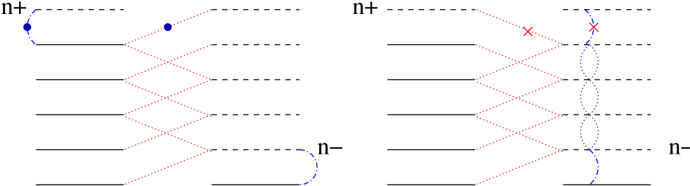
Figure 2: (Color online) Left panel shows possible interband (dotted line) and intraband (dash-dotted line) transitions of the model. The solid (dashed) line shows filled (empty) states. For convention the $\lambda=-1$ states are plotted lower. The right panel shows the equivalence of equations (15) and (14). Two subtracted $\times$ transitions and two added $\bullet$ transitions are  ‘surface‘ terms in (15).

For a given physical system the SO parameter $\gamma_{0}$ may depend on the intrinsic and applied electric fields.win2 The Fermi energy depends linearly on the hole density $n_{D}$. Moreover $\gamma\sqrt{n_{f}}=(2m)^{3/2}\gamma_{0}\sqrt{{\varepsilon}_{f}}$ is independent of the applied magnetic field. In the accumulation layer of $GaAs-Al_{0.5}Ga_{0.5}As$ one obtains $\gamma\sqrt{n_{f}}\approx 0.3$ for $n_{D}=10^{10}cm^{-2}$ while in a $200$Å-wide quantum well with $n_{D}=10^{11}cm^{-2}$ we get $\gamma\sqrt{n_{f}}\approx 10^{-3}$.win2

We study the SHC as function of this parameter. When plotted against this parameter all graphs of SHC for different Fermi energies (hole densities) will be scaled to one graph. To begin with, the value of $\gamma$ is limited by $1<\gamma n_{f}^{3/2}<n_{f}$ which corresponds to $\hbar/\tau_{c}<\gamma_{0}(2m{\varepsilon}_{f})^{3/2}<{\varepsilon}_{f}$, i.e the same conditions as in the free hole system in which the relaxation time $\tau$ is replaced by the cyclotron time $\tau_{c}=1/\omega_{c}$. For this value of $\gamma$ the mixing angle $\theta^{\lambda}$ approaches its maximum value $-\pi/4$ and the conductivity (14) can be approximated as:

$$\sigma^{z,s}_{xy}(0)\approx-9\frac{e}{2\pi\hbar}(1/\gamma\sqrt{n^{+}}-1/\gamma\sqrt{n^{-}}+1).$$ (17)

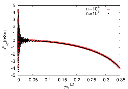
Figure 3: (Color online) The effective spin Hall conductivity as a function of $\gamma\sqrt{n_{f}}=\gamma_{0}\sqrt{{\varepsilon}_{f}}$ for different values of Fermi energy. All graphs scale to one if plotted against $\gamma\sqrt{n_{f}}$. For weak SO coupling or low Fermi energies the conductivity approaches zero but it shows Shubnikov-de Haas oscillations.

In Fig. 3 we have plotted the effective SHC (14) as a function of $\gamma\sqrt{n_{f}}$. For larger value of $\gamma\sqrt{n_{f}}$ the effective SHC $\sigma^{z,s}_{xy}$ is negative and finite. The negative sign of the effective SHC for larger $\gamma\sqrt{n_{f}}$ is the result of the original choice for positive conventional SHC.Rashba3

For lower values of $\gamma\sqrt{n_{f}}$ both the effective and conventional SHC approach zero. In Fig. 4 we have plotted the effective SHC for lower values of $\gamma\sqrt{n_{f}}$. Going to the zero limit the typical Shubnikov-de Haas oscillations appear in the conductivity. Notice that for smaller $n_{f}$ the amplitude of the oscillations is larger, as one would expect for the quantum limit.

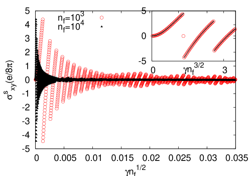
Figure 4: (Color online) The effective spin Hall conductivity for very low value of $\gamma\sqrt{n_{f}}\sim\gamma_{0}\sqrt{{\varepsilon}_{f}}$. The higher the $n_{f}$ values the smaller is the amplitude of oscillations, as one would expect. The inset is exactly the same graph when plotted against $\gamma{n_{f}}^{3/2}$ which shows that the highest jump in SHC is $\Delta\sigma^{s}_{xy}=9e/(8\pi)$ and it happens at the same value of $\gamma{n_{f}}^{3/2}$ for any $n_{f}$.

It is important to note that the same behavior can be observed for effective SHC in the linear Rashba model in a magnetic field. Actually the formula (14) is valid for $k$-linear Rashba model (up to the factor of 9 which comes from spin-3/2 holes and $k^{3}$ momentum dependence). In Fig. 5 we compare the effective SHC of these two models. There are two differences between the two systems. Firstly in the $k$-linear Rashba model with $V_{SO}=\alpha(k\times\sigma)$ the effective SHC remains zero for larger value of SO coupling $\alpha$ while in the $k$-cubic model it goes to finite negative values (see Fig. 3). However the deviation from zero in the latter case is because we approach the limit of unbounded negative energies while for the linear model the typical value of SO coupling is very far from the upper limit $\alpha>\sqrt{n_{f}}$ of the unphysical region. Second and more importantly, in the linear model both the interband and intraband contributions to the effective SHC are zero independently while for the $k$-cubic model these two contributions are finite but opposite in sign and cancel each other out.

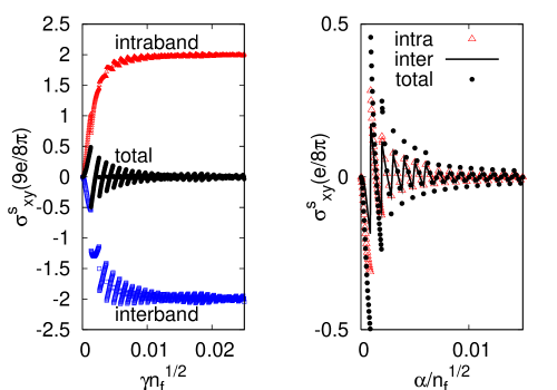
Figure 5: (Color online) The distinct intra and interband transition contributions to the effective SHC for very low value of $\gamma\sqrt{n_{f}}$ in the $k$-cubic model (left panel). The right panel is the same for the $k$-linear model in which two contributions are zero independently.

For comparison we also calculate the conventional SHC (12). A straightforward replacement of the wave functions and energies in (12) renders

$$\sigma^{z}_{xy}(0)=\frac{3e}{4\pi\hbar}\sum_{n,\lambda\lambda^{\prime}}^{*}$$

$$\frac{(n-1)\cos^{2}\theta_{n+1}^{\lambda^{\prime}}\cos^{2}\theta_{n}^{\lambda}-(n+2)\sin^{2}\theta_{n+1}^{\lambda^{\prime}}\sin^{2}\theta_{n}^{\lambda}}{1+\delta/\cos 2\theta_{n+1}^{\lambda^{\prime}}-\delta/\cos 2\theta_{n}^{\lambda}}$$

$$-\frac{(n-2)\cos^{2}\theta_{n-1}^{\lambda^{\prime}}\cos^{2}\theta_{n}^{\lambda}-(n+1)\sin^{2}\theta_{n-1}^{\lambda^{\prime}}\sin^{2}\theta_{n}^{\lambda}}{1+\delta/\cos 2\theta_{n}^{\lambda}-\delta/\cos 2\theta_{n-1}^{\lambda^{\prime}}}$$

(18)

in which the first (respectively second) term describes the transition $n\to n+1$ (respectively $n\to n-1$). We first include only the interband contribution to the conventional SHE to compare it to the system of free holes in the absence of magnetic field. The result is plotted in Fig. 6 and it is actually the same as the SHC for a free 2D electron gas.sch For the range of $\gamma\sqrt{n_{f}}$ chosen here, (18) can be approximated by

$$\sigma^{z,inter}_{xy}(0) \approx \frac{3e}{16\pi\hbar}\int_{n^{-}}^{n^{+}}\frac{-3}{\gamma\sqrt{n^{3}}}dn$$ (19)

$$= \frac{9e}{8\pi\hbar\gamma}(\frac{1}{\sqrt{n^{+}}}-\frac{1}{\sqrt{n^{-}}}).$$

which using $\hbar\omega_{c}n^{\pm}=\hbar^{2}k_{\pm}^{2}/2m$ renders exactly (4). Here, as $\gamma$ decreases the conventional SHC approaches its universal value $\sigma^{z}_{xy}=9e/8\pi$.sch Now we include also the intrabandr transitions, consisting of the two terms near the Fermi surface. Their contribution is negative and cancels the conventional SHC for the lower values of $\gamma\sqrt{n_{f}}$, as it is shown in the inset of Fig. 6

Figure 6: (Color online) The interband contribution to the conventional SHC as a function of $\gamma\sqrt{n_{f}}=\gamma_{0}\sqrt{{\varepsilon}_{f}}$ for the $k$-cubic model. For weak SO coupling or low Fermi energies the conductivity approaches its universal value $\sigma^{z}_{xy}=9e/8\pi$. When the intraband contribution is included, the total conventional SHC is zero for small $\gamma\sqrt{n_{f}}$ and goes to negative values as $\gamma\sqrt{n_{f}}$ increases.

V Conclusion

We have studied the 2D hole gas system with $k$-cubic Rashba SO interaction in a perpendicular magnetic field in the absence of Zeeman splitting. The exact eigenstates and eigenvalues are derived and used in a Kubo formula to calculate the effective and conventional SHC of the model. For the conventional SHC the interband transitions reproduce the intrinsic spin Hall conductivity which approaches the universal value of $\sigma^{z}_{xy}=9e/8\pi$ for weak SO coupling.sch However when the negative intraband contributions are included the conventional SHC becomes negative and goes to zero for weak SO coupling.

We also consider the effective spin current in which the torque dipole is included. We show that the corresponding effective SHC shows Shubnikov-de Haas oscillations around zero for small SO coupling, if both interband and intraband contributions are included. Higher $n_{f}$ results in smaller oscillation amplitude. For stronger SO coupling the effective SHC becomes negative.

Comparing the $k$-cubic model with the $k$-linear model, the main difference is that in the former the intraband and interband contributions to the effective SHC are finite but opposite in sign and cancel each other. In the latter each contribution is zero independently.

The fact that for low values of SO coupling both the effective and conventional SHC go to zero is unexpected. For the $k$-linear model it is well-known that the intraband transitions evolve into the vertex correction which is proved to be zero. For the $k$-cubic model, although it is well knownber ; lei ; mur that the vertex corrections are zero in the case of short-range s-wave scatterers, the relation between the intraband transitions and the vertex corrections is not straightforward. For the effective SHC eq.(16) suggests that the zero magnetic field limit is singular in this model. However more detailed calculations of the vertex and higher order corrections may help to ascertain this behavior.

The above results would be modified for an inhomogeneous system and for the ac SHC $\sigma^{z}_{xy}(\omega)$, because the intraband contributions are less stable and are reduced by frequency and scattering.mish One expects that the intraband contributions will diverge at $\omega=\omega_{c}$ after which they will vanish for $\omega_{c}\ll\omega$.

Acknowledgment

The work was supported by CMSS at Ohio University and NSF-NIRT.

References

- (1) A review on spin Hall transport is given in S. Murakami cond-mat/0504353. J. Sinova, S. Murakami, S.Q. Shen, M. S. Choi cond-mat/0512054 and J. Schliemann cond-mat/0602330.
- (2) M. I. D’yakonov and V. I. Perel’, ZhETF Pis. Red. 13, 6 57 (1971) [JETP Lett. 13, 467 (1971)]; J. E. Hirsch, Phys. Rev. Lett. 83, 1834 (1999); S. Zhang, Phys. Rev. Lett. 85, 393 (2000).
- (3) S. Murakami, N. Nagaosa, and S. C. Zhang, Science 301, 1348 (2003); S. Murakami and N. Nagaosa, Phys. Rev. Lett. 90, 057002 (2003).
- (4) J. M. Luttinger, Phys. Rev. 102, 1030 (1956).
- (5) J. Sinova, Dimitrie Culcer, Q. Niu, N. A. Sinitsyn, T. Jungwirth, and A. H. MacDonald, Phys. Rev. Lett. 92, 126603 (2004).
- (6) E. I. Rashba, Sov. Phys. Solid state 2, 1109 (1960).
- (7) Y. K. Kato, R. C. Myers, A. C. Gossard, D. D. Awschalom, Science, 306, 1910 (2004)
- (8) J. Wunderlich, B. Kaestner, J. Sinova, T. Jungwirth, Phys. Rev. Lett. 94 047204 (2005).
- (9) Hans-Andreas Engel, Bertrand I. Halperin, Emmanuel I. Rashba,cond-mat/0505535
- (10) B. A. Bernevig and S. C. Zhang, Phys. Rev. Lett. 95, 016801 (2005)
- (11) S. Y. Liu and X. L. Lei, Phys. Rev. B 72, 155314 (2005) and S. Y. Liu and X. L. Lei, Phys. Rev. B 72, 249901(E) (2005)
- (12) Shichi Murakami, Phys. Rev. B. 69, 241202(R) (2004).
- (13) J. I. Inoue, G. E. W. Bauer, and L. W. Molenkamp, Phys. Rev. B 67, 033104 (2003).
- (14) J. Inoue, G. E. W. Bauer, and L. W. Molenkamp, cond-mat/0402442.
- (15) O. V. Dimitrova, Phys. Rev. B 71, 245327 (2005).
- (16) O. Chalaev and D. Loss, Phys. Rev. B 71, 245318 (2005).
- (17) E.G. Mishchenko, A. V. Shytov and B. I. Halperin, Phys, Rev. Lett 93, 226602 (2004).
- (18) R. Raimondi and P. Schwab, PRB 71, 033311 (2005).
- (19) A.Khaetskii, cond-mat/0408136
- (20) K. Nomura, J. Sinova, N. A. Sinitsyn, and A. H. MacDonald , cond-mat/0506189.
- (21) L. Sheng, D. N. Sheng, and C. S. Ting, Phys. Rev. Lett.94, 016602 (2005).
- (22) Branislav K. Nikolic, S. Souma, Liviu P. Zarbo, and Jairo Sinova, Phys. Rev. Lett. 95, 046601 (2005)
- (23) R. Winkler, Phys. Rev. B 62, 4245 (2000); R. Winkler, H. Noh, E. Tutuc, and M. Shayegan, Phys. Rev. B 65, 155303 (2002)
- (24) In (1) we use the Hamiltonian of ref. win2 which is an invariant of group. In some of the literature the SO term is written as which is an invariant of group. We have got the same SHC for the latter model. We are grateful to E. I. Rashba for bringing this point to our attention.
- (25) J. Schliemann and D. Loss, Phys. Rev. B 71, 085308 (2005).
- (26) W. Q. Chen, Z. Y. Weng and D. N. Sheng, cond-mat/0502570 v3
- (27) S. Q. Shen, Phys. Rev. B 70, 081311(R) (2004). N. A. Sinitsyn, E. M. Hankiewicz, W. Teizer, J. Sinova, Phys. Rev. B 70, 081312(R) (2004).
- (28) E. I. Rashba, Phys. Rev. B 70, 201309(R) (2004).
- (29) E. I. Rashba, J. Supercond. 18, 137 (2005); E. I. Rashba, cond-mat/0507007.
- (30) E. I. Rashba, Phys. Rev. B 68, 241315(R) (2003).
- (31) G. Dresselhaus, Phys. Rev. B 100, 580 (1955).
- (32) M. Zarea and S. E. Ulloa Phys. Rev. B 72, 085342 (2005)
- (33) J. Schliemann, J. C. Egues, and D. Loss, Phys. Rev. B 67, 085302 (2003).
- (34) D. Culcer, J. Sinova, N. A. Sinitsyn, T. Jungwirth, A. H. MacDonald and Q. Niu, Phys. Rev. Lett. 93 046602 (2004)
- (35) In the presence of Zeeman coupling look at S. Q. Shen, M. Ma, X. C. Xie and F. C. Zhang, Phys. Rev. Lett. 92, 256603 (2004). S. Q. Shen,Y. J. Bao, M. Ma, X. C. Xie and F. C. Zhang, Phys. Rev. B 71, 155316 (2005).
- (36) R. Winkler, Spin-orbit coupling effects in two-dimensional electron and hole systems (Springer-Verlag, Berlin, 2003).
- (37) J. Shi, P. Zhang, D. Xiao and Q. Niu, Phys. Rev. Lett.96, 076604 (2006).
- (38) K. Nomura, J. Wunderlich, J. Sinova, B. Kaestner, A.H. MacDonald, T. Jungwirth, cond-mat/0508532
- (39) A. Khaetskii, cond-mat/0510815 v2
- (40) A. V. Shytov, E.G.Mishchenko, H.-A.Engel, B.I.Halperin , cond-mat/0509702 v2