Profiles of near-resonant population-imbalanced trapped Fermi gases

Abstract

We investigate the density profiles of a partially polarized trapped Fermi gas in the BCS-BEC crossover region using mean field theory within the local density approximation. Within this approximation the gas is phase separated into concentric shells. We describe how the structure of these shells depends upon the polarization and the interaction strength. A comparison with experiments yields insight into the possibility of a polarized superfluid phase.

I Introduction

Advances in the trapping and manipulating of degenerate Fermi atoms are attracting intense interest from physicists in the fields of condensed matter physics, atomic molecular and optical physics, nuclear physics, astrophysics, and particle physics. Current and future experiments aim to use this highly controlled environment to explore many-body phenomena with impact on widely varying areas of physics. We discuss the theory of one such set of phenomena; the properties of trapped partially polarized fermionic atoms, where the two spin states have different Fermi surfaces.

The study of Fermi systems with mismatched Fermi surfaces began with attempts by Fulde and Ferrell and Larkin and Ovchinnikov (FFLO)fflo to understand magnetized superconductors. More recent work has come from researchers in the nuclear physics community who are studying superconductivity in nuclear matter and quark matter, with a possible application to neutron stars or heavy ion collisions nm . Such calculations have taken on new relevance with the possibility of cold gas experiments where alkali atoms are trapped in a number of distinguishable hyperfine states, with negligible spin relaxation. Thus one can produce a two-component Fermi gas with arbitrary population imbalance. Using magnetic-field driven Feshbach resonances feshbach , the interactions between these atoms can be made large enough to drive the system superfluid.

Very recently, there have been two experimental studies of trapped ⁶Li Fermi atoms with mismatched Fermi surfaces ketterle ; randy . By analyzing time-of-flight images, Zwierlein et al. ketterle found evidence for phase separation between regions of equal and unequal population density. Furthermore, by studying vortices, they were able to monitor the evolution of superfluidity as a function of population imbalance: finding not only that polarization inhibits superfluidity, but that the superfluid region appears to coincide with the region of equal density. The equally exciting work of Partridge et al. randy directly shows phase separation through high resolution in-situ images of the atomic clouds.

In this paper, we study the density profile in the entire BCS-BEC crossover region within mean field theory. We use a local density approximation (LDA) and compare our results with experiments. Our study shows that the population imbalanced trapped Fermi gas is generically phase separated into concentric shells. Within our approximations, each region of space can be in one of several phases: unpolarized superfluid (S), polarized superfluid (PS), normal mixture (M), or fully polarized normal (P). The unpolarized superfluid coincides with the standard equal-population superfluid predicted by the BCS-BEC crossover theory crossover ; model1 ; model2 ; model3 ; cre . The polarized superfluid, which in mean-field theory is only found on the BEC side of resonance, consists of an interpenetrating gas of bosonic molecules and a fully polarized gas of fermions dan ; pao . The normal mixture and fully polarized normal phases both lack superfluidity and are distinguished by the presence or absence of the minority species of fermion. Due to the extremely small portion of the phase diagram where it is expected to appear, we do not consider the possibility of an inhomogeneous FFLO phase. As seen in a number of recent papers dan ; kinnunen ; castorina , such a phase would appear on the BCS side of resonance as a subtle structure in the domain wall separating the S and M regions.

Figure 1: Mean-field phase diagram of homogeneous two-component Fermi gas in the (a), (b) BEC and (c) BCS regimes. Phases only depend on the dimensionless ratio of the chemical potentials $\mu=(\mu_{\uparrow}+\mu_{\downarrow})/2$ and $h=(\mu_{\uparrow}-\mu_{\downarrow})/2$, and the energy scale of the interactions, $\epsilon=\hbar^{2}/2ma^{2}$. Panels (a) and (b) differ only by the scale used.

We find three different parameter regimes, distinguished by the structure of these shells: (1) BCS regime where $(k_{f}a)^{-1}\lesssim 0$, (2) crossover-BEC regime where $0\lesssim(k_{f}a)^{-1}\lesssim 1$, and (3) deep-BEC regime where $(k_{f}a)^{-1}\gtrsim 1$. The Fermi wave vector is $k_{f}$ and the scattering length is $a$. Depending upon density and polarization, regime (1) contains two scenarios – from center to edge one finds S-M-P or M-P. In regime (2) one finds S-P at small polarizations and S-M-P or M-P for larger. In regime (3) one finds S-PS-P for small polarizations and PS-P for larger polarizations note . In an appropriately defined thermodynamic limit there is a quantum phase transition between each of these possibilities as one varies the parameters of the system. This behavior should be contrasted with the smooth crossover physics found in the absence of a population imbalance.

Our results are consistent with the experiments reported in Ref. ketterle , however, due to the expansion procedure used in those experiments no quantitative comparison can be made. We find partial agreement with the experiments reported in Ref. randy . In particular, for sufficiently large polarizations we reproduce the values of the axial radius of the superfluid core and the outer edge of the gas cloud found in the experiments randy . Our total density profiles also closely agree with the experiments. However, we find that the spatial structure of the difference between up and down spins differs significantly from those found in the experiment randy . In particular, we show that despite the large ratio of the trap size to the coherence length, the experimental data are inconsistent with any LDA that assumes a harmonic trap, regardless of the equation of state used.

The most significant open theoretical question at the moment is the possibility of a polarized superfluid region at unitarity (UPS). As seen from the $\epsilon\rightarrow 0$ behavior of Fig. 1(b), the mean-field calculation predicts that such a region does not exist. Monte Carlo calculations suggest that such a region may exist, but are currently not conclusive carleson . Based upon a comparison with our mean-field calculations we argue that the experimental measure of phase separation (from analyzing the density profiles) is slightly ambiguous and one may be able to explain the experiments without recourse to a UPS. On the other hand, the poor agreement in the radii at small polarizations may support the notion of a UPS.

Concurrent with the preparation of this manuscript several authors kinnunen ; new presented complementary theoretical studies of the effect of trap potentials on a partially polarized gas. With the exception of Ref.dan , which discusses some qualitative feature of the trapped gas, prior theoretical work on superfluidity with mismatched Fermi surfaces has been restricted to either homogeneous systems homo ; breached ; dan ; pao ; paulo or trapped systems in the weakly coupling limit castorina .

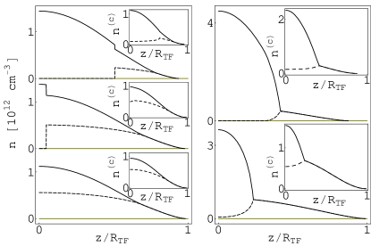
Figure 2: On-axis mean-field density profiles $n(z,\rho=0)$ of zero temperature harmonically trapped partially polarized Fermi gas, illustrating all of the cases described in the text. Solid lines show total density $n_{\uparrow}+n_{\downarrow}$, while dashed lines show density differences $n_{\uparrow}-n_{\downarrow}$. Left (right) figures represent the strong coupling BCS (BEC) regime with $k_{f}a=-2$, (0.5). The Thomas-Fermi radius is defined as $R_{TF}=\sqrt{(2\epsilon_{f})/(m\omega_{z}^{2})}$, where $\epsilon_{f}=\hbar^{2}k_{f}^{2}/2m=\hbar\overline{\omega}(6N)^{1/3}$ with average trap frequency $\overline{\omega}=(\omega_{\perp}^{2}\omega_{z})^{1/3}$. Inset shows column density $n^{(c)}=\int d\rho\,n(z,\rho)$ measured in units of [$10^{9}$ cm^-2]. All graphs use $N_{\uparrow}+N_{\downarrow}=2\times 10^{5}$ atoms in an axial symmetric trap with $\omega_{z}=2\pi\times 7.2Hz$, and $\omega_{\perp}=2\pi\times 350Hz$. BCS figures (top to bottom) have polarizations $P=(N_{\uparrow}-N_{\downarrow})/(N_{\uparrow}+N_{\downarrow})=0.30,0.74,0.80$ and BEC figures have $P=0.33,0.90$.

II Theory

We restrict ourselves to the wide resonance of ⁶Li where both of the available experiments ketterle ; randy have been carried out, and therefore we do not need to explicitly consider the closed channel of the Feshbach resonance. The fermions of different hyperfine states $\uparrow$ and $\downarrow$ interact through a short-range effective potential $-u\delta(\vec{r}\prime-\vec{r})$. The system of $N=N_{\uparrow}+N_{\downarrow}$ atoms is then described by the Hamiltonian model1 ; model2 ; model3 $H=H_{1}+H_{2}$, with $H_{1}=\sum_{\sigma}\int d^{3}\vec{r}\,\psi_{\sigma}^{\dagger}(\vec{r})[-\frac{\hbar^{2}\nabla^{2}}{2m}-\mu_{0\sigma}+V(\vec{r})]\psi_{\sigma}(\vec{r})$ containing kinetic and trapping energies and $H_{2}=-u\int d^{3}\vec{r}\psi^{\dagger}_{\uparrow}(\vec{r})\psi^{\dagger}_{\downarrow}(\vec{r})\psi_{\downarrow}(\vec{r})\psi_{\uparrow}(\vec{r})$ containing interactions. The field operators $\psi_{\sigma}(\vec{r})$ obey the usual fermionic anticommutation rules, and describe the annihilation of a fermion at position $\vec{r}$ in the hyperfine state $\sigma$. Parameters $m$, $\mu_{0\sigma}$ and $V(\vec{r})=\frac{1}{2}m(\omega_{\perp}^{2}\rho^{2}+\omega_{z}^{2}z^{2})$ are the mass, chemical potential, and trapping potential of the atomic species $\sigma$. We introduce a local chemical potential $\mu_{\sigma}(\vec{r})=\mu_{0\sigma}-V(\vec{r})$ and treat the system as locally homogeneous. Without loss of generality, we take $\uparrow$ to be the majority species of atoms and describe the system in terms of the spatially independent chemical potential difference $h=(\mu_{\uparrow}-\mu_{\downarrow})/2\geq 0$, and the spatially dependent average chemical potential $\mu(\vec{r})=(\mu_{\uparrow}+\mu_{\downarrow})/2$. Using the usual BCS mean-field decoupling, the BCS-Bogoliubov excitation spectrum of each species is given by $E_{k\sigma}(\vec{r})=\xi_{\sigma}h+\sqrt{(\epsilon_{k}-\mu)^{2}+\Delta^{2}}$. Here $\epsilon_{k}=\hbar^{2}k^{2}/2m$ is the kinetic energy, $\Delta(\vec{r})=u\langle\psi_{\downarrow}(\vec{r})\psi_{\uparrow}(\vec{r})\rangle$ is the local superfluid order parameter, and $\xi_{\uparrow}=-1$ and $\xi_{\downarrow}=+1$.

At zero temperature, the gap $\Delta(\vec{r})$ and the the number densities $n(\vec{r})=n_{\uparrow}(\vec{r})+n_{\downarrow}(\vec{r})$, $n_{d}(\vec{r})=n_{\uparrow}(\vec{r})-n_{\downarrow}(\vec{r})$ satisfy

$$\frac{-m}{2\pi\hbar^{2}a} = \int_{0}^{\infty}\frac{d^{3}\vec{k}}{(2\pi)^{3}}\left(\frac{1}{E_{k}}-\frac{1}{\epsilon_{k}}\right)-\int^{k_{+}}_{k_{-}}\frac{d^{3}\vec{k}}{(2\pi)^{3}}\frac{1}{E_{k}}$$ (1)

$$n(\vec{r}) = \int_{0}^{\infty}\frac{d^{3}\vec{k}}{(2\pi)^{3}}(1-\frac{\epsilon_{k}-\mu}{E_{k}})+\int^{k_{+}}_{k_{-}}(\frac{\epsilon_{k}-\mu}{E_{k}})$$ (2)

$$n_{d}(\vec{r}) = \frac{1}{(2\pi)^{3}}\frac{4\pi}{3}(k_{+}^{3}-k_{-}^{3}).$$ (3)

We define $E_{k}(\vec{r})=(E_{k\uparrow}+E_{k\downarrow})/2$, and $k_{\pm}(\vec{r})=(\pm\sqrt{h^{2}-\Delta^{2}}+\mu)^{1/2}$. The ultraviolet divergence associated with the delta-function interaction has been eliminated model1 ; model2 ; cre ; reg by introducing the effective scattering length through $-{m}/({4\pi\hbar^{2}a})={u}^{-1}-\int_{0}^{\infty}{d^{3}\vec{k}}{(2\pi)^{-3}}/{2\epsilon_{k}}.$ Notice that $n_{d}(\vec{r})$ is nonzero as long as $h>\Delta$ and $\mu>-\sqrt{h^{2}-\Delta^{2}}$.

At each point in space one finds $\Delta$ by solving Eq. (1) at fixed $\mu$ and $h$. As a nonlinear equation, there are multiple solutions – some of which correspond to energy minima, some to saddle points. For example, the Sarma state breached ; paulo ; sarma appears as a saddle point. We take the lowest energy solution, producing the phase diagram illustrated in Fig. 1. Within the cloud $h$ is uniform, while $\mu$ varies monotonically from the center to edge of the cloud. The configurations of local phases, as described in the Introduction, are found by following vertical lines in the figure. One determines $\mu_{0}$ and $h$ by imposing a constraint on the total number of particles $N=\int d^{3}\vec{r}\,n(\vec{r})$ and the polarization $P=(N_{\uparrow}-N_{\downarrow})/N$. Typical density profiles are shown in Fig. 2. Evolution of the radii of phase boundaries are shown in Fig. 3.

III Experiments

There are profound differences in the full three-dimensional density profile of the experimental cloud of Ref. randy and our predictions. These differences are best seen by looking at the axial density profile $n_{d}^{(a)}(z)=2\pi\,\int d\rho\,\rho\,n_{d}(z,\rho)$, found by integrating the densities over both transverse directions. As shown in Fig. 4, we find a monotonic axial profile, while at polarizations above $P\approx 0.1$, Partridge et al. experimentally see a non monotonic density difference, with a dip in the center and horns on the edges. Despite these horns, our calculation of the total axial density $n^{(a)}(z)=2\pi\,\int d\rho\,\rho\,n(z,\rho)$ agrees extremely well with the experimental data (Fig. 5).

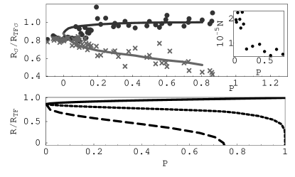
Figure 3: TOP: Radii of the minority and majority components using experimental parameters from Ref. randy . Dots and crosses are the experimental data for the majority and minority components respectively. Lines show our theoretical predictions with $k_{f}a=20.6$. The inset shows the total number of atoms used for calculation at each P. The two spin state radii $(R_{\uparrow},R_{\downarrow})$ are separately scaled by $R_{TF\uparrow}$ and $R_{TF\downarrow}$, where $R_{TF\sigma}$ is the Thomas-Fermi radius of a noninteracting one-component cloud with $N_{\sigma}$ atoms. BOTTOM: Radii of phase boundaries in the BCS regime with $k_{f}a=-2$. Solid, short-dashed, and long-dashed lines are the boundaries of polarized normal, normal mixture, and unpolarized superfluid, respectively. Input parameters are the same as those of figure 2, as is the definition of $R_{TF}$.

Assuming LDA in a harmonic trap, the density is only a function of $\mu(r)=\mu_{0}-m\omega_{\perp}^{2}\rho^{2}/2-m\omega_{z}^{2}z^{2}/2$. [As before, $\mu_{0}=(\mu_{0\uparrow}+\mu_{0\downarrow})/2$.] One can therefore write $n_{d}^{({a})}(z)=\frac{2\pi}{m\omega_{\perp}^{2}}f(\mu_{0}-m\omega_{z}^{2}z^{2}/2),$ where $f(\bar{\mu})=\int_{-\infty}^{\bar{\mu}}d\mu n_{d}(\mu).$ Since $n_{d}>0$ one has $f(\bar{\mu})$ is monotonic and $n_{d}^{({a})}(z)$ must decrease monotonically as $z$ increases from 0. In other words the horns seen in the experimental density differences are not consistent with the LDA. This result is based solely on the local density approximation and harmonic trapping – it does not require mean-field theory. We caution that this theorem only applies to the doubly integrated axial density, and not to the column density.

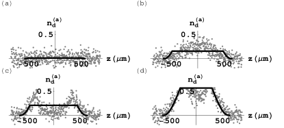
Figure 4: Doubly integrated axial density difference $n_{d}^{(a)}(z)=2\pi\,\int d\rho\,\rho\,[n_{\uparrow}(z,\rho)-n_{\downarrow}(z,\rho)]$ of zero temperature harmonically trapped partially polarized Fermi gas in units of $[10^{6}cm^{-1}]$. Figures (a), (b), (c), and (d) represent polarization $P=0.01$, 0.09, 0.14, and 0.53 respectively. All graphs use the experimental parameters from Ref. randy and the gray points are the experimental data.

Even if mean-field theory breaks down, these experiments should be well described by a local density approximation. The only relevant microscopic scale near unitary is the Fermi temperature $T_{f}\approx 400nK$, which is over 20 times larger than the quantization scale of the harmonic trap $\hbar\omega_{\perp}/k_{B}\approx 17nK$, which is a characteristic scale for density variations. We are currently investigating the possibility that surface tension in the domain wall between the polarized and superfluid regions may be distorting the shape of the boundary, leading to the observed density profiles.

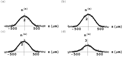
Figure 5: Comparison of the axial density $n^{(a)}(z)=2\pi\,\int d\rho\,\rho\,[n_{\uparrow}(z,\rho)+n_{\downarrow}(z,\rho)]$ in units of $[10^{6}cm^{-1}]$ with experimental data of Ref. randy . The labels are the same as those of Fig. 4.

Further experimental and theoretical work is needed to settle this issue. It is particularly important because Partridge et al. interpret the appearance of horns as a transition between a unitary polarized superfluid and a phase separation between superfluid and normal regions. Since the LDA predicts that the horns do not exist in a phase-separated cloud, we caution strongly against taking their disappearance as evidence for a polarized superfluid.

IV Acknowledgments

This work was supported by NSF grant No. PHY-0456261, and by the Alfred P. Sloan Foundation. We are grateful to R. Hulet and W. Li for very enlightening discussions, and for sending us the data in Figs. 3, 4, and 5. We thank D. E. Sheehy and L. Radzihovsky for the critical comments on the manuscript.

References

- (1) P. Fulde and R. A. Ferrell, Phys. Rev. 135, A550 (1964) and A.I. Larkin and Yu.N. Ovchinnikov, Zh. Eksp. Teor. Fiz 47, 1136 (1964) [Sov. Phys. JETP 20, 762 (1965)].
- (2) A. Sedrakian and U. Lombardo, Phys. Rev. Lett. 84, 602 (2000); J. A. Bowers and K. Rajagopal, Phys. Rev. D 66, 065002 (2002); I. Shovkovy and M. Huang, Phys. Lett. B 564, 205 (2003); R. Casalbuoni and G. Nardulli, Rev. Mod. Phys. 76, 263 (2004).
- (3) H. Feshbach, Ann.Phys. 19, 287 (1962).
- (4) Martin W. Zwierlein, Andr Schirotzek, Christian H. Schunck, Wolfgang Ketterle, Science, 311, 492 (2006).
- (5) Guthrie B. Partridge, Wenhui Li, Ramsey I. Kamar, Yean-an Liao, and Randall G. Hulet, Science, 311, 503 (2006).
- (6) A. J. Leggett, in Modern Trends in the Theory of Condensed Matter, edited by A. Pekalski and R. Przystawa (Springer-Verlag, Berlin, 1980); P. Nozieres and S. Schmitt-Rink, J. Low Temp. Phys. 59, 195 (1985); D. M. Eagles, Phys. Rev. 186, 456 (1969); A. Tokumitsu, K. Miyake and, K. Yamada, Phys. B 47, 11988 (1993); J. R. Engelbrecht, M. Randeria and C. A. R. Sa de Melo, Phys. Rev. B 55, 15153 (1997).
- (7) Y. Ohashi and A. Griffin, Phys. Rev. Lett. 89, 130402 (2002).
- (8) J. N. Milstein, S. J. J. M. F. Kokkelmans, and M. J. Holland, Phys. Rev. A 66, 043604 (2002).
- (9) E. Timmermans, K. Furuya, P. W. Milonni, and A. K. Kerman, Phys. Lett. A 285, 228 (2001); M. Holland, S. J. M. F. Kokkelmans, M. L. Chiofalo, and R. Walser, Phys. Rev. Lett. 87, 120406 (2001); A. Perali, P. Pieri, and, G. C. Strinati, Phys. Rev. A 68, 031601(R) (2003); T. Kostyrko and J. Ranninger, Phys. Rev. B 54, 13105 (1996).
- (10) C.A.R. S de Melo, M. Randeria, and J.R. Engelbrecht, Phys. Rev. Lett. 71, 3202 (1993); Y. Ohashi1 and A. Griffin, Phys. Rev. A 67, 033603 (2003); Y. Ohashi1 and A. Griffin, Phys. Rev. A 67, 063612 (2003).
- (11) D.E. Sheehy and L. Radzihovsky, PRL 96, 060401 (2006).
- (12) C.-H. Pao, Shin-TzaWu, and S.-K. Yip, preprint, cond-mat/0506437.
- (13) J. Kinnunen, L. M. Jensen, and P. Torma, Phys. Rev. Lett. 96, 110403 (2006).
- (14) P. Castorina, M. Grasso, M. Oertel, M. Urban, and D. Zappal‘a, Phys. Rev. A 72, 025601 (2005); T. Mizushima, K. Machida, and M. Ichioka, Phys. Rev. Lett. 94, 060404 (2005).
- (15) This PS-P shell structure was discussed in reference dan .
- (16) J. Carlson and S. Reddy, Phys. Rev. Lett. 95, 060401 (2005).
- (17) P. Pieri, and G.C. Strinati, PRL 96, 150404 (2006); W. Yi, and L. -M. Duan, Phys. Rev. A 73, 031604(R) (2006); F. Chevy, Phys. Rev. Lett. 96, 130401 (2006); H. Caldas, preprint, cond-mat/0601148; M. Haque and H.T.C. Stoof, preprint, cond-mat/0601321; Tin-Lun Ho and Hui Zhai, preprint cond-mat/0602568; Zheng-Cheng Gu, Geoff Warner and Fei Zhou, preprint cond-mat/0603091 ; M. Iskin and C. A. R. Sa de Melo, preprint cond-mat/0604184; T. Paananen, J.-P. Martikainen, P. Torma, preprint cond-mat/0603498.
- (18) R. Combescot, Europhys. Lett. 55, 150 (2001); H. Caldas, Phys. Rev. A 69, 063602 (2004); A. Sedrakian, J. Mur-Petit, A. Polls; H. M uther, Phys. Rev. A 72, 013613 (2005); U. Lombardo, P. Nozi‘eres, P. Schuck, H.-J. Schulze, and A. Sedrakian, Phys. Rev. C 64, 064314 (2001); D.T. Son and M.A. Stephanov, cond-mat/0507586; L. He, M. Jin and P. Zhuang, cond-mat/0601147.
- (19) W.V. Liu and F. Wilczek, Phys. Rev. Lett. 90, 047002 (2003).
- (20) P. F. Bedaque, H. Caldas, and G. Rupak, Phys. Rev. Lett. 91, 247002 (2003).
- (21) G. Sarma, J. Phys. Chem. Solids 24, 1029 (1963).
- (22) S.J.J.M.F. Kokkelmans, J.N. Milstein, M.L. Chiofalo, R. Walser, and M.J. Holland, Phys. Rev. A 65, 053617 (2002).