Bond-order modulated staggered flux phase for the $t{-}J$ model on the square lattice

Abstract

Motivated by the observation of inhomogeneous patterns in some high-T_c cuprate compounds, several variational Gutzwiller-projected wave-functions with built-in charge and bond order parameters are proposed for the extended $t-J-V$ model on the square lattice at low doping. First, following a recent Gutzwiller-projected mean-field approach by one of us (Phys. Rev. B. 72, 060508(R) (2005)), we investigate, as a function of doping and Coulomb repulsion, the stability of the staggered flux phase with respect to small spontaneous modulations of squared unit cells ranging from $2\times 2$ to $\sqrt{32}\times\sqrt{32}$. It is found that a $4\times 4$ bond-order (BO) modulation appears spontaneously on top of the staggered flux pattern for hole doping around $1/8$. A related wave-function is then constructed and optimized accurately and its properties studied extensively using an approximation-free variational Monte Carlo scheme. Finally, the competition of the BO-modulated staggered flux wave-function w.r.t. the d-wave RVB wave-function or the commensurate flux state is investigated. It is found that a short range Coulomb repulsion penalizes the d-wave superconductor and that a moderate Coulomb repulsion brings them very close in energy. Our results are discussed in connection to the STM observations in the under-doped regime of some cuprates.

I Introduction: models and methods

The observation of a d-wave superconducting gap in the high-$T_{c}$ cuprate superconductors suggests anderson_hgtc_hubbard that strong correlations are responsible for their unconventional properties and superconducting behavior. The two-dimensional (2D) $t{-}J$ model is one of the simplest effective models proposed Zhang-Rice to describe the low energy physics of these materials,

$$H_{t-J} = -t\sum\limits_{\langle i,j\rangle,\sigma}{\left(c_{i,\sigma}^{\dagger}c_{j,\sigma}+h.c.\right)}$$ (1)

$$+J\sum\limits_{\langle i,j\rangle}{\mathbf{S}_{i}\cdot\mathbf{S}_{j}}$$

The electrons are hopping between nearest neighbor sites of a square lattice leading to a kinetic energy term (first term of 1) as well as an exchange energy due to their spin interaction (second term), where $\mathbf{S}_{i}$ denotes the spin at site $i$: $\mathbf{S}_{i}=\frac{1}{2}c_{i,\alpha}^{\dagger}\vec{\sigma}_{\alpha,\beta}c_{i,\beta}$ and $\vec{\sigma}$ is the vector of Pauli matrices. $\langle i,j\rangle$ stands for a pair of nearest neighbors. $H_{t-J}$ operates only in the subspace where there are no doubly occupied sites, which can be formally implemented by a Gutzwiller projector (see later). In the following we set $\left|t\right|=1$ (unless specified otherwise) and we adopt a generic value of $t/J=3$ throughout the paper. Because of the particle-hole symmetry in the square lattice the sign of $t$ does not play any role. Although this model is formulated in a very simple form, the nature of the quantum correlations makes its physics very rich, and even the ground state of the $t{-}J$ hamiltonian was not yet characterized for finite doping and large cluster size. However, the $t{-}J$ model was investigated extensively by unbiased numerical techniques review_Dagotto as well as by mean-field kotliar_fluxphases and variational Monte-Carlo approaches yokoyama_mcv_supra ; gros_mcv_supra . All approaches found a d-wave superconducting phase and a phase diagram which accounts for most of the experimental features of the high-$T_{c}$ cupratesparamekanti_mcv ; RVB2 . In the limit of vanishing doping (half-filling), such a state can be viewed as an (insulating) resonating valence bond (RVB) or spin liquid state. In fact, such a state can also be written (after a simple gauge transformation) as a staggered flux state (SFP) kotliar_fluxphases ; half-flux , i.e. can be mapped to a problem of free fermions hopping on a square lattice thread by a staggered magnetic field.

Upon finite doping, although such a degeneracy breaks down, the SFP remains a competitive (non-superconducting) candidate with respect to the d-wave RVB superconductor staggered_flux . In fact, it was proposed by P.A. Lee and collaborators PLee1 ; PLee2 ; PLee3 that such a state bears many of the unconventional properties of the pseudo-gap normal phase of the cuprate superconductors. This simple mapping connecting a free fermion problem on a square lattice under magnetic field Hofstadter to a correlated wave-function (see later for details) also enabled to construct more exotic flux states (named as commensurate flux states) where the fictitious flux could be uniform and commensurate with the particle density Flux_phases_0 ; Flux_phases_1 . In this particular case, the unit-cell of the tight-binding problem is directly related to the rational value of the commensurate flux.

With an increasing number of materials and novel experimental techniques of constantly improving resolution, novel features in the global phase diagram of high-T_c cuprate superconductors have emerged. One of the most striking is the observation, in some systems, of a form of local electronic ordering, especially around $1/8$ hole doping. Indeed, recent scanning tunnelling microscopy/spectroscopy (STM/STS) experiments of underdoped Bi₂Sr₂CaCu₂O_8+δ (BSCO) in the pseudogap state have shown evidence of energy-independent real-space modulations of the low-energy density of states (DOS) STM-BSCO ; STM-BSCO-note ; STM_fourfold_structure ; STM_fourfold_charge_order with a spatial period close to four lattice spacings. A similar spatial variation of the electronic states has also been observed in the pseudogap phase of Ca_2-xNa_xCuO₂Cl₂ single crystals ($x=0.08\sim 0.12$) by similar STM/STS techniques STM2 . Although it is not clear yet whether such phenomena are either generic features or really happening in the bulk of the system, they nevertheless raise important theoretical questions about the stability of such structures in the framework of our microscopic strongly correlated models.

In this paper, we analyze the stability and the properties of new inhomogeneous phases (which may compete in certain conditions with the d-wave superconducting RVB state) by extending the previous mean-field and variational treatments of the RVB theory. In addition, we shall also consider an extension of the simple $t{-}J$ model, the $t-J-V$ model, containing a Coulomb repulsion term written as,

$$V=\frac{1}{2}\sum\limits_{i\neq j}V(|i-j|)\left(n_{i}-n\right)\left(n_{j}-n\right)\ ,$$ (2)

where $n$ is the electron density ($N_{e}/N$, $N_{e}$ electrons on a $N$-site cluster). Generically, we assume a screened Coulomb potential :

$$V(r)=V_{0}\frac{\exp^{-r/\ell_{0}}}{r}\ ,$$ (3)

where we will consider two typical values $\ell_{0}=2,4$ and $V_{0}\in[0,5]$ and where the distance $r$ is defined (to minimize finite size effects) as the periodized distance on the torus note_distance . The influence of this extra repulsive term in the competition between the d-wave RVB state and some inhomogeneous phases is quite subtle and will be discussed in the following.

To illustrate our future strategy, let us recall in more details the simple basis of the RVB theory. It is based on a mean-field hamiltonian which is of BCS type,

$$H_{\rm BCS}=\sum\limits_{\langle i,j\rangle,\sigma}\left(-\chi_{0}c_{i\sigma}^{\dagger}c_{j\sigma}+h.c.\right)\\ +\sum\limits_{\langle i,j\rangle}\left(\Delta_{i,j}c_{i\uparrow}^{\dagger}c_{j\downarrow}^{\dagger}+h.c.\right)-\mu\sum\limits_{i,\sigma}n_{i,\sigma}\ ,$$ (4)

where $\chi_{0}$ is a constant variational parameter and $\Delta_{i,j}$ is a nearest neighbor d-wave pairing (with opposite signs on the vertical and horizontal bonds) and $\mu$ is the chemical potential. As a matter of fact, the BCS mean-field hamiltonian can be obtained after a mean-field decoupling of the $t{-}J$ model, where the decoupled exchange energy leads to the $\chi_{0}$ and $\Delta_{i,j}$ order parameters. In this respect, we expect that the BCS wave-function is a good starting point to approximate the ground state of the $t{-}J$ model. However, such a wave-function obviously does not fulfill the constraint of no-doubly occupied site (as in the $t{-}J$ model). This can be easily achieved, at least at the formal level, by applying the full Gutzwiller operator Gutzwiller $\mathcal{P}_{\mathcal{G}}=\prod_{i}(1-n_{i\uparrow}n_{i\downarrow})$ to the BCS wave-function $\left|{\psi_{\rm BCS}}\right\rangle$:

$$\left|\psi_{\rm RVB}\right\rangle=\mathcal{P}_{\mathcal{G}}\left|{\psi_{\rm BCS}}\right\rangle\ .$$ (5)

The main difficulty to deal with projected wave-functions is to treat correctly the Gutzwiller projection $\mathcal{P}_{\mathcal{G}}$. This can be done numerically using a conceptually exact variational Monte Carlo (VMC) technique yokoyama_mcv_supra ; gros_mcv_supra ; paramekanti_mcv on large clusters. It has been shown that the magnetic energy of the variational RVB state at half-filling is very close to the best exact estimate for the Heisenberg model. Such a scheme also provides, at finite doping, a semi-quantitative understanding of the phase diagram of the cuprate superconductors and of their experimental properties. Novel results using a VMC technique associated to inhomogeneous wave-functions will be presented in Section III.

Another route to deal with the Gutzwiller projection is to use a renormalized mean-field (MF) theory Renormalized_MF in which the kinetic and superexchange energies are renormalized by different doping-dependent factors $g_{t}$ and $g_{J}$ respectively. Further mean-field treatments of the interaction term can then be accomplished in the particle-particle (superconducting) channel. Crucial, now well established, experimental observations such as the existence of a pseudo-gap and nodal quasi-particles and the large renormalization of the Drude weight are remarkably well explained by this early MF RVB theory RVB2 . An extension of this approach Renormalized_MF_2 ; Renormalized_MF_3 will be followed in Section II to investigate inhomogeneous structures with checkerboard patterns involving a decoupling in the particle-hole channel. As (re-) emphasized recently by Anderson and coworkers RVB2 , this general procedure, via the effective MF Hamiltonian, leads to a Slater determinant $\left|\Psi_{\rm MF}\right\rangle$ from which a correlated wave-function $\mathcal{P}_{\mathcal{G}}\left|\Psi_{\rm MF}\right\rangle$ can be constructed and investigated by VMC. Since the MF approach offers a reliable guide to construct translational symmetry-breaking projected variational wave-functions, we will present first the MF approach in section II before the more involved VMC calculations in Section III.

II Gutzwiller-projected mean-field theory

II.1 Gutzwiller approximation and mean-field equations

We start first with the simplest approach where the action of the Gutzwiller projector $\mathcal{P}_{\mathcal{G}}$ is approximately taken care of using a Gutzwiller approximation scheme Gutzwiller . We generalize the MF approach of Ref. Renormalized_MF_2, , to allow for non-uniform site and bond densities. Recently, such a procedure was followed in Ref. Renormalized_MF_3, to determine under which conditions a $4\times 4$ superstructure might be stable for hole doping close to $1/8$. We extend this investigation to arbitrary small doping and other kinds of supercells. In particular, we shall also consider 45-degree tilted supercells such as $\sqrt{2}\times\sqrt{2}$, $\sqrt{8}\times\sqrt{8}$ and $\sqrt{32}\times\sqrt{32}$.

The weakly doped antiferromagnet is described here by the renormalized $t{-}J$ model Hamiltonian,

$$H_{t-J}^{\rm ren}=-tg_{t}\sum_{\langle ij\rangle\sigma}(c^{\dagger}_{i,\sigma}c_{j,\sigma}+h.c.)+Jg_{J}\sum_{\langle ij\rangle}\mathbf{S}_{i}\cdot\mathbf{S}_{j}$$ (6)

where the local constraints of no doubly occupied sites are replaced by statistical Gutzwiller weights $g_{t}=2x/(1+x)$ and $g_{J}=4/(1+x)^{2}$, where $x$ is the hole doping. A typical value of $t/J=3$ is assumed hereafter.

Decoupling in both particle-hole and (singlet) particle-particle channels can be considered simultaneously leading to the following MF hamiltonian,

$$H_{\rm MF}=-t\sum_{\langle ij\rangle\sigma}g_{ij}^{t}(c^{\dagger}_{i,\sigma}c_{j,\sigma}+h.c.)+\sum_{i\sigma}\epsilon_{i}n_{i,\sigma}$$

$$-\frac{3}{4}J\sum_{\langle ij\rangle\sigma}g_{i,j}^{J}(\chi_{ji}c^{\dagger}_{i,\sigma}c_{j,\sigma}+h.c.-|\chi_{ij}|^{2})$$ (7)

$$-\frac{3}{4}J\sum_{\langle ij\rangle\sigma}g_{i,j}^{J}(\Delta_{ji}c^{\dagger}_{i,\sigma}c^{\dagger}_{j,-\sigma}+h.c.-|\Delta_{ij}|^{2}),$$

where the previous Gutzwiller weights have been expressed in terms of local fugacities $z_{i}=2x_{i}/(1+x_{i})$ ($x_{i}$ is the local hole density $1-\langle n_{i}\rangle$), $g_{i,j}^{t}=\sqrt{z_{i}z_{j}}$ and $g_{i,j}^{J}=(2-z_{i})(2-z_{j})$, to allow for small non-uniform charge modulations Anderson_suggestion_4a . The Bogoliubov-de Gennes self-consistency conditions are implemented as $\chi_{ji}=\langle c^{\dagger}_{j,\sigma}c_{i,\sigma}\rangle$ and $\Delta_{ji}=\langle c_{j,-\sigma}c_{i,\sigma}\rangle=\langle c_{i,-\sigma}c_{j,\sigma}\rangle$.

In principle, this MF treatment allows a description of modulated phases with coexisting superconducting order, namely supersolid phases. Previous investigations Renormalized_MF_3 failed to stabilize such phases in the case of the pure 2D square lattice (i.e. defect-free). Moreover, in this Section, we will restrict ourselves to $\Delta_{ij}=0$. The case where both $\Delta_{ij}$ and $\chi_{ij}$ are non-zero is left for a future work, where the effect of a defect, such as for instance a vortex, will be studied.

In the case of finite $V_{0}$ , the on-site terms $\epsilon_{i}$ may vary spatially as $-\mu+e_{i}$, where $\mu$ is the chemical potential and $e_{i}$ are on-site energies which are self-consistently given by,

$$e_{i}=\sum_{j\neq i}V_{i,j}\big{<}n_{j}\big{>}\,.$$ (8)

In that case, a constant $\sum_{i\neq j}V_{i,j}(\langle n_{i}\rangle\langle n_{j}\rangle+n^{2})$ has to be added to the MF energy. Note that we assume here a fixed chemical potential $\mu$. In a recent work chemical_function , additional degrees of freedom where assumed (for $V_{0}=0$) implementing an unconstrained minimization with respect to the on-site fugacities. However, we believe that the energy gain is too small to be really conclusive (certainly below the accuracy one can expect from such a simple MF approach). We argue that we can safely neglect the spatial variation of $\mu$ in first approximation, and this will be confirmed by the more accurate VMC calculations in Section III. Incidently, Ref. chemical_function, emphasizes a deep connection between the stability of checkerboard structures Renormalized_MF_3 and the instability of the SFP due to nesting properties of some parts of its Fermi surface susceptibility .

II.2 Mean-field phase diagrams

In principle, the mean-field equations could be solved in real space on large clusters allowing for arbitrary modulations of the self-consistent parameters. In practice, such a procedure is not feasible since the number of degrees of freedom involved is too large. We therefore follow a different strategy. First, we assume fixed (square shaped) supercells and a given symmetry within the super-cell (typically invariance under 90-degrees rotations) to reduce substantially the number of parameters to optimize. Incidently, the assumed periodicity allows us to conveniently rewrite the meanfield equations in Fourier space using a reduced Brillouin zone with a very small mesh. In this way, we can converge to either an absolute or a local minimum. Therefore, in a second step, the MF energies of the various solutions are compared in order to draw an overall phase diagram.

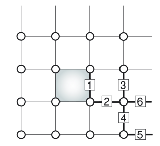
Figure 1: $4\times 4$ unit-cell used in both the MF approach and the variational wave-function. Note the existence of 6 independent bonds (bold bonds), that for convenience are labelled from $1-6$, and of 3 a priori non-equivalent sites. The center of the dashed plaquette is the center of the (assumed) $C_{4V}$ symmetry. Other sizes of the same type of structure are considered in the MF case, respectively : $2\times 2$, $\sqrt{8}\times\sqrt{8}$, and $\sqrt{32}\times\sqrt{32}$ unit cells.

In previous MF calculations Renormalized_MF_3 , stability of an inhomogeneous solution with the $4\times 4$ unit-cell shown in Fig. 1 was found around $x=1/8$. Here, we investigate its stability for arbitrary doping and extend the calculation to another possible competing solution with a twice-larger (square) unit-cell containing 32 sites. The general solutions with different phases and/or amplitudes on the independent links will be refered to as bond-order (BO) phases note_charge . Motivated by experiments STM-BSCO ; STM2 , a $C_{4V}$ symmetry of the inhomogeneous patterns around a central plaquette will again be assumed for both cases. Note that such a feature greatly reduces the number of variational parameters and hence speeds up the convergence of the MF equations. Starting from a central plaquette, like in Fig. 1, a larger $\sqrt{32}\times\sqrt{32}$ unit-cell (not shown) can easily be constructed with 10 non-equivalent bonds (with both independent real and imaginary parts) and a priori 6 non-equivalent sites. Note that this new unit-cell is now tilted by 45 degrees.

At this point, it is important to realize that patterns with a smaller number of non-equivalent bonds or sites are in fact subsets of the more general modulated structures described above. For example, the SFP is obviously a special case of such patterns, where all the $\chi_{i,j}$ are equal in magnitude with a phase oriented to form staggered currents, and where all the sites are equivalent. This example clearly indicates that the actual structure obtained after full convergence of the MF equations could have higher symmetry than the one postulated in the initial configuration which assumes a random choice for all independent parameters. In particular, the equilibrium unit-cell could be smaller than the original one and contain a fraction ($1/2$ or $1/4$) of it. This fact is illustrated in Fig. 2 showing two phase diagrams produced by using different initial conditions, namely $4\times 4$ (top) and $\sqrt{32}\times\sqrt{32}$ (bottom) unit-cells. Both diagrams show consistently the emergence of the SFP at dopings around $6\%$ and a plaquette phase ($2\times 2$ unit-cell with two types of bonds) at very small doping note_AF ; Vojta . In addition, a phase with a $\sqrt{8}\times\sqrt{8}$ super-cell is obtained for a specific range of doping and $V_{0}$ (see Fig. 2 on the top). Interestingly enough, all these BO phases can be seen as bond-modulated SFP with 2, 4, 8 and up to 16 non-equivalent (staggered) plaquettes of slightly different amplitudes. This would be consistent with the SFP instability scenario susceptibility which suggests that the wavevector of the modulation should vary continuously with the doping. Although this picture might hold when $V_{0}=0$, our results show that the system prefers some peculiar spatial periodicities (like the ones investigated here) that definitely take place at moderate $V_{0}$.

Figure 2: Mean-field phase diagrams obtained by solving self-consistently the mean-field equations on a $128\times 128$ lattice (for $\ell_{0}=4$) vs hole doping $x$ and repulsion $V_{0}$ (in units of $J$). Top: results obtained assuming a $4\times 4$ unit cell; Bottom: same with a $\sqrt{32}\times\sqrt{32}$ tilted unit cell. In both cases, a $C_{4v}$ symmetry is assumed (see text).

Let us now compare the two phase diagrams. We find that, except in some doping regions, the various solutions obtained with the $4\times 4$ unit-cell are recovered starting from a twice larger unit-cell. Note that, due to the larger number of parameters, the minimization procedure starting from a larger unit-cell explores a larger phase space and it is expected to be more likely to converge to the absolute minimum. This is particularly clear (although not always realized) at large doping $x=0.14$, where we expect an homogeneous Fermi Liquid (FL) phase (all bonds are real and equal), as indeed seen in Fig. 2 on the bottom. On the contrary, Fig. 2 on the top reveals, for $V_{0}/J\in[1.5,3]$, a modulated $\sqrt{8}\times\sqrt{8}$ structure, which is an artefact due to the presence of a local minimum (see next).

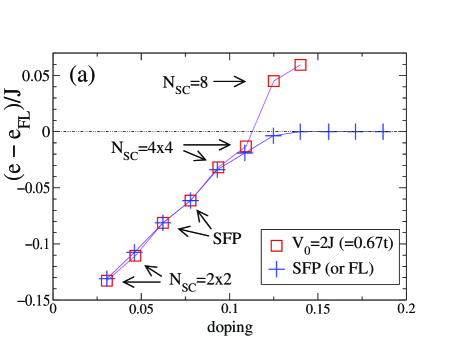
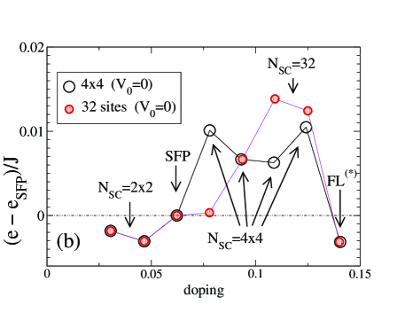
Figure 3: (Color online) (a) Energy per site (in units of $J$ and for $t=3J$) obtained by solving the mean-field equations using the initial $4\times 4$ unit-cell (see text) for a moderate value of $V_{0}$. The SFP energy is also shown for comparison. The FL energy has been substracted from all data for clarity. (b) Comparison of the energies (for $V_{0}=0$) using different initial conditions (see text), a $4\times 4$ or a $\sqrt{32}\times\sqrt{32}$ unit-cell; due to very small energy differences, the SFP energy is used as a reference for an easier comparison. The different phases specified by arrows and characterized by the number of sites $N_{SC}$ of their actual supercells refer to the ones in Fig. 2. For doping $x=0.14$, the minimization leads to a solution with small imaginary parts (of order $10^{-4}$) very similar to a FL phase, which we call FL^∗.

Since the MF procedure could accidentally give rise to local minima, it is of interest to compare the MF energies obtained by starting with random values of all independent parameters within the two previously discussed unit-cells. For convenience, we have substracted from all data either the FL (in Fig. 3(a)) or the SFP (in Fig. 3(b)) reference energy. From Figs. 3(a,b) we see that we can converge towards a local energy minimum, often modulated in space, which is not the absolute minimum. Indeed, over a large doping range, the lowest energy of the all solutions we have found is obtained for homogeneous densities and bond magnitudes. Nevertheless, we see that the $4\times 4$ modulated phase is (i) locally stable and (ii) is very close in energy to the homogeneous (SFP) phase which, often, has a slightly lower energy. Note that, around $x\simeq 1/8$, the states with $\sqrt{8}\times\sqrt{8}$ and $\sqrt{32}\times\sqrt{32}$ supercells are clearly metastable solutions (and using a larger initial unit-cell is not favorable in the latter case). In contrast, in this range of doping, the $4\times 4$ checkerboard state is very competitive w.r.t. the SFP. Therefore, it makes it a strong candidate to be realized either in the true ground state of the model, or present as very low excited state Vojta2 . In fact, considering such small energy differences, it is clear that an accurate comparison is beyond the accuracy of the MF approach. We therefore move to the approximation-free way of implementing the Gutzwiller projection with the VMC technique, that allows a detailed comparison between these variational homogeneous and inhomogeneous states.

III Variational Monte Carlo simulations of $4\times 4$ superstructures

Motivated by the previous mean-field results we have carried out extensive Variational Monte Carlo simulations. In this approach, the action of the Gutzwiller projection operator is taken care of exactly, although one has to deal with finite clusters. In order to get rid of discontinuities in the d-wave RVB wave-function, we consider (anti-)periodic boundary conditions along $e_{y}$ ($e_{x}$). As a matter of fact, it is also found that the energy is lower for twisted boundary conditions, hence confirming the relevance of this choice of boundaries. We have considered a $16\times 16$ square cluster of $N=256$ sites. We also focus on the $1/8$ doping case which corresponds here to $N_{e}=224$ electrons on the 256 site cluster. Following the previous MF approach, we consider the same generic mean-field hamiltonian,

$$H_{\rm MF}=\sum\limits_{\langle i,j\rangle,\sigma}\left(-\ {\tilde{t}}_{i,j}c_{i\sigma}^{\dagger}c_{j\sigma}+h.c.\right)+\sum\limits_{i\sigma}\epsilon_{i}c_{i\sigma}^{\dagger}c_{i\sigma}\,,$$ (9)

where the complex bond amplitudes ${\tilde{t}}_{i,j}$ can be written as $\left|{\tilde{t}}_{i,j}\right|e^{i{\theta}_{i,j}}$, and ${\theta}_{i,j}$ is a phase oriented on the bond $i\to j$. The on-site terms $\epsilon_{i}$ allow to control the magnitude of the charge density wave. However, the energy was found to be minimized for all the $\epsilon_{i}$ equal to the same value in the range $V_{0}=[0,5]$ and for the two parameters $\ell_{0}=2,4$. In fact, we find that strong charge ordered wave-functions are not stabilized in this model note_charge .

In this Section, we shall restrict ourselves to the $4\times 4$ unit-cell where all independent variational parameters are to be determined from an energy minimization. This is motivated both by experiments STM-BSCO ; STM2 and by the previous MF results showing the particular stability of such a structure (see also Ref. Renormalized_MF_3, ). As mentioned in the previous Section, we also impose that the phases and amplitudes respect the $C_{4V}$ symmetry within the unit-cell (with respect to the center of the middle plaquette, see Fig. 1), reducing the numbers of independent links to $6$. To avoid spurious degeneracies of the MF wave-functions related to multiple choices of the filling of the discrete k-vectors in the Brillouin Zone (at the Fermi surface), we add very small random phases and amplitudes ($10^{-6}$) on all the links in the $4\times 4$ unit cell.

Let us note that commensurate flux phase (CFP) are also candidate for this special $1/8$ doping. In a previous study, a subtle choice of the phases ${\theta}_{i,j}$ (corresponding to a gauge choice in the corresponding Hofstadter problem Hofstadter ) was proposed Flux_phases_1 , which allows to write the ${\phi}=p/16~{}(p<16)$ flux per plaquette wave-function within the same proposed unit-cell Flux_phases_1 and is also expected to lead to a better kinetic energy than the Landau gauge (in the Landau gauge the unit-cell would be a line of $16$ sites). However, we have found that the CFP wave-functions turned out not to be competitive for our set of parameters $V_{0}$, due to their quite poor kinetic energy, although they have very good Coulomb and exchange energies. We argue that such CFP wave-functions would become relevant in the large Coulomb and/or $J$ regimes (see table 1).

In order to further improve the energy, we also add a nearest-neighbor spin-independent Jastrow Jastrow_factor term to the wave-function,

$$\mathcal{P}_{\mathcal{J}}=\exp{\left(\alpha\sum\limits_{\langle i,j\rangle}{n_{i}n_{j}}\right)},$$ (10)

where $\alpha$ is an additional variational parameter. Finally, since the $t-J$ model allows at most one fermion per site, we discard all configurations with doubly occupied sites by applying the complete Gutzwiller projector $\mathcal{P}_{\mathcal{G}}$. The wave-function we use as an input to our variational study is therefore given by,

$$\left|\psi_{\rm var}\right\rangle=\mathcal{P}_{\mathcal{G}}\mathcal{P}_{\mathcal{J}}\left|{\psi_{\rm MF}}\right\rangle$$ (11)

In the following, we shall introduce simple notations for denoting the various variational wave-functions, $BO$ for the bond-order wave function, $SFP$ for the staggered flux phase, $RVB$ for the d-wave RVB superconducting phase, $FS$ for the simple projected Fermi-Sea, and we will use the notation $MF/\mathcal{J}$ ($MF=BO,SFP,RVB,FS$) when the Jastrow factor is applied on the mean-field wave-function. Finally, it is also convenient to compare the energy of the different wave-functions with respect to the energy of the simple projected Fermi-Sea (i.e. the correlated wave-function corresponding to the previous FL mean-field phase), therefore we define a condensation energy as $e_{c}=e_{var}-e_{FS}$.

Table 1: Set of energies per lattice site for $V_{0}=1$ and $\ell_{0}=4$ for different wave-functions. The best commensurate flux phase in the Landau gauge with flux per plaquette $p/16$ was found for $p=7$. We also show the energy of the CFP with flux $7/16$ written with another choice of gauge. We show the total energy per site ($E_{\rm{tot}}$), the kinetic energy per site ($E_{\rm{T}}$), the exchange energy per site ($E_{\rm{J}}$) and the Coulomb energy per site ($E_{\rm{V}}$).

wave-function	$E_{\rm{tot}}$	$E_{\rm{T}}$	$E_{\rm{J}}$	$E_{\rm{V}}$
$FS$	-0.4486(1)	-0.3193(1)	-0.1149(1)	-0.0144(1)
$CFP~{}7/16^{1}$	-0.3500(1)	-0.1856(1)	-0.1429(1)	-0.0216(1)
$CFP~{}7/16^{2}$	-0.4007(1)	-0.2369(1)	-0.1430(1)	-0.0208(1)
$SFP$	-0.4581(1)	-0.3106(1)	-0.1320(1)	-0.0155(1)
$BO$	-0.4490(1)	-0.3047(1)	-0.1302(1)	-0.0141(1)
$RVB$	-0.4564(1)	-0.3080(1)	-0.1439(1)	-0.0043(1)
$SFP/\mathcal{J}$	-0.4601(1)	-0.3116(1)	-0.1315(1)	-0.0169(1)
$BO/\mathcal{J}$	-0.4608(1)	-0.3096(1)	-0.1334(1)	-0.0177(1)
$RVB/\mathcal{J}$	-0.4644(1)	-0.3107(1)	-0.1440(1)	-0.0086(1)

¹ Landau gauge ² Gauge of Ref.Flux_phases_1,

Table 2: Order parameters for the different wave-functions for $V_{0}=1.5$ and $\ell_{0}=4$. We depict the following order parameters: $t_{i,j}\times e^{i\phi_{i,j}}$, where $t_{i,j}$ ($\phi_{i,j}$) is the amplitude (phase) of $\langle c_{i}^{+}c_{j}\rangle$, and the exchange energy $\langle S_{i}.S_{j}\rangle$, for the 6 independent bonds labelled for convenience according to Fig. 1. The sign of $\phi_{i,j}$ is according to the staggered flux pattern (see arrows in Fig. 9). We note that the $RVB/\mathcal{J}$ is uniform by construction. The variational superconducting order parameter is $\Delta_{RVB}=0.3$ for the $RVB/\mathcal{J}$ wave-function and $\Delta_{RVB}=0$ for the $SFP/\mathcal{J}$ and $BO/\mathcal{J}$ wave-functions.

	bond 1	bond 2	bond 3	bond 4	bond 5	bond 6
$t_{i,j}$
$RVB/\mathcal{J}$	0.077(1)	0.077(1)	0.077(1)	0.077(1)	0.077(1)	0.077(1)
$SFP/\mathcal{J}$	0.085(1)	0.085(1)	0.085(1)	0.085(1)	0.085(1)	0.085(1)
$BO/\mathcal{J}$	0.082(1)	0.083(1)	0.093(1)	0.088(1)	0.086(1)	0.084(1)
$\left|\phi_{i,j}\right|$
$RVB/\mathcal{J}$	0	0	0	0	0	0
$SFP/\mathcal{J}$	0.438(1)	0.438(1)	0.438(1)	0.438(1)	0.438(1)	0.438(1)
$BO/\mathcal{J}$	0.527(1)	0.502(1)	0.473(1)	0.390(1)	0.338(1)	0.384(1)
$-\langle S_{i}.S_{j}\rangle$
$RVB/\mathcal{J}$	0.215(1)	0.215(1)	0.215(1)	0.215(1)	0.215(1)	0.215(1)
$SFP/\mathcal{J}$	0.197(1)	0.197(1)	0.197(1)	0.197(1)	0.197(1)	0.197(1)
$BO/\mathcal{J}$	0.215(1)	0.207(1)	0.215(1)	0.187(1)	0.186(1)	0.170(1)

Figure 4: Energy per lattice site of the $RVB/\mathcal{J}$, $SFP/\mathcal{J}$ and $BO/\mathcal{J}$ wave-functions minus the energy of the projected Fermi-Sea wave-function.

In Fig. 4 we present the energies of the three wave-functions $BO/\mathcal{J}$, $SFP/\mathcal{J}$ and $RVB/\mathcal{J}$ for Coulomb potential $V_{0}\in[0,5]$. We find that for both $\ell_{0}=2$ and $\ell_{0}=4$ the $RVB$ phase is not the best variational wave-function when the Coulomb repulsion is strong. The bond-order wave-function has a lower energy for $V_{0}>2$ and $\ell_{0}=2$ ($V_{0}>1.5$ and $\ell_{0}=4)$. Note that the (short range) Coulomb repulsion in the cuprates is expected to be comparable to the Hubbard $U$, and therefore $V_{0}\approx 5$ or $10$ seems realistic. Independently of the relative stability of both wave-functions, the superconducting d-wave wave-function itself is strongly destabilized by the Coulomb repulsion as indicated by the decrease of the variational gap parameter for increasing $V_{0}$ and the suppression of superconductivity at $V_{0}\simeq 7$ (see Fig. 5).

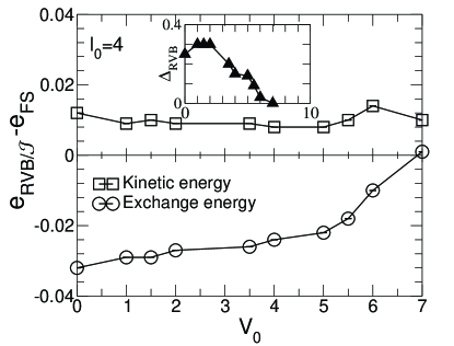
Figure 5: Kinetic and exchange energy per site of the $RVB/\mathcal{J}$ wave-function minus the respective exchange and kinetic energy of the simple projected Fermi-Sea. Inset: value of the variational d-wave gap.

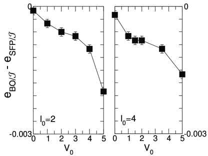
Figure 6: Total energy per site of the $BO/\mathcal{J}$ minus the energy of the $SFP/\mathcal{J}$ wave-functions.

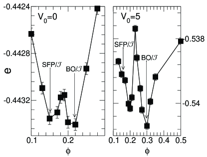
Figure 7: Total energy per site of the $BO/\mathcal{J}$ variational wave-function with variational parameters $Im\left({\tilde{t}}_{i,j}\right)=\pm\phi$ on the bonds $1,2,3$, and $Im\left({\tilde{t}}_{i,j}\right)=\pm 0.149$ on the bonds $4,5,6$. The sign of $Im\left({\tilde{t}}_{i,j}\right)$ is oriented according to the staggered flux pattern. We have chosen for all the links $Re\left(\ {\tilde{t}}_{i,j}\right)=0.988$. Results for $V_{0}=0$ and $V_{0}=5$ with $\ell_{0}=4$ are shown.

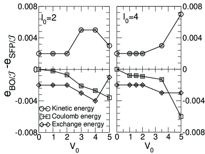
Figure 8: Kinetic, exchange and Coulomb energy per site of the $BO/\mathcal{J}$ wave-function minus the respective associated energy of the $SFP/\mathcal{J}$ wave-function.

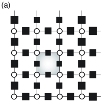
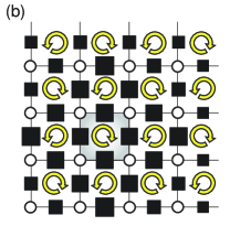
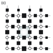
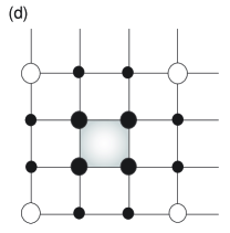
Figure 9: (Color online) Local expectation values (a,b,c) of the kinetic and exchange energies of the projected $BO/\mathcal{J}$ wave-functions on each of the bonds within the unit-cell. Width of filled square symbols is proportional to the (a) real and (b) imaginary part of $\langle c_{i}^{+}c_{j}\rangle$, and (c) to the local exchange energy $\langle\mathbf{S}_{i}\cdot\mathbf{S}_{j}\rangle$. The sign of the imaginary part of the hopping bonds is according to the staggered flux pattern (arrows). The wave-function has small charge density variations (d), therefore we subtract the mean value $n$ to the local density: size of circles are proportional to $\langle n_{i}-n\rangle$, and circles are open (filled) for negative (positive) sign. The biggest circle corresponds to an on-site charge deviation of $2\%$. All the above results are for $\l_{0}=4$ and $V_{0}=5$.

Nevertheless, we observe that the difference in energy between the bond-order wave-function and the staggered flux phase remains very small. We show in table 2 the order parameters measured after the projection for the $RVB/\mathcal{J}$, $SFP/\mathcal{J}$ and $BO/\mathcal{J}$ wave-functions. As expected the $RVB/\mathcal{J}$ and the $SFP/\mathcal{J}$ wave-functions are homogenous within the unit-cell. In contrast, the $BO/\mathcal{J}$ wave-function shows significant modulations (expected to be measurable experimentally) of the various bond variables w.r.t their values in the homogeneous SFP. In Fig. 6 we show the small energy difference (see scale) between the two wave-functions. Interestingly, the difference is increasing with the strength of the potential. We notice that the two wave-functions correspond to two nearby local minima of the energy functional at zero Coulomb potential (see Fig. 7), which are very close in energy (the $BO/\mathcal{J}$ wave-function is slightly lower in energy than the $SFP/\mathcal{J}$) and are separated by a quite small energy barrier. Note that in Fig. 7 we consider the variational bond order parameters and not the projected quantities.

When the repulsion is switched on, the height of the energy barrier increases and the $SFP/\mathcal{J}$ wave-function does not correspond anymore to the second local minima. Indeed, when $V_{0}>0$ the second local energy minima shifts continuously from the point corresponding to the simple $SFP/\mathcal{J}$ wave-function. The metastable wave-function lying at this second local minima is a weak bond-order (SFP-like) wave-function that preserves better the large kinetic energy while still being able to optimize better the Coulomb energy than the homogeneous SFP. Moreover, to understand better the stabilization of the BO-modulated staggered flux wave-functions w.r.t the homogeneous one, we have plotted in Fig. 8 the difference in the respective kinetic energy, the exchange energy and the Coulomb energy of the $SFP/\mathcal{J}$ and $BO/\mathcal{J}$ wave-functions. We conclude that the two wave-functions, although qualitatively similar (they both exhibit an underlying staggered flux pattern), bear quantitative differences: the staggered flux phase (slightly) better optimizes the kinetic energy whereas the bond-order wave-function (slightly) better optimizes the Coulomb and exchange energies so that a small overall energy gain is in favor of the modulated phase. Therefore, we unambiguously conclude that, generically, bond-order modulations should spontaneously appear on top of the staggered flux pattern for moderate doping.

Finally, we emphasize that the bond-order wave-function is not stabilized by the Coulomb repulsion alone (like for a usual electronic Wigner cristal) exhibiting coexisting bond order and (small) charge density wave. Moreover, the variational parameters $\epsilon_{i}$ in Eq. (9) are found after minimizing the projected energy to be set to equal values on every site of the unit-cell. Let us also emphasize that the bond-order wave-function is not superconducting as proposed in some scenarios Anderson_suggestion_4a . In the actual variational framework, we do not consider bond-order wave-function embedded in a sea of d-wave spin singlet pairs.

In fact, we do not expect a bulk d-wave RVB state to be stable at large Coulomb repulsion (because of its very poor Coulomb energy) nor a bulk static checkerboard SFP at too small Coulomb energy. However, for moderate Coulomb repulsion for which the d-wave RVB remains globally stable, sizeable regions of checkerboard SFP could be easily nucleated e.g. by defects. This issue will be addressed using renormalized MF theory in a future work. An extension of our VMC study with simultaneous inhomogeneous bond-order and singlet pair order parameters (as required to treat such a problem) is difficult and also left for a future work. Note also that low-energy dynamic fluctuations of checkerboard (and SFP) characters could also exist within the d-wave RVB state but this is beyond the scope of this paper.

The properties of the $BO/\mathcal{J}$ staggered flux wave-function are summarized in Fig. 9 showing the real and imaginary parts of the measured hopping term $\langle c^{+}_{i}c_{j}\rangle$ between every nearest neighbor sites of our candidate $BO/\mathcal{J}$ wave-function. We also present the exchange term on each bonds of the lattice, and the local on-site charge density. We find that the bond-order wave-function has both (spin-spin) bond density wave and (small) charge density wave components. Nonetheless, the charge modulations are very small (the maximum charge deviation from the mean on-site charge is of the order of $2\%$) , and the charge density is a little bit larger in the center of the unit-cell. As expected, the $SFP/\mathcal{J}$ has homogeneous hopping and exchange bonds within the unit-cell. Therefore, we conclude that after projection the modulated variational wave-function differs quantitatively from the uniform one: the $BO/\mathcal{J}$ staggered flux wave-function is quite inhomogeneous (although with a very small charge modulation) leading to an increased magnetic energy gain while still preserving a competitive kinetic energy, a characteristic of the homogeneous $SFP/\mathcal{J}$ wave-function.

IV Conclusion

In conclusion, in this work we have investigated the $t{-}J{-}V$ model using both mean-field calculations as well as more involved variational Monte-Carlo calculations. Both approaches have provided strong evidence that bond-order wave-functions (of underlying staggered flux character) are stabilized at zero and finite Coulomb repulsion for doping close to $1/8$. In particular, variational Monte-Carlo calculations show that a bond modulation appears spontaneously on top of the staggered flux phase. This is in agreement with the work of Wang et al. susceptibility predicting an instability of staggered flux type. We have also shown that the modulated and homogeneous SFP, although nearby in parameter space, are nevertheless separated from each other by a small energy barrier. While both staggered flux wave-functions provide an optimal kinetic energy, the bond-modulated one exhibits a small extra gain of the exchange energy. On the other hand, a short range Coulomb repulsion favors both staggered flux wave-function w.r.t the d-wave RVB superconductors and brings them close in energy.

Finally, it would be interesting to study if the checkerboard pattern could spontaneously appear in the vicinity of a vortex in the mixed phase of the cuprates. Such an issue could be addressed by studying the $t{-}J{-}V$ model on a square lattice extending our variational scheme to include simultaneously nearest neighbor pairing and bond modulated staggered currents. It is expected that, while the pairing is suppressed in the vicinity of the vortex, the checkerboard pattern might be variationally stabilized in this region.

- (1) P.W. Anderson, Science 235, 1196 (1987).
- (2) F. C. Zhang and T. M. Rice, 37, 3759 (1988).
- (3) E. Dagotto, Rev. of Mod. Phys. 66, 763 (1994).
- (4) G. Kotliar, Phys. Rev. B 37, 3664 (1988). This state can also be written as a projected s+id spin liquid.
- (5) H. Yokoyama and H. Shiba, J. Phys. Soc. Jpn. 57, 2482 (1988).
- (6) C. Gros, Phys. Rev. B 38, R931 (1988); For recent estimations see e.g. A. Paramekanti, M. Randeria and N. Trivedi, Phys. Rev. Lett. 87, 217002 (2001).
- (7) A. Paramekanti, M. Randeria and N. Trivedi, Phys. Rev. B 70 , 054504 (2004).
- (8) P.W. Anderson, P.A. Lee, M. Randeria, T.M. Rice, N. Trivedi and F.C. Zhang, J Phys. Condens. Matter 16, R755-R769 (2004).
- (9) I. Affleck and J.B. Marston, Phys. Rev. B. 37, R3774 (1988); J.B. Marston and I. Affleck, ibid. 39, 11538 (1989).
- (10) D.A. Ivanov, Phys. Rev. B. 70, 104503 (2004) and references therein; see also D. Poilblanc and Y. Hasegawa, Phys. Rev. B 41, 6989 (1990).
- (11) P.A. Lee, N. Nagaosa, T.K. Ng and X.G. Wen , Phys. Rev. B 57, 6003 (1998).
- (12) X.G. Wen and P.A. Lee, Phys. Rev. Lett. 76, 503 (1996).
- (13) M.U. Ubbens and P.A. Lee, Phys. Rev. B 46, 8434 (1992).
- (14) D.R. Hofstadter, Phys. Rev. B. 14, 2239 (1976).
- (15) P.W. Anderson, B.S. Shastry and D. Hristopulos, Phys. Rev. B. 40, 8939 (1989); D. Poilblanc, ibid. 40, R7376 (1989); P. Lederer, D. Poilblanc and T.M. Rice, Phys. Rev. Lett. 63, 1519 (1989); For related results using slave boson MF techniques see e.g. F. Nori, E. Abrahams and G.T. Zimanyi, Phys. Rev. B. 41, R7277 (1990).
- (16) D. Poilblanc, Y. Hasegawa and T. M. Rice, Phys. Rev. B. 41, 1949 (1990).
- (17) M. Vershinin, S. Misra, S. Ono, Y. Abe, Y. Ando, and A. Yazdani, Science 303, 1995 (2004). Note that the first observation was made around a vortex core in J.E. Hoffman, E.W. Hudson, K.M. Lang, V. Madhavan, H. Eisaki, S. Uchida, and J.C. Davis, Science 295, 466 (2002).
- (18) Note that the energy-dependent spatial modulations of the tunneling conductance of optimally doped BSCO can be understood in terms of elastic scattering of quasiparticles. See J.E. Hoffman, K. McElroy, D.H. Lee, K.M. Lang, H. Eisaki, S. Uchida, and J.C. Davis Science 297 1148 (2002).
- (19) G. Levy, M. Kugler, A.A. Manuel, O. Fischer and M. Li Phys. Rev. Lett. 95, 257005 (2005).
- (20) A. Hashimoto, N. Momono, M. Oda, and M. Ido, cond-mat/0512496.
- (21) T. Hanaguri et al., Nature 430, 1001 (2004).
- (22) The Manhattan distance of Ref. Renormalized_MF_3, is used.
- (23) M.C. Gutzwiller, Phys. Rev. Lett. 10, 159 (1963); D. Vollhardt, Rev. Mod. Phys. 56, 99 (1984).
- (24) F.C. Zhang, C. Gros, T.M. Rice and H. Shiba, Supercond. Sci. Technol. 1, 36 (1988).
- (25) D. Poilblanc, Phys. Rev. B. 41, R4827 (1990); note that, in this early treatment, uniform Gutzwiller parameters were assumed although the bond variables were allowed to vary spatially.
- (26) D. Poilblanc, Phys. Rev. B. 72, 060508(R) (2005).
- (27) Such a formulation should be appropriate as long as the deviations of from the average density remain small. See P.W. Anderson, cond-mat/0406038; B.A. Bernevig et al., cond-mat/0312573.
- (28) C. Li, S. Zhou and Z. Wang, cond-mat/0510596.
- (29) Z. Wang, G. Kotliar and X.F. Wang, Phys. Rev. B. 42, R8690 (1990); note that the Fermi surface of the SFP is made of four small elliptic-like pockets centered around .
- (30) Note that the bond modulation itself leads to non-equivalent sites which, strictly speaking, should have slightly different electron densities (although the might be constant).
- (31) Note that, in this regime, antiferromagnetism is expected. Such a competition is not considered here.
- (32) Also found in mean-field theory; see M. Vojta, Y. Zhang and S. Sachdev, Phys. Rev. B. 62, 6721 (2000) and references therein.
- (33) Our solution bears some similarities with those obtained within / mean field theories; see M. Vojta, Phys. Rev. B. 66, 104505 (2002). Note however that the large-N Sp(2N) scheme implies a superconducting state.
- (34) R. Jastrow, Phys. Rev. 98, 1479 (1955).