Quantum magnetism with multicomponent dipolar molecules in an optical lattice

Abstract

We consider bosonic dipolar molecules in an optical lattice prepared in a mixture of different rotational states. The $1/r^{3}$ interaction between molecules for this system is produced by exchanging a quantum of angular momentum between two molecules. We show that the Mott states of such systems have a large variety of quantum phases characterized by dipolar orderings including a state with ordering wave vector that can be changed by tilting the lattice. As the Mott insulating phase is melted, we also describe several exotic superfluid phases that will occur.

In ultracold physics, systems with long-range dipolar interactions have recently attracted considerable attention both theoretically and experimentally (for a recent review of ultracold dipolar molecules see Doyle04 and references therein). For atoms, dipolar interactions come from their magnetic moments and become important for large electronic spin Goral00 . Recent experiments demonstrated the relevance of such dipolar interactions for the expansion of Cr atoms from the BEC state Stuhler05 . On the other hand, for heteronuclear molecules, dipolar interactions arise from their electric dipole moments. Recent experiments have succeeded in trapping and cooling several types of heteronuclear molecules Doyle04 ; Stan04 ; Inouye04 ; Sage05 . In a state with a well-defined angular momentum, molecules do not have a dipole moment. However, when an external electric field is used to polarize the molecules, dipolar moments can be induced. There has been considerable theoretical effort to study the resulting dipole interactions and many-body physics associated with such systems Yi00; Santos00 ; DeMille02 ; Goral02 ; Moore03 ; Micheli05 .

In this Letter, we consider an alternative mechanism for obtaining the $1/r^{3}$ dipolar interactions, and the important concomitant directional character. Namely, we investigate a mixture of heteronuclear dipolar molecules in the lowest (${\cal N}=0$) and the first excited (${\cal N}=1$) rotational states. For such a system, the origin of the long-range interaction is the exchange of angular momentum quanta between molecules. We demonstrate that when loaded into an optical lattice, such mixtures can realize various kinds of non-trivial effective dipolar spin systems with anisotropic, long-range interactions. Several approaches for realizing spin systems using cold atoms have been discussed before, including bosonic mixtures in optical lattices in the Mott state Mandel03 ; Duan03 ; Kuklov04 ; Isacsson05 , interacting fermions in special lattices Damski05 , and trapped ions interacting with lasers Deng05 . The system we consider has the practical advantages of the high energy scale for spin-dependent phenomena (set by dipolar interactions) and the new physics associated with the long-ranged nature of the dipole interactions. Experimental realization of the system will give insight into several open questions in condensed matter physics including competition between ferro and antiferroelectric orders in crystals Sauer1940 ; Luttinger1946 and systems with frustrated spin interactions Moessner03 .

Consider the system that contains bosonic molecules in the lowest (${\cal N}=0,{\cal N}_{z}=0$) and first excited (${\cal N}=1$, ${\cal N}_{z}=-1,0,1$) rotational states where we let $s^{\dagger}$ and $t^{\dagger}_{-1,0,1}$ create these respective states. We will often use the change of basis $t^{\dagger}_{x}=(t^{\dagger}_{1}+t^{\dagger}_{-1})/\sqrt{2}$, $t^{\dagger}_{y}=-i(t^{\dagger}_{1}-t^{\dagger}_{-1})/\sqrt{2}$, and $t^{\dagger}_{z}=t^{\dagger}_{0}$. To describe molecules in an optical lattice we use the one-band Hubbard type effective model

$${\cal H}={\cal H}_{\rm kin}+{\cal H}_{\rm Hub}+{\cal H}_{\rm dip}.$$ (1)

The first term on the right hand side of (1) is the kinetic energy from nearest-neighbor hopping ${\cal H}_{\rm kin}=-J\sum_{\langle{ij}\rangle}\left(s^{\dagger}_{i}s_{j}+t_{i\alpha}^{\dagger}t_{j\alpha}+{\rm h.c.}\right)$. Operators $s^{\dagger}_{i}$ and $t_{i\alpha}^{\dagger}$ create molecules on site $i$ (here and after the summation over repeating indices $\alpha=x$, $y$, $z$ is implied). The last term in (1) describes the dipolar interaction between molecules from different sites

$${\cal H}_{\rm dip}=\frac{\gamma}{2}\sum_{i\neq j}\frac{d_{i\alpha}d_{j\alpha}-3d_{i\alpha}e_{ij\alpha}d_{j\beta}e_{ij\beta}}{|{\bf R}_{i}-{\bf R}_{j}|^{3}}$$ (2)

where ${\bf R}_{i}$ are lattice vectors, $e_{ij\alpha}$ is the $\alpha$-component of the unit vector along ${\bf R}_{i}-{\bf R}_{j}$, and parameter $\gamma$ equals $2d^{2}/3$, where $d$ is the value of the dipole moment associated with the ${\cal N}=0\rightarrow{\cal N}=1$ transition, and $d_{i}$ is the dipole moment operator at site $i$. The $\alpha$-component of the operator ${\bf d}_{i}$ is written as

$$d_{i\alpha}=s_{i}^{\dagger}t_{i\alpha}e^{-2iB_{e}t}+t_{i\alpha}^{\dagger}s_{i}e^{2iB_{e}t},$$ (3)

where we absorbed the energy difference between the rotational levels $E_{{\cal N}=1}-E_{{\cal N}=0}=2B_{e}$ into the time dependence of the $t$ operators. Since the rotational constant $B_{e}$ is considerably larger than any other energy scale in the system, we assume that the terms in (2) that oscillate at frequencies $\pm 4B_{e}$ average to zero. This forces the number of molecules in the ${\cal N}=0$ and ${\cal N}=1$ states to be independently conserved. Then (2) reduces to

$${\cal H}_{\rm dip}=\frac{\gamma}{2}\sum_{i\neq j}\frac{(s^{\dagger}_{i}t_{j\alpha}^{\dagger}s_{j}t_{i\beta}+{\rm h.c.})(\delta_{\alpha\beta}-3e_{ij\alpha}e_{ij\beta})}{|{\bf R}_{i}-{\bf R}_{j}|^{3}}.$$ (4)

The second term on the right hand side in (1) is the Hubbard on-site interaction. For two $s$ molecules in the absence of an external electric field, the long-range part of their interaction potential is dominated by the van der Waals tail $C_{6}/R^{6}$ originating from second order terms in the dipole-dipole interaction operator note . For polar molecules with large static rotational polarizabilities one can estimate $C_{6}\approx-d^{4}/6B_{e}$. For the RbCs molecule ($d=0.5$ a.u., $B_{e}=7.7\times 10^{-8}$ a.u.) we have $C_{6}\approx 1.5\times 10^{5}$ a.u. For molecules with smaller dipole moments and larger rotational constants like, for example, CO ($d=0.043$, $B_{e}=9.0\times 10^{-6}$), the van der Waals interaction is comparable in magnitude to interatomic forces. In any case the range of the potential, which scales as $R_{e}=(mC_{6})^{1/4}$, is not much different from typical ranges of interatomic potentials (for RbCs $R_{e}\approx 400$ a.u.). First order terms in the dipole-dipole operator are also absent for two molecules with ${\cal N}=1$. In this case, apart from a weak quadrupole-quadrupole contribution proportional to $R^{-5}$, the long-range part of the intermolecular potential is given by the van der Waals interaction with a comparable $C_{6}$ coefficient. Thus, the interactions between molecules with the same ${\cal N}$ are all short ranged and, in an ultracold system, can be modeled by contact potentials. Then, averaging them over the Gaussian on-site wave functions gives the Hubbard on-site interaction.

The interaction between $s$ and $t_{\alpha}$ molecules (without loss of generality we consider $\alpha=z$ here) is similar to the resonant interaction of an electronically excited atom and a ground state atom. For even partial waves the intermolecular potential is asymptotically given by $W_{z}({\bf R})=\gamma(1-3\cos^{2}\theta_{z})/2R^{3}$, where $\theta_{z}$ is the angle between ${\bf R}$ and the $z$-axis. We consider the weakly interacting regime where the characteristic energy scale of this interaction, $\Delta E\sim\gamma l_{0}^{-3}$, is smaller than the Bloch band separation. Here $l_{0}$ is the oscillator length of the on-site harmonic confinement. Then, the two-body problem in a harmonic potential can be solved in the mean-field approximation by using the pseudopotential approach (see You04 and references therein). Due to the anisotropy of $W_{z}({\bf R})$ the corresponding on-site interaction energy, $V_{z}$, can be tuned at will by changing the aspect ratio of the on-site confinement You04 .

We arrive at the following expression for ${\cal H}_{\rm Hub}$:

$${\cal H}_{\rm Hub}=\sum_{i}\biggl{[}\frac{U}{2}n_{si}(n_{si}-1)+\frac{U_{\alpha}}{2}n_{t_{\alpha}i}(n_{t_{\alpha}i}-1)$$

$$+\sum_{\alpha\neq\beta}U_{\alpha\beta}n_{t_{\alpha}i}n_{t_{\beta}i}+V_{\alpha}n_{si}n_{t_{\alpha}i}\biggr{]}.$$ (5)

It is easy to see that (5) holds for arbitrary filling factors as long as the on-site density profiles remain Gaussian. However, for the purpose of this paper it is sufficient to consider on average one or two molecules per site. The ten coupling constants in Eq. (5 are difficult to control independently. However, in many cases not all of them are relevant. For a mixture of $s$ and $t_{z}$ molecules the relevant coupling constants are $U$, $U_{z}$, and $V_{z}$. These are tunable through trap aspect ratio and/or Feshbach resonance. When considering this system we will take $U=U_{z}$ and $V\equiv V_{z}$. Another example is the Mott insulating state with one molecule per site (all kinds of molecules are allowed) when the interaction energies are much larger than $J$. Then, the particular values of the on-site coupling constants are not important (for mechanical stability it is sufficient that they are positive) and the state of the system is found by minimizing the intersite dipolar interactions.

We now discuss the resulting phase diagram, first focusing our attention on the Mott insulating state with one molecule per site. We take the variational wave function

$$|{\Psi_{\rm MI}}\rangle=\prod_{i}\left(\cos(\theta)s_{i}^{\dagger}+\sin(\theta)\psi_{i\alpha}t_{i\alpha}^{\dagger}\right)|{0}\rangle$$ (6)

where $\theta$ describes the fraction of the molecules excited into ${\cal N}=1$ states and $\psi_{i\alpha}$ is a normalized complex vector $\psi_{i\alpha}^{*}\psi_{i\alpha}$=1. Here, $\psi_{i\alpha}$ is the variational parameter which descibes the direction the dipole moment points on site $i$. This allows us to construct variational states that benefit maximally from dipolar interactions. In all cases discussed below we verified the absence of phase separation by checking the eigenvalues of the compressibility matrix for $s$ and $t$ bosons Huang87 . Taking the expectation value of the dipole operator (3) with our variational wave function (6) we obtain $\langle{d_{i\alpha}}\rangle=\sin(2\theta)|\psi_{\alpha}|\cos(\varphi_{i\alpha}-2B_{e}t)$ where we have written $\psi_{i\alpha}=|\psi_{\alpha}|e^{i\varphi_{i\alpha}}$. Upon taking the expectation value of dipole Hamiltonian (4), we find for the dipolar energy

$$E_{\rm dip} = \frac{\gamma\sin^{2}(2\theta)}{8}$$

$$\times \sum_{i\neq j}\frac{(\psi_{i\alpha}\psi^{*}_{j\beta}+{\rm c.c.})(\delta_{\alpha\beta}-3e_{ij\alpha}e_{ij\beta})}{|{\bf R}_{i}-{\bf R}_{j}|^{3}}.$$

When minimizing the energy in (Quantum magnetism with multicomponent dipolar molecules in an optical lattice) it is important to keep track of the conservation laws that may be present for certain experimental geometries and on the initial preparation of the system. We will now consider several examples of ordering in the Mott insulating state. Although the dipole interaction in all cases is described by (Quantum magnetism with multicomponent dipolar molecules in an optical lattice) we will see that different preparation leads to very different types of order. Though all discussion in this work will be restricted to 2d, we emphasize that there are nontrivial results in the Mott insulating phase for the 1d and 3d cases as well. As the first example, we consider the square lattice in the $xy$-plane defined by vectors ${\bf a}_{1}={\bf\hat{x}}$ and ${\bf a}_{2}={\bf\hat{y}}$. Due to cross-terms such as $s^{\dagger}t^{\dagger}_{x}st_{y}$ in the dipolar hamiltonian (4), we see that $t_{x}$ molecules can be converted to $t_{y}$ molecules and vice-versa. Thus, $N_{t_{x}}$ and $N_{t_{y}}$ are not conserved quantities, and, consequently, the only conserved quantities are $N_{s}$ and $N_{t_{z}}$. Now consider preparing this system in a mixture of ${\cal N}=0$ and ${\cal N}=1,{\cal N}_{z}=1$ states. Then after the system relaxes, taking the constraints into account, we must have fixed $\langle{N_{s}}\rangle=N\cos^{2}(\theta)$, $\langle{N_{t_{x}}}\rangle+\langle{N_{t_{y}}}\rangle=N\sin^{2}(\theta)$, and $\langle{N_{t_{z}}}\rangle=0$. This gives the constraints on the variational wave function $\psi_{iz}=0$ and $|\psi_{x}|^{2}+|\psi_{y}|^{2}=1$. We see that the dipoles are allowed to rotate freely in the $xy$-plane. For this case, the dipoles will choose to point head-to-tail in the direction of one of the bonds, while alternating in the other. Thus, it is straightforward to see that this gives the ordering wave vector ${\bf q}=(0,\pi,0)$ with $\psi_{ix}=e^{i({\bf q}\cdot{\bf R}_{i}+\varphi_{0})}$ and $\psi_{iy}=\psi_{iz}=0$ where $\varphi_{0}$ is an arbitrary phase corresponding to a change of phase of the time dependent oscillations of the dipolar moment.

We point out that this configuration is degenerate to the one with dipoles pointing head-to-tail in the $y$-direction.

As the next example in two dimensions, we take the same lattice as in the previous example, but prepare the system in a mixture of ${\cal N}=0$ and ${\cal N}=1,{\cal N}_{z}=0$ states. Recalling that for this geometry, both $N_{s}$ and $N_{t_{z}}$ are conserved quantities, we find the constraint on the variational wave function $\psi_{ix}=\psi_{iy}=0$ and $\psi_{iz}=e^{i\varphi_{i}}$. With this constraint, the dipole interaction energy is

$$E_{\rm dip}=\frac{\gamma\sin^{2}(2\theta)}{4}\sum_{i\neq j}\frac{\cos(\varphi_{i}-\varphi_{j})}{|{\bf R}_{i}-{\bf R}_{j}|^{3}}.$$ (8)

Here, the dipoles are confined to point in the $z$-direction, and therefore cannot point head-to-tail. This gives antiferromagnetic ordering in all directions, ${\bf q}=(\pi,\pi,0)$, with $\psi_{iz}=e^{i({\bf q}\cdot{\bf R}_{i}+\varphi_{0})}$ where $\varphi_{0}$ is an arbitrary phase.

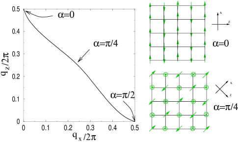
Figure 1: The ordering wave vector as the lattice is tilted by angle $\alpha$. As described in the text, for this situation a magnetic field is used to break the degeneracy between (${\cal N}=1$, ${\cal N}_{z}=-1,0,1$) states.

For the final example for the Mott insulating state, we consider a lattice in the $xz$-plane given by ${\bf a}_{1}=\cos(\alpha){\bf\hat{x}}+\sin(\alpha){\bf\hat{z}}$ and ${\bf a}_{2}=-\sin(\alpha){\bf\hat{x}}+\cos(\alpha){\bf\hat{z}}$. In addition, we consider breaking the degeneracy of the (${\cal N}=1$, ${\cal N}_{z}=-1,0,1$) states with an external static magnetic field in the $z$-direction which will introduce the term proportional to $BL_{z}$ into our hamiltonian. Preparing the system in a superposition of ${\cal N}=0$ and ${\cal N}=1,{\cal N}_{z}=1$ states, we note that because of this degeneracy breaking, there will be no mixing between other angular momentum states. That is, we can completely neglect the $t_{-1,0}$ states. This will give $\psi_{ix}=-i\psi_{iy}=e^{\varphi_{i}}/\sqrt{2}$ and $\psi_{z}=0$ which will confine our dipoles to rotate in the $xy$-plane as: $\langle{{\bf d}_{i}(t)}\rangle=d_{0}\cos(\varphi_{i}-2B_{e}t){\bf\hat{x}}+d_{0}\sin(\varphi_{i}-2B_{e}t){\bf\hat{y}}.$ The dipolar energy of this system is therefore

$$E_{\rm dip}=\frac{\gamma\sin^{2}(\theta)}{8}\sum_{i\neq j}\frac{\cos(\varphi_{i}-\varphi_{j})(1-\frac{3}{2}e_{ijx}^{2})}{|{\bf R}_{i}-{\bf R}_{j}|^{3}}.$$ (9)

We use the ansatz $\varphi_{i}={\bf q}\cdot{\bf R}_{i}+\varphi_{0}$ to find the minimum of this dipolar energy for a particular lattice defined by the angle $\alpha$, and the results are summarized in Fig. 1.

We now consider melting the Mott insulator, and entering the superfluid (SF) state. An interesting question to consider is what happens to the ordering wave vector as the Mott insulating state is melted? For instance, deep in the superfluid phase, we will have $q=0$ which is favorable for Bose-Einstein condensation while we saw that antiferromagnetic ordering is typically favored in the Mott insulating state by dipolar interactions. One possibility is that the wave vector interpolates smoothly between these two extremes as the hopping $J$ increases. Another possibility is that the molecules in the $s$ and $t$ states phase-separate. We will show below that both scenarios are possible depending on on-site energy parameters in our original hamiltonian. For simplicity, we restrict our attention to the third example we discussed above for the Mott insulating state which was a two dimensional lattice in the $xy$ plane prepared with $\sigma_{z}$ polarized light. For further simplicity, we take $\langle{N_{s}}\rangle=\langle{N_{t_{z}}}\rangle=N/2$. As we saw before, we can neglect populating the $t_{x}$ and $t_{y}$ states, and this phase has antiferromagnetic ${\bf q}=(\pi,\pi,0)$ order in the Mott insulating phase.

Allowing for noninteger occupation per site motivates the variational wave function

$$|{\Psi}\rangle=\prod_{i}\left(\sum_{n=0}^{\infty}\alpha_{n}\frac{(a_{i}^{\dagger})^{n}}{\sqrt{n!}}\right)|{0}\rangle$$ (10)

where $a_{i}^{\dagger}=\cos(\theta)e^{i{\bf p}_{s}\cdot{\bf R}_{i}}s_{i}^{\dagger}+\sin(\theta)e^{i{\bf p}_{t}\cdot{\bf R}_{i}}t_{iz}^{\dagger}$ and normalization requires $\sum_{n}|\alpha_{n}|^{2}=1$ (compare with (6)). As before, this wave function maximizes the dipole energy for a given site which is energetically favorable. We can now use a canonical transformation to write our original hamiltonian in terms of the boson operators $a_{i}^{\dagger}$ (defined above) and $b_{i}^{\dagger}=-\sin(\theta)e^{i{\bf p}_{s}\cdot{\bf R}_{i}}s_{i}^{\dagger}+\cos(\theta)e^{i{\bf p}_{t}\cdot{\bf R}_{i}}t_{iz}^{\dagger}$ (a new variable resulting from the transformation), and drop the terms which give zero when evaluated using the above variational wave function (10). This leads to the following single-site mean field hamiltonian

$${\cal H}_{\rm MF}= -2J \sum_{\alpha=x,y}\sqrt{\cos^{4}(\theta)+\sin^{4}(\theta)+2\cos^{2}(\theta)\sin^{2}(\theta)\cos(q_{\alpha})}\left(a^{\dagger}\langle{a}\rangle+a\langle{a^{\dagger}}\rangle-\langle{a^{\dagger}}\rangle\langle{a}\rangle\right)$$

$$+ \frac{\gamma}{4}\sin^{2}(2\theta)(2n_{a}\langle{n_{a}}\rangle-\langle{n_{a}}\rangle^{2})\sum_{{\bf R}_{i}\neq 0}\frac{\cos({\bf q}\cdot{\bf R}_{i})}{|{\bf R}_{i}|^{3}}+\frac{1}{2}Un_{a}(n_{a}-1)+\frac{1}{4}(V-U)\sin^{2}(2\theta)n_{a}(n_{a}-1)$$

where $n_{a}=a^{\dagger}a$ and we have already performed the minimization over the center of mass momentum ${\bf p}=({\bf p}_{t}+{\bf p}_{s})/2$. The ground state of this hamiltonian for fixed $\theta$ (relative concentrations) and ${\bf q}={\bf p}_{t}-{\bf p}_{s}$ (relative momentum) can be determined self-consistently in $\langle{a}\rangle$ and $\langle{n_{a}}\rangle$ through iteration numerically. The general approach will then be to minimize these ground state energies over $q_{x,y}\in[0,\pi]$ and $\theta\in[0,\pi/2]$. When the minimum occurs for $\theta\neq\pi/4$, phase separation will occur.

Figure 2: The phase diagram for $V=U$ (left) and $V=0$ (right). For both cases, the dipolar interaction strength was fixed at $\gamma=U/5$. Shown are the antiferromagnetic MI states with one and two bosons per site labeled MI1 and MI2. SF1 and SF2 correspond to superfluid states with partial and complete phase separation (described in text). SF3 is a superfluid phase with no phase separation which has an ordering wave vector that interpolates between the Mott insulating and deep superfluid regime.

The resulting phase diagrams are shown in Fig. 2. The Mott insulating phases are antiferromagnetically aligned and were discussed in the previous section. SF1 corresponds to partial phase separation where part of the lattice will have a larger concentration of $s$ molecules while the other part will have a higher concentration of $t$ molecules. Recall that phase separation will occur for when $\theta\neq\pi/4$ since we initially prepare the system to have equal populations of molecules in the $s$ and $t_{z}$ states. The region with more $s$ molecules will have $(p_{s})_{x,y}=0$ and $(p_{t})_{x,y}=\pi$. This will allow the more populated $s$ species to benefit maximally from BEC which prefers zero wave vector while still giving $q_{x,y}=\pi$ which is preferred for the dipole interaction. The similar situation holds for the region of the lattice with a higher concentration of $t_{z}$ molecules. SF2 corresponds to the case where the $s$ and $t_{z}$ molecules completely phase separate. Since the dipole interaction is negligible for this case, we will have $(p_{s})_{x,y}=(p_{t})_{x,y}=0$ which will favor BEC. Finally, SF3 corresponds to the case mentioned above where the wave vector $\bf q$ interpolates between the deep superfluid and Mott insulating states ($0<q_{x,y}<\pi$) for which no phase separation occurs ($\theta=\pi/4$).

In conclusion, we have shown that polar molecules prepared in a mixture of two rotational states can exhibit long-range dipolar interactions in the absence of an external electric field. We have described several novel Mott insulating and superfluid phases that can be realized as a result of such an interaction. Such states can be detected by Bragg scattering or by time-of-flight expansion Altman03 .

This work was supported by the NSF grant DMR-0132874 and career program, the Harvard-MIT CUA, and the Harvard-Smithsonian ITAMP. We thank B. Halperin, R. Krems, A. Polkovnikov, D.W. Wang, and P. Zoller for useful discussions.

Note added: When this manuscript was close to completion we became aware of a paper considering a similar system Micheli05 .

References

- (1) J. Doyle, B. Friedrich, R. V. Krems, and F. Masnou-Seeuws, Eur. Phys. J. D 31, 149 (2004).
- (2) K. Goral, K. Rzazewski, and T. Pfau, Phys. Rev. A 61, 051601 (2000).
- (3) J. Stuhler et. al, Phys. Rev. Lett. 95, 150406 (2005).
- (4) C. A. Stan et. al, Phys. Rev. Lett. 93, 143001 (2004).
- (5) S. Inouye et. al, Phys. Rev. Lett. 93, 183201 (2004).
- (6) J. M. Sage, S. Sainis, T. Bergeman, and D. DeMille, Phys. Rev. Lett. 94, 203001 (2005).
- (7) S. Yi and L. You, Phys. Rev. Lett. 92, 193201 (2004).
- (8) L. Santos, G. V. Shlyapnikov, P. Zoller, and M. Lewenstein, Phys. Rev. Lett. 85, 1791 (2000).
- (9) D. DeMille, Phys. Rev. Lett. 88, 067901 (2002).
- (10) K. Goral, L. Santos, and M. Lewenstein, Phys. Rev. Lett. 88, 170406 (2002).
- (11) M. G. Moore and H. R. Sadeghpour, Phys. Rev. A 67, 041603 (2003).
- (12) A. Micheli, G. Brennen, and P. Zoller, eprint quant-ph/0512222.
- (13) O. Mandel et. al, Nature 425, 937 (2003).
- (14) L.-M. Duan, E. Demler, and M. Lukin, Phys. Rev. Lett. 91, 090402 (2003).
- (15) A. Kuklov, N. Prokof’ev, and B. Svistunov, Phys. Rev. Lett. 92, 050402 (2004).
- (16) A. Isacsson, M.-C. Cha, K. Sengupta, and S. M. Girvin, Phys. Rev. B 72, 184507 (2005).
- (17) B. Damski et. al, Phys. Rev. Lett. 95, 060403 (2005).
- (18) X.-L. Deng, D. Porras, and J. I. Cirac, eprint cond-mat/0509197.
- (19) J. A. Sauer, Phys. Rev. 57, 142 (1940).
- (20) J. M. Luttinger and L. Tisza, Phys. Rev. 70, 954 (1946).
- (21) R. Moessner and S. L. Sondhi, Phys. Rev. B 68, 054405 (2003).
- (22) The rotational relaxation can be greatly reduced in an optical lattice, similar to the inelastic losses in the atomic case. It can completely eliminated in the 1 atom Mott case and suppressed in a deep lattice.
- (23) S. Yi and L. You, Phys. Rev. Lett. 92, 193201 (2004).
- (24) See, for instance, chapter 1 and 2 of K. Huang, Statistical Mechanics (John Wiley and Sons, 1987).
- (25) E. Altman, E. Demler, and M. Lukin, Phys. Rev. A 70, 013603 (2004).