Interplay between parallel and diagonal electronic nematic phases in interacting systems

Abstract

An electronic nematic phase can be classified by a spontaneously broken discrete rotational symmetry of a host lattice. In a square lattice, there are two distinct nematic phases. The parallel nematic phase breaks $x$ and $y$ symmetry, while the diagonal nematic phase breaks the diagonal $(x+y)$ and anti-diagonal $(x-y)$ symmetry. We investigate the interplay between the parallel and diagonal nematic orders using mean field theory. We found that the nematic phases compete with each other, while they coexist in a finite window of parameter space. The quantum critical point between the diagonal nematic and isotropic phases exists, and its location in a phase diagram depends on the topology of the Fermi surface. We discuss the implication of our results in the context of neutron scattering and Raman spectroscopy measurements on La_2-xSr_xCuO₄.

I Introduction

Recently, there has been a great effort to understand intrinsic phases of a doped Mott insulator in the context of high temperature superconductors. It has been proposed that quantum fluctuations of a Mott insulator introduced by hole doping lead to intermediate forms of matter, dubbed as electronic smectic and nematic phases.Kivelson et al. (1998, 2003) In analogy to classical liquid crystals, the smectic phase breaks translational symmetry along one direction, while the nematic phase breaks rotational symmetry.

The evidence of such inhomogeneous and/or anisotropic liquid phases has been found in strongly correlated electron systems. Tranquada et al. (1995); Mori et al. (1998); Lilly et al. (1999); Du et al. (1999); Cooper et al. (2002); Ando et al. (2002) In particular, the clear evidence of a nematic liquid phase has been reported in two-dimensional electron gases in magnetic fields in ultra-clean samples.Lilly et al. (1999) The observed strong anisotropy of longitudinal resistivity has been explained by the onset of a nematic phase at low temperatures. A recent theoretical study of the nematic phase using a quadrupolar interaction, $F_{2}$, has offered non-Fermi liquid behavior in the nematic phase as well as near the quantum critical point.Oganesyan et al. (2001) This is originated from large fluctuations of the overdamped collective modes within the RPA theory. A non-perturbative approach using higher dimensional bosonization reproduced the quantum critical behavior with the dynamical exponent of $z=3$, and verified the non-Fermi liquid behavior in the nematic phase. Lawler et al. (2005)

However, it was shown that the nature of phase transition of the model with the quadrupolar interaction is quite different when we take into account an underlying square lattice.Kee et al. (2003); Khavkine et al. (2004) On a lattice, a nematic phase can be achieved via a spontaneously broken point-group symmetry due to interactions between electrons. For example, it can break $x$ and $y$ symmetry of a square lattice. An essential consequence of nematic order is a deformation of a Fermi surface. It was shown that the transition from isotropic liquid to the nematic phase which breaks $x$ and $y$ symmetry of the square lattice is strongly first order at low temperatures. The nematic order parameter jumps at the transition to avoid the van Hove singularity, thus suppressing the Lifshitz transition. The transition takes place at arbitrarily small attractive quadrupolar interaction at the van Hove band filling. The transition changes to a continuous one at a finite temperature, but is not affected by either the next neighbor hopping, $t^{\prime}$, nor small dispersion in the third direction.

In this paper, we study two distinct nematic phases in the square lattice, and investigate the interplay between them. The parallel nematic phase previously studiedKhavkine et al. (2004) breaks a symmetry between $x$ and $y$, while the diagonal nematic phase breaks a symmetry between two diagonal, $(x+y)$ and $(x-y)$ directions. The order parameter associated with the parallel $(\Delta)$ and diagonal $(\Delta^{\prime})$ nematic phases are defined as follows:

$$\Delta = F_{2}\sum_{{\bf k}}(\cos k_{x}-\cos k_{y})\left\langle c_{\bf k}^{\dagger}c_{\bf k}\right\rangle,$$

$$\Delta^{\prime} = F_{2}^{\prime}\sum_{{\bf k}}(2\sin k_{x}\sin k_{y})\left\langle c_{\bf k}^{\dagger}c_{\bf k}\right\rangle.$$ (1)

It was shown that $\Delta^{\prime}$ is always 0 for a given quadrupolar interaction $F_{2}$, which implies that a preferred direction for electron momenta has been selected to be parallel to the crystal axes. Here we study the interplay between parallel and diagonal nematic phases using a phenomenological model with two different strengths of interactions, $F_{2}$ and $F_{2}^{\prime}$ for the parallel and diagonal nematic orders, respectively. We find that the transition to the diagonal nematic ordered state from isotropic liquid phase occurs above a critical value of interaction $F_{2}^{\prime}$, and it is second order as a function of chemical potential. The competition between the diagonal and parallel nematic phases leads to suppression of the strengths of both phases, while they coexist in a finite window of chemical potential.

The paper is organized as follows. We describe the effective model Hamiltonian for the nematic order in section II. The mean field analysis at zero temperature is given in section III. The effect of $t^{\prime}$ is also presented. We discuss the implication of our results and compare with neutron scattering and Raman spectroscopy measurements on La_2-xSr_xCuO₄ in section IV. We provide the summary of our findings and future works in the last section.

II Hamiltonian for Nematic orders

Within a weak-coupling theory, the instability toward a Fermi surface deformation, often referred to as Pomeranchuk instability,Pomeranchuk (1958) has been discussed in a Fermi liquid, $t-J$ model, Hubbard model, and the extended Hubbard model.Nilsson and Neto (2005); Yamase and Kohno (2000); Halboth and Metzner (2000); Hankevych et al. (2002); Neumayr and Metzner (2003) It was shown that a strongly nematic phase (quasi-1D) is stable in a strong coupling limit of the two dimensional Emery model.Kivelson et al. (2004) A phenomenological model with quadrupolar density interaction in the continuum case was introduced in Ref.Oganesyan et al., 2001, and it was extended to the square lattice in Ref.Kee et al., 2003; Yamase et al., 2005.

The quadrupolar density interaction involves two distinct nematic phases in the square lattice. For the parallel nematic phase, the Fermi surface expands along $k_{x}(k_{y})$-axis and shrinks along the $k_{y}(k_{x})$-axis. On the other hand, for the diagonal nematic phase, the Fermi surface expands along $(k_{x}+k_{y})$ and shrinks along the $(k_{x}-k_{y})$ directions (or vice versa). While the mean field study for the case of $F_{2}({\bf q})=F_{2}^{\prime}({\bf q})$ showed no preference of diagonal order,Kee et al. (2003); Khavkine et al. (2004) the various experiments in cuprates indicates possibility of both parallel and diagonal fluctuating stripes.Wakimoto et al. (2000); Fujita et al. (2002); Tassini et al. (2005) Here we consider the following model Hamiltonian which offers us to study the interplay between the parallel and diagonal nematic phases.

$$H = \sum_{{\bf k}\sigma}\varepsilon_{\bf k}c_{{\bf k}\sigma}^{\dagger}c_{{\bf k}\sigma}$$ (2)

$$-\sum_{{\bf k}{\bf k}^{\prime}{\bf q}\sigma\sigma^{\prime}}\left[F_{2}({\bf q})\zeta_{1}({\bf k})\zeta_{1}({\bf k}^{\prime})+F_{2}^{\prime}({\bf q})\zeta_{2}({\bf k})\zeta_{2}({\bf k}^{\prime})\right]$$

$$\times c_{{\bf k}+\frac{{\bf q}}{2}\sigma}^{\dagger}c_{{\bf k}^{\prime}-\frac{{\bf q}}{2}\sigma^{\prime}}^{\dagger}c_{{\bf k}^{\prime}+\frac{{\bf q}}{2}\sigma^{\prime}}c_{{\bf k}-\frac{{\bf q}}{2}\sigma},$$

where $F_{2}({\bf q})$ and $F_{2}^{\prime}({\bf q})$ are given as follows.

$$F_{2}({\bf q})=\frac{F_{2}}{1+\kappa q^{2}},~{}~{}~{}~{}~{}F_{2}^{\prime}({\bf q})=\frac{F_{2}^{\prime}}{1+\kappa^{\prime}q^{2}}.$$ (3)

Here $\epsilon({\bf k})$, $\zeta_{1}({\bf k})$, and $\zeta_{2}({\bf k})$ are given by

$$\varepsilon({\bf k}) = -t(\cos k_{x}+\cos k_{y})-2t^{\prime}\cos k_{x}\cos k_{y}-\mu$$ (4)

$$\zeta_{1}({\bf k}) = \cos k_{x}-\cos k_{y}$$ (5)

$$\zeta_{2}({\bf k}) = 2\sin k_{x}\sin k_{y}.$$ (6)

The mean field Hamiltonian for the uniform nematic orders is written as

$$H_{\mbox{\scriptsize mean}}=\sum_{\bf k}\tilde{\varepsilon}_{\bf k}c_{\bf k}^{\dagger}c_{\bf k}+\frac{|\Delta|^{2}}{2F_{2}}+\frac{|\Delta^{\prime}|^{2}}{2F_{2}^{\prime}},$$ (7)

where

$$\tilde{\varepsilon}_{\bf k}=\varepsilon_{\bf k}-\Delta\zeta_{1}({\bf k})-\Delta^{\prime}\zeta_{2}({\bf k}).$$ (8)

Here $\Delta$ and $\Delta^{\prime}$ measure the strength of the broken $x$ vs. $y$ and $(x+y)$ vs. $(x-y)$ symmetries, respectively.

$$\Delta = F_{2}\sum_{\bf k}\left(\cos k_{x}-\cos k_{y}\right)\theta(-\tilde{\varepsilon})$$

$$\Delta^{\prime} = F_{2}^{\prime}\sum_{\bf k}\left(2\sin k_{x}\sin k_{y}\right)\theta(-\tilde{\varepsilon})$$ (9)

We compute the free energy using mean field theory, and discuss the phase transition in the following section.

III Phase transition of Nematic orders

III.1 Free energy and Nematic order parameters

The mean field free energy at zero temperature is given by

$$F_{0}(\mu,\Delta,\Delta^{\prime})=\sum_{\bf k}\tilde{\varepsilon}\theta(-\tilde{\varepsilon})+\frac{\Delta^{2}}{2F_{2}}+\frac{{\Delta^{\prime}}^{2}}{2F_{2}^{\prime}}$$ (10)

where $\theta(\epsilon)$ is step function. Using adaptive 2-dimensional integration,Henk (2001) we obtain the free energy in terms of chemical potential and the nematic orders, $\Delta$ and $\Delta^{\prime}$ Here, we ignored the next-nearest hopping $t^{\prime}$, but we will consider it later in sec. III.4.

To understand the nature of the transition between the diagonal nematic and isotropic phases, let us first set $F_{2}=0$. Fig. 1 shows the free energy as a function of the diagonal nematic order, $F(\Delta^{\prime})$ for several values of chemical potential. It is clear that the transition from the diagonal nematic phase to the isotropic phase is second order; the diagonal order parameter as a function of chemical potential changes continuously. We found that $\Delta^{\prime}$ has finite value only when $F_{2}^{\prime}$ exceeds some critical value $F_{2c}^{\prime}$ which depends on the value of $\Delta$. For the case of $F_{2}=0$, $F_{2c}^{\prime}N_{0}$ is $0.1876$ from our numerical calculation. Fig. 2 shows that there is no minimum in the free energy except $\Delta^{\prime}=0$ for $F_{2}^{\prime}N_{0}<F_{2c}^{\prime}N_{0}=0.1876$.

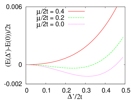
Figure 1: Free energy as a function of $\Delta^{\prime}$ for various values of chemical potential and $F_{2}^{\prime}N_{0}=0.2077$. The value of free energy has been rescaled to $0$ at $\Delta^{\prime}=0$.

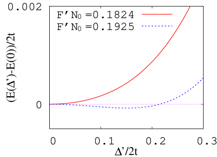
Figure 2: Free energy as a function of $\Delta^{\prime}$ for several values of the interaction, $F_{2}^{\prime}$ and $\mu=0$. The free energy has minimum at a finite $\Delta^{\prime}$ only when $F_{2}^{\prime}$ is larger than a critical value. Ihe value of free energy has been rescaled to $0$ at $\Delta^{\prime}=0$.

We now turn on $F_{2}$ to understand the interplay between parallel and diagonal nematic orders. The behaviors of nematic order parameters as one varies $F_{2}/F_{2}^{\prime}$ are obtained by solving the self-consistent equation, (9). All possible types of phase diagram for $\Delta$ and $\Delta^{\prime}$ are summarized in Fig. 3. As we increase $F_{2}$, the parallel nematic order suddenly develops near $\mu=0$ where the van Hove singularity exists. This is illustrated in Fig. 3 (b). The suppression of diagonal nematic order due to the development of the parallel nematic order is clearly observed as well. However, the region of finite $\Delta^{\prime}$ does not change as long as $F_{2}^{\prime}$ is fixed. As shown in Fig. 3 (c), a further increase of $F_{2}$ leads to a wider region of the parallel nematic order, which now totally suppresses the diagonal nematic order inside its territory. However, it does not take over the whole region of the diagonal nematic order. A finite $\Delta^{\prime}$ region outside the territory of the parallel nematic order is still found. A further increase of $F_{2}$ eventually removes the diagonal nematic phase in the picture as shown in Fig. 3 (d).

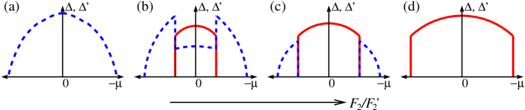
Figure 3: All types of phase diagrams for $\Delta$ and $\Delta^{\prime}$ as a function of chemical potential obtained by tuning the ratio between two interactions $F_{2}/F_{2}^{\prime}$, and $t^{\prime}=0$. The solid and dashed lines denote $\Delta$ and $\Delta^{\prime}$, respectively. See the main text for the discussion on (a) -(d).

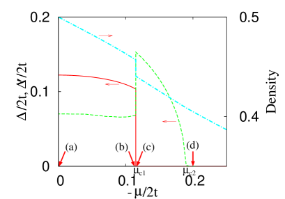
Figure 4: Nematic orders and electron density vs. chemical potential for $F_{2}N_{0}=0.1$ and $F_{2}^{\prime}N_{0}=0.196$. The solid and dashed lines denote $\Delta$ and $\Delta^{\prime}$, respectively. The dot-dashed line denotes the electron density. The arrows labeled (a) to (d) are the values of chemical potentials used in Fig. 5 and the discussion in the main text.

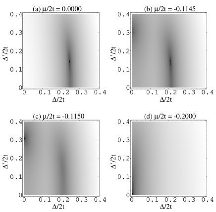
Figure 5: The density plot of free energy as functions of $\Delta$ and $\Delta^{\prime}$ for several values of chemical potentials indicated by the arrows in Fig. 4, and for given values of interactions, $F_{2}N_{0}=0.1$ and $F_{2}^{\prime}N_{0}=0.196$. Darker is lower free energy. The minimum points for each figure denote the equilibrium values of $\Delta$ and $\Delta^{\prime}$. The discussion on (a) - (d) can be found in the main text.

It is worthwhile to emphasize the following important features of the nematic orders in the coexistence regime. The region where the diagonal nematic order is finite is always wider than that of the parallel nematic order, if it ever exists. As shown in Fig. 4, $\Delta$ has a finite value for $|\mu/2t|<0.115$, and $\Delta^{\prime}$ for $|\mu/2t|<0.19$. In other words, the critical chemical potential for $\Delta^{\prime}$, $\mu_{c2}$ is always bigger than that for $\Delta$, $\mu_{c1}$. At $\mu=\mu_{c1}$, $\Delta$ drops to zero discontinuously and the electron density also changes abruptly, which shows the first order phase transition. When $\Delta$ goes to zero at $\mu_{c1}$, $\Delta^{\prime}$ gets enhanced from $0.0679$ to $0.1529$ (in unit of $2t$). We found that the region of $\Delta$ is also shrunk due to finite $\Delta^{\prime}$, which is further discussed in the following subsection. As the chemical potential approaches $\mu_{c2}$, $\Delta^{\prime}$ gradually goes to zero reflecting the second order phase transition. At this transition, the electron density varies continuously and shows only the tiny change of its slope.

We show the behavior of free energies around the critical chemical potentials, to highlight these two distinctive phase transitions at $\mu_{c1}$ and $\mu_{c2}$ in Fig. 5. Fig. 5 (a) shows that the minimum of the free energy for $\mu/2t=0$ occurs at finite $\Delta$ and $\Delta^{\prime}$. As the chemical potential approaches to the first critical point, $|\mu_{c1}/2t|=0.115$ another minimum point begins to develop at $\Delta/2t=0$ and $\Delta^{\prime}/2t=0.1529$ as shown in Fig. 5 (b). At the critical point $\mu_{c1}$, there exist two clear minima as shown in Fig. 5 (c). The global minimum of $(\frac{\Delta}{2t},\frac{\Delta^{\prime}}{2t})$ is changed from $(0.1035,0.0679)$ to $(0,0.1529)$ as $|\mu/2t|$ crosses the critical point, $0.115$. A further increase of $\mu$ finds a unique minimum at $D=D^{\prime}=0$ as shown in Fig. 5 (d).

III.2 Phenomenological Analysis of two competing orders

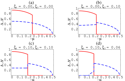
Figure 6: Order parameters determined from the Ginzburg-Landau equation of (III.2) for various values of $\xi_{1}$ and $\xi_{2}$. The other parameters are $\alpha=0.1$, $\beta_{0}=4.0$, $\gamma=1.0$, $\alpha_{0}^{\prime}=1.0$, $\beta^{\prime}=1.0$, $\gamma^{\prime}=0.0$, $\xi_{3}=0.0$, $\mu_{c1}=0.25$, and $\mu_{c2}=0.5$. The solid and dashed lines denote $\Delta$ and $\Delta^{\prime}$, respectively.

To get an insight on competing two nematic orders, we analyze the following Ginzburg-Landau (GL) free energy.

$$F_{\mbox{\scriptsize GL}}(\Delta,\Delta^{\prime}) = \frac{\alpha}{2}\Delta^{2}+\frac{\beta(\mu)}{4}\Delta^{4}+\frac{\gamma}{6}\Delta^{6}$$

$$+\frac{\alpha^{\prime}(\mu)}{2}{\Delta^{\prime}}^{2}+\frac{\beta^{\prime}}{4}{\Delta^{\prime}}^{4}+\frac{\gamma^{\prime}}{6}{\Delta^{\prime}}^{6}$$

$$+\frac{\xi_{1}}{2}{\Delta}^{2}{\Delta^{\prime}}^{2}+\frac{\xi_{2}}{2}{\Delta}^{4}{\Delta^{\prime}}^{2}+\frac{\xi_{3}}{2}{\Delta}^{2}{\Delta^{\prime}}^{4}.$$

We expand the free energy in terms of the order parameters up to the 6-th orders, since the parallel nematic order denoted by $\Delta$ shows the first order transition. We set $\gamma^{\prime}=\xi_{3}=0$ for a simplicity, because different values of $g^{\prime}$ and $\xi_{3}$ do not affect our qualitative analysis. We introduce positive mutual interaction coefficients ($\xi_{1}>0$ and $\xi_{2}>0$) between two orders, since the two nematic orders suppress each other. Here $\alpha^{\prime}$($\beta$) changes its sign as it crosses the critical chemical potential $\mu_{c2}$($\mu_{c1}$), and it is an even function of the chemical potential due to a particle-hole symmetry. We consider the following form of $\beta(\mu)$ and $\alpha^{\prime}(\mu)$.

$$\beta(\mu) = \beta_{0}(\mu^{2}-\mu_{c1}^{2})-\sqrt{\frac{16\alpha\gamma}{3}},~{}~{}~{}\mbox{and }$$ (12)

$$\alpha^{\prime}(\mu) = \alpha_{0}^{\prime}(\mu^{2}-\mu_{c2}^{2}).$$ (13)

The order parameters are determined by solving the following equations, and shown in Fig. 6 for several values of $\xi_{1}$ and $\xi_{2}$.

$$\!\!0 \!\!=\!\! \left[\alpha\!\!+\xi_{1}{\Delta^{\prime}}^{2}\!\!+\left(\beta(\mu)+2\xi_{2}{\Delta^{\prime}}^{2}\right)\Delta^{2}\!\!+\gamma\Delta^{4}\right]\!\!\Delta$$ (14)

$$\!\!0 \!\!=\!\! \left[\alpha^{\prime}(\mu)+\xi_{1}\Delta^{2}\!\!+\xi_{2}\Delta^{4}\!\!+\beta^{\prime}{\Delta^{\prime}}^{2}\right]\Delta^{\prime}$$ (15)

The amplitude of $\Delta$ is not much affected due to the mutual interaction term. However, the critical chemical potential, $\mu_{c1}$ is shifted in such a way that the region of the parallel nematic phase becomes narrower. The modified critical chemical potential, $\tilde{\mu}_{c1}$ is given by the following equation.

$$\tilde{\mu}_{c1}=\sqrt{\mu_{c1}-\sqrt{\frac{16\alpha\gamma}{3\beta_{0}^{2}}}\left(\sqrt{1+\frac{\xi_{1}{\Delta^{\prime}}^{2}}{\alpha}}-1\right)-\frac{2\xi_{2}{\Delta^{\prime}}^{2}}{\beta_{0}}}.$$ (16)

On the other hand, the magnitude of $\Delta^{\prime}$ is suppressed due to finite $\Delta$, and it is modified as follows.

$$\Delta^{\prime}=\sqrt{\frac{\alpha_{0}^{\prime}(\mu_{c2}^{2}-\mu^{2})-\xi_{1}\Delta^{2}-\xi_{2}\Delta^{4}}{\beta^{\prime}}}$$ (17)

The critical chemical potential, $\mu_{c2}$ is not affected as long as $\mu_{c2}>\tilde{\mu}_{c1}$. Our GL analysis captures the key features of our results presented in sec. III.1. They suppress each other in qualitatively different ways. The parallel nematic order suppresses the amplitude of the diagonal nematic order, while the window of the diagonal nematic order is not affected when they coexist. On the other hand, the diagonal nematic order shrinks the parallel nematic order region, but hardly suppresses the amplitude of $\Delta$.

III.3 Fermi surface and density of states

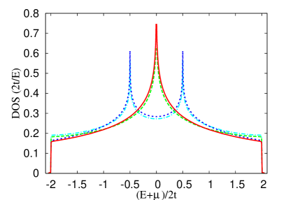
Figure 7: Density of states for various values of $\Delta$ and $\Delta^{\prime}$. The solid line is for $(\Delta/(2t),\Delta^{\prime}/(2t))=(0,0)$, the dashed for $(0,0.25)$, the dotted for $(0.25,0)$, and the dot-dashed for $(0.25,0.25)$. A finite $\Delta$ splits the van Hove singularity at $E=-\mu$ into two peaks, while $\Delta^{\prime}$ shows the minor effect on the density of states.

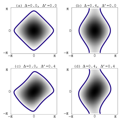
Figure 8: Fermi surface for several values of $\Delta$ and $\Delta^{\prime}$. The deformation of the original Fermi surface shown in (a) along the parallel (diagonal) axes of the lattice is due to the parallel (diagonal) nematic order. Examples of Fermi surface for the parallel and diagonal nematic order phases shown in (b) and (c), respectively. An example of Fermi surface for finite $\Delta$ and $\Delta^{\prime}$ is shown in (d).

To understand the nature of the phase transition, we investigate effects of nematic orders on the density of states (DOS) and Fermi surface. The DOS for several values of $\Delta$ and $\Delta^{\prime}$ is shown in in Fig. 7. Without the nematic orders, DOS has a singularity at $E+\mu=0$ originated from the van Hove singularity (VHS). It was shown that the development of $\Delta$ (the dotted line) leads to a dramatic change in DOS. The parallel nematic order splits the VHS into two peaks occurring near the van Hove filling. As a result, the free energy is lowered.Khavkine et al. (2004) This feature is inherited from the logarithmic singularity in the free energy. (See ref.Khavkine et al., 2004 for detail.) On the other hand, $\Delta^{\prime}$ is nothing to do with the VHS as shown in Fig. 7. The peak from VHS is not affected by a development of $\Delta^{\prime}$. The DOS has only minor change due to $\Delta^{\prime}$, which is a slight enhancement near the band edge and suppression near the center of the band. Therefore, the free energy develops a minimum continuously from $\Delta^{\prime}=0$ to a finite $\Delta^{\prime}$, as one changes $\mu$, thus the transition between isotropic and the diagonal nematic phases is second order.

One of important consequences of the nematic order is a deformation of the Fermi surface. The deformation of Fermi surfaces for various values of $\Delta$ and $\Delta^{\prime}$ are shown in Fig. 8. Fig. 8 (a) shows the undeformed Fermi surface to make comparison with (b)-(d). A finite parallel nematic order, $\Delta$ squeezes the Fermi surface along a parallel axis of the lattice as shown in Fig. 8 (b). For example, it shrinks the Fermi surface in $k_{x}$-direction and expands it in $k_{y}$-direction, or reverse way. On the other hand, the diagonal nematic order $\Delta^{\prime}$ deforms the Fermi surface along a diagonal axis of the lattice as shown in Fig. 8 (c). For example, it shrinks the Fermi surface in $(k_{x}-k_{y})$-direction and extend in $(k_{x}+k_{y})$-direction, and vise versa. The discontinuous change of $\Delta$ related to the van Hove singularity leads to a dramatic change in the shape of Fermi surface as shown in Fig. 8 (b). On the other hand, the deformation along the diagonal direction develops continuously, as one changes $\mu$. It is important to note that $D^{\prime}$ does not affect four points on the Fermi surface, $(\pm k_{Fx},0)$ and $(0,\pm k_{Fy})$, which eventually lead to the van Hove singularity at the van Hove filling and the formation of the parallel nematic phase inside the diagonal nematic phase.

III.4 Effects of next-nearest hopping

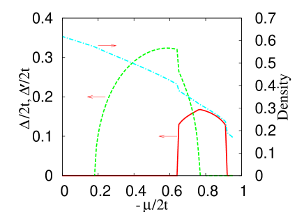
Figure 9: Nematic orders and electron density vs. chemical potential for $t^{\prime}=-0.4t$, $F_{2}N_{0}=0.1$ and $F_{2}^{\prime}N_{0}=0.196$. The solid and dashed lines denote $\Delta$ and $\Delta^{\prime}$, respectively. The dot-dashed line indicates the electron density.

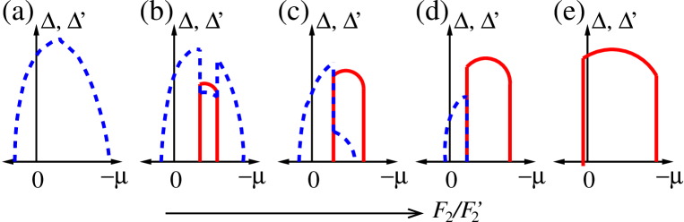
Figure 10: Various types of phase diagrams for $\Delta$ and $\Delta^{\prime}$ with the next-nearest-hopping $t^{\prime}$. The solid line is designated for $\Delta$ and the dashed line for $\Delta^{\prime}$. A negative $t^{\prime}$ shifts both $\Delta$ and $\Delta^{\prime}$ toward hole-doped region. (a) $F_{2}=0$ and $F_{2}^{\prime}>0$. (b) A small increase of $F_{2}$ leads to a development of the parallel nematic phase inside the diagonal nematic phase region. (c) A further increase of $F_{2}$ increases the parallel nematic phase region, thus suppresses the region of diagonal nematic phase. (d) the diagonal nematic order is totally suppressed within the region of parallel nematic phase, while it still survives outside the region. (e) The parallel nematic order eventually removes the diagonal nematic order by expanding its region.

In this section, we introduce the next-nearest hopping integral, $t^{\prime}$ in (4), which breaks a particle-hole symmetry. We found that a negative sign of $t^{\prime}$ shifts the region of nematic phases toward hole-doped region. However, since the parallel nematic order always appears near a VHS, while the diagonal nematic order is not directly affected by a VHS, we expect that the region of parallel nematic and diagonal nematic phases will be shifted in a slightly different way, as we increase $t^{\prime}$. On the other hand, qualitative features such as nature of phase transition are not affected by a finite $t^{\prime}$.

Fig. 9 shows a phase diagram for $t^{\prime}=-0.4t$. The parallel nematic order is shifted more to the hole doped region than the diagonal nematic order. At the half-filling, only the diagonal nematic order is finite. As we increase $|\mu|$ (or hole concentration), the coexistence of two nematic phases appears. A further increase of $|\mu|$ leads to a suppression of the diagonal nematic order, while the parallel nematic phase gets stronger. Finally only the parallel nematic order remains, which eventually disappears in the phase diagram, as the hole concentration is increased. The nematic order rotates from the parallel order to the diagonal order, as we increase hole doping concentration, and two phases coexist near the boundary. This feature resembles the rotation of charge fluctuations associated with $B_{2g}$ channel to $B_{1g}$ channel by increasing doping concentration which was reported in the Raman spectroscopy measurement on La_2-xSr_xCuO₄ (LSCO).Tassini et al. (2005) The rotation of spin modulation by changing doping concentration in LSCO was also found in elastic neutron scattering patterns.Fujita et al. (2002) Elastic neutron scattering studies on LSCO showed one-dimensional spin modulation along the orthorhomic $b$-axis in lower doping concentrations, and another type of spin modulation parallel to the tetragonal axes in high doping concentrations. The coexistence of two types of spin modulations near the boundary was also reported.Fujita et al. (2002) While direct comparisons to the neutron scattering patterns and/or Raman spectroscopy data require further theoretical studies on corresponding susceptibilities in the nematic phases, we expect that the behavior of Fermi surface deformation within our model offers a consistent picture compared with the experimental observations.

Fig. 10 summarizes the typical types of phase diagrams for two nematic orders with the next-nearest hopping. For a finite negative $t^{\prime}$, both $\Delta(\mu)$ and $\Delta^{\prime}(\mu)$ are shifted to hole-doped region but in a slightly different way, as we discussed. When they coexist, the maxima of two nematic phases do not coincide as shown in Fig. 3 due to their different $t^{\prime}$ dependences. However, the qualitative behaviors of competition between two nematic orders are similar to the case without $t^{\prime}$ presented in the sec. III A.

IV Discussion and Summary

A quantum analog of classical liquid crystal in terms of broken symmetry has been discussed in the context of a doped Mott insulator.Kivelson et al. (2003) Among the electronic liquid crystal phases, nematic phases can be viewed as fluctuating stripes whose segments are fluctuating in time but oriented in a particular direction, and hence breaks orientational symmetry.

Recent neutron scattering measurements of detwinned YBa₂Cu₃O_7-δ have indicated a possible existence of two dimensional anisotropic liquid crystalline phase in high temperature cuprates.Hinkov et al. (2004); Stock et al. (2005); Kao and Kee (2005) Extensive neutron scattering measurements of La_2-xSr_xCuO₄ in a wide range of doping have also revealed the doping dependence of the static or quasi-static spin ordering in insulating and superconducting phase.Wakimoto et al. (2000); Fujita et al. (2002) An interesting observation is that the orientation of the spin modulation depends on the doping concentration. It was found that the spin modulation vector is diagonal to the Cu-O bond in the insulating spin glass phase, while inside the superconducting phase it is parallel to the tetragonal axes. These two types of spin modulation coexist near the boundary between the insulating and superconducting phases. Such a one-dimensional nature of the spin correlations is consistent with a stripe-like ordering of the holes in the CuO₂ planes.Tranquada et al. (1995)

Inelastic light-scattering spectra of underdoped La_2-xSr_xCuO₄ single crystals showed additional Drude-like responses in $B_{2g}$ and $B_{1g}$ channels for $x=0.02$ to $x=0.10$, respectively.Tassini et al. (2005) This was interpreted as experimental evidence of fluctuating charge stripes whose orientation rotates from diagonal to parallel by varying the doping concentration of Sr from $x=0.02$ to $x=0.10$.Tassini et al. (2005) More extensive studies for various doping concentrations will be required to determine the coexistence of two types of charge modulations. While direct comparisons to these experimental data require theoretical studies on corresponding susceptibilities, we expect that our phenomenological model provides a possible explanation of the rotation of the spin and charge modulations observed in LSCO.

In summary, we have studied the interplay between parallel and diagonal nematic phases using the phenomenological model Hamiltonian within mean field theory. We found that the parallel and diagonal nematic phases compete each other – the parallel nematic order suppresses the amplitude of the diagonal nematic order, while the diagonal nematic order shrinks the window of the parallel nematic order. However, they still coexist in a finite window of parameter space. The transition to the parallel nematic phase is strongly first order, while the diagonal nematic phases shows the continuous transition to the isotropic phase. Effects of quantum fluctuation of the diagonal nematic order parameter on various quantities near a quantum critical point are the subjects of future studies, and the single particle self-energy correction due to the fluctuation of a collective mode will be presented elsewhere.Puetter and et al (2005)