Quantum Monte Carlo Study of Strongly Correlated Electrons:
Cellular Dynamical Mean-Field Theory

Abstract

We study the Hubbard model using the Cellular Dynamical Mean-Field Theory (CDMFT) with quantum Monte Carlo (QMC) simulations. We present the algorithmic details of CDMFT with the Hirsch-Fye QMC method for the solution of the self-consistently embedded quantum cluster problem. We use the one- and two-dimensional half-filled Hubbard model to gauge the performance of CDMFT+QMC particularly for small clusters by comparing with the exact results and also with other quantum cluster methods. We calculate single-particle Green’s functions and self-energies on small clusters to study their size dependence in one- and two-dimensions. It is shown that in one dimension, CDMFT with two sites in the cluster is already able to describe with high accuracy the evolution of the density as a function of the chemical potential and the compressibility divergence at the Mott transition, in good agreement with the exact Bethe ansatz result. With increasing $U$ the result on small clusters rapidly approaches that of the infinite size cluster. Large scattering rate and a positive slope in the real part of the self-energy in one-dimension suggest that the system is a non-Fermi liquid for all the parameters studied here. In two-dimensions, at intermediate to strong coupling, even the smallest cluster ($N_{c}=2\times 2$) accounts for more than $95\%$ of the correlation effect of the infinite-size cluster in the single particle spectrum, suggesting that some of the important problems in strongly correlated electron systems may be studied highly accurately with a reasonable computational effort. Finally, as an application that is sensitive to details of correlations, we show that CDMFT+QMC can describe spin-charge separated Luttinger liquid physics in one dimension. The spinon and holon branches appear only for sufficiently large system sizes.

I Introduction

Strongly correlated electron systems realized in organic conductors, heavy fermion compounds, transition metal oxides, and more recently high temperature superconductors continue to challenge our understanding. Various anomalous behaviors observed in these materials cannot be well understood within conventional theoretical tools based on a Fermi liquid picture or a perturbative scheme. Because these intriguing features appear in a non-perturbative regime, numerical methods have played a key role. Exact diagonalization (ED) and Quantum Monte Carlo (QMC) simulations Dagotto:1994 are amongst the most popular approaches. However, severe limitations due to small lattice size in ED and a minus sign problem in QMC at low temperatures make it difficult to extract reliable low-energy physics from these calculations.

Recently, alternative approaches HTJPK:1998 ; SPP:2000 ; LK:2000 ; KSPB:2001 ; P:2003 ; MJPH:2004 , such as the Dynamical Cluster Approximation, Cluster Perturbation Theory, the Self-Energy Functional Approach and Cellular Dynamical Mean-Filed Theory (CDMFT) have been developed and have already given some promising results. Most of these quantum cluster methods generalize the single-site Dynamical Mean Field Theory (DMFT) GK:1992 ; Jarrell:1992 ; GKKR:1996 to incorporate short-range spatial correlations explicitly. In fact the DMFT has provided the first unified scenario for the long standing problem of the Mott transition in the Hubbard model, completely characterizing the criticality associated with this transition in infinite dimension or when spatial correlations are negligible. In spite of its great success in answering some of the challenging questions in strongly correlated electron systems, its limitation has been also recognized in understanding low dimensional electronic systems such as high temperature superconductors for instance. In particular, the observed normal state pseudogap in underdoped cuprates TS:1999 is in sharp contrast with the prediction of DMFT in which any slight doping into the half-filled band always leads to a Fermi liquid. Many of the discrepancies are traced back to the neglect of short-range correlations in DMFT. The main objective of these alternative approaches is to describe short-range spatial correlations explicitly and to study the physics that emerges. CDMFT has been recently applied to the Hubbard model using ED as cluster solver at zero temperature, as we will discuss later, and to the model for layered organic conductors with QMC as a cluster solver PBK:2004 .

In this work we focus on CDMFT using the Hirsch-Fye HF:1986 QMC method to solve the cluster problem and to study its performance particularly for small clusters in the one- and two-dimensional half-filled Hubbard model. The method is benchmarked against exact results in one dimension. Then we calculate single-particle Green’s functions and self-energies on small clusters to study their size dependence in one- and two-dimensions. As an application of the approach that is particularly sensitive to system size, we study the appearance of spin-charge separated Luttinger liquid away from half-filling in one dimension.

This paper is organized as follows. In Sec. II we review CDMFT. In Sec. III we present algorithmic details of the Hirsch-Fye QMC method which is used to solve the self-consistently embedded quantum cluster problem. In Sec. IV we present the CDMFT+QMC algorithm. In Sec. V we benchmark the approach against exact results. Then in Sec. VI we show our results for size dependence of one-particle quantities in the one-dimensional and two-dimensional half-filled Hubbard models. The application to the Luttinger liquid appears in Sec. VII. Finally, in Sec. VIII, we conclude our present work, suggesting future applications of CDMFT.

II The Cellular Dynamical Mean Field Theory (CDMFT)

Throughout the paper, we will use the one- and two-dimensional half-filled Hubbard model as an example,

$$H=\sum_{\langle ij\rangle,\sigma}t_{ij}c_{i\sigma}^{\dagger}c_{j\sigma}+U\sum_{i}n_{i\uparrow}n_{i\downarrow}-\mu\sum_{i\sigma}c_{i\sigma}^{\dagger}c_{i\sigma},$$ (1)

where $c_{i\sigma}^{\dagger}$ ($c_{i\sigma}$) are creation (annihilation) operators for electrons of spin $\sigma$, $n_{i\sigma}=c_{i\sigma}^{\dagger}c_{i\sigma}$ is the density of $\sigma$ spin electrons, $t_{ij}$ is the hopping amplitude equal to $-t$ for nearest neighbors only, $U$ is the on-site repulsive interaction and $\mu$ is the chemical potential controlling the electron density.

The CDMFT KSPB:2001 is a natural generalization of the single site DMFT that treats short-range spatial correlations explicitly. Also, some kinds of long-range order involving several lattice sites, such as $d$-wave superconductivity, can be described in CDMFT and not in DMFT KCCKSKT:2005 . In the CDMFT construction KSPB:2001 ; BKK:2003 shown in Fig. 1, the entire infinite lattice

Figure 1: CDMFT construction. The entire infinite lattice is tiled with identical clusters of size $N_{c}$ in real space.

is tiled with identical clusters of size $N_{c}$. Degrees of freedom within a cluster are treated exactly, while those outside the cluster are replaced by a bath of noninteracting electrons that is determined self-consistently. This method BKK:2003 ; CCKCK:2004 has already passed several tests against some exact results obtained by Bethe ansatz and density matrix renormalization group (DMRG) technique in one dimension. This is where the DMFT or CDMFT schemes are expected to be in the worst case scenario since DMFT itself is exact only in infinite dimension and mean-field methods usually degrade as dimension is lowered. Nevertheless, the CDMFT in conjunction with ED correctly predicts the divergence of the compressibility at the Mott transition in one-dimension, a divergence that is missed in the single-site DMFT.

We now recall the general procedure to obtain the self-consistency loop in CDMFT in a manner independent of which method is used to solve the quantum cluster problem. We also refer to Ref. P:2003 for an alternate derivation. The first CDMFT equation begins by integrating out the bath degrees of freedom to obtain an $N_{c}\times N_{c}$ dynamical Weiss field $G_{0,\sigma}(i\omega_{n})$ (in matrix notation) where $i\omega_{n}$ is the fermionic Matsubara frequency. This dynamical Weiss field is like the Weiss field in a mean-field analysis of the Ising model. Because it contains a full frequency dependence, it is dynamical instead of static and takes care of quantum fluctuations beyond the cluster. The second CDMFT equation defines the cluster self-energy from the cluster Green’s function by solving the quantum impurity problem and extracting $\Sigma(i\omega_{n})$ from

$$\Sigma(i\omega_{n})=G_{0}^{-1}(i\omega_{n})-G_{c}^{-1}(i\omega_{n})\;.$$ (2)

To close the self-consistency loop, we obtain a new Weiss field using the self-consistency condition

$$G_{0}^{-1}(i\omega_{n}) = \left(\frac{N_{c}}{(2\pi)^{d}}\int d\tilde{{\bf k}}\frac{1}{i\omega_{n}+\mu-t(\tilde{{\bf k}})-\Sigma(i\omega_{n})}\right)^{-1}\kern-10.00002pt$$ (3)

$$+ \Sigma(i\omega_{n})\;,$$

where $d$ is a spatial dimension. Here $t(\tilde{{\bf k}})$ is the hopping matrix for the superlattice with the wavevector $\tilde{{\bf k}}$ because of the inter-cluster hopping. We go through the self-consistency loop until the old and new Weiss fields converge within desired accuracy. Finally, after convergence is reached, the lattice Green’s function $G({\bf k},i\omega_{n})$ is obtained using

$$G({\bf k},i\omega_{n}) = \frac{1}{N_{c}}\sum_{\mu\nu}e^{i{\bf k}\cdot(\vec{r}_{\mu}-\vec{r}_{\nu})}$$ (4)

$$\times \left[\frac{1}{i\omega_{n}+\mu-t(\tilde{{\bf k}})-\Sigma(i\omega_{n})}\right]_{\mu\nu}\;,$$

where $\Sigma(i\omega_{n})$ is the converged cluster self-energy, ${\bf k}$ is any vector in the original Brillouin zone and $\mu\nu$ label cluster sites. This last step differs KKSTCK:2005 and improves that proposed in Ref. KSPB:2001 . See also Ref. SK:2005 . The lattice quantities such as the spectral function and the self-energy shown in this paper are computed from this lattice Green’s function.

III Quantum Monte Carlo Simulations

III.1 Quantum Monte Carlo Method

In this section we present the algorithmic details of the Hirsch-Fye QMC method HF:1986 ; DS:2003 for the solution of the self-consistently embedded quantum cluster problem. The basic principle of the QMC method can be understood as a discretization of the quantum impurity model effective action

$$S_{eff} \rightarrow \sum_{\mu\mu^{\prime}\tau\tau^{\prime}\sigma}c_{\sigma}^{\dagger}(\mu\tau)G_{0,\sigma}^{-1}(\mu\mu^{\prime},\tau\tau^{\prime})c_{\sigma}(\mu^{\prime}\tau^{\prime})$$ (5)

$$+ U\sum_{\mu\tau}n_{\uparrow}(\mu\tau)n_{\downarrow}(\mu\tau)\;,$$

where the imaginary-time is discretized in $L$ slices $l=1,2,\cdots,L$ of $\Delta\tau$, and the timestep $\Delta\tau$ is defined by $\beta=L\Delta\tau$. Here $\beta=1/T$ is the inverse temperature in units where Boltzmann’s constant is unity. Throughout the paper $\Delta\tau=\sqrt{1/8tU}$ is used, unless otherwise specifically mentioned. This leads to a systematic discretization error of order $\left(\Delta\tau\right)^{2}$ which is a few percent. The remaining quartic term can be decoupled using a discrete Hirsch-Hubbard-Stratonovich transformation Hirsch:1983

$$e^{-\Delta\tau Un_{\uparrow}n_{\downarrow}}=\frac{1}{2}e^{-\Delta\tau U/2(n_{\uparrow}+n_{\downarrow})}\sum_{s=\pm 1}e^{\lambda s(n_{\uparrow}-n_{\downarrow})}\;,$$

where $\lambda=\cosh^{-1}(e^{\Delta\tau U/2})$ and the discrete field $s$ is an Ising-like variable taking the values $\pm 1$. Performing this transformation at every discrete space and imaginary-time point, we are led to a quadratic action, and the partition function becomes, in a functional integral representation,

$$Z \propto \sum_{s_{\mu l}=\pm 1}\int D[c^{\dagger},c]\exp\biggl{\{}-\sum_{\mu\mu^{\prime}ll^{\prime}\sigma}c_{\sigma}^{\dagger}(\mu l)G_{0,\sigma}^{-1}(\mu\mu^{\prime},ll^{\prime})$$ (6)

$$\times c_{\sigma}(\mu^{\prime}l^{\prime})$$

$$+ \lambda\sum_{\mu l}s_{\mu l}(n_{\uparrow}(\mu l)-n_{\downarrow}(\mu l))\biggr{\}}$$

$$= \sum_{s_{\mu l}=\pm 1}\int D[c^{\dagger},c]\exp\biggl{\{}-\sum_{\mu\mu^{\prime}ll^{\prime}\sigma}c_{\sigma}^{\dagger}(\mu l)G_{\sigma,\{s\}}^{-1}(\mu\mu^{\prime},ll^{\prime})$$

$$\times c_{\sigma}(\mu^{\prime}l^{\prime})\biggr{\}}\;$$

$$\propto \sum_{s_{\mu l}=\pm 1}\prod_{\sigma}det(G_{\sigma,\{s\}}^{-1})\;.$$

The inverse propagator $G_{\sigma,\{s\}}^{-1}(\mu\mu^{\prime},ll^{\prime})$ for a particular realization of the Ising spins $\{s\}$ is defined as

$$G_{\sigma,\{s\}}^{-1}(\mu\mu^{\prime},ll^{\prime})=G_{0,\sigma}^{-1}(\mu\mu^{\prime},ll^{\prime})-\sigma\lambda s_{\mu l}\delta_{\mu,\mu^{\prime}}\delta_{l,l^{\prime}+1}\;,$$ (7)

where the antiperiodic delta function $\delta_{l,l^{\prime}+1}$ Comment:Deltafunction is defined as $1$ if $l=l^{\prime}+1$ and $-1$ if $l=1$ and $l^{\prime}=L$.

The influence of the discrete field $s$ at each space-time point appears in $e^{V},$ a diagonal matrix with elements $e^{V_{\sigma,\{s\}}}(\mu\mu^{\prime},ll^{\prime})=e^{\sigma\lambda s_{\mu l}}\delta_{\mu,\mu^{\prime}}\delta_{l,l^{\prime}}.$ The Green functions $G$ and $G^{\prime}\,$that are characterized by $e^{V}$ and $e^{V^{\prime}}$ respectively are related by

$$G^{\prime}=G+(G-1)(e^{V^{\prime}-V}-1)G^{\prime}\;.$$ (8)

In fact Eq. 7 is a special case of Eq. 8 when all Ising spins $\{s\}$ are turned off, which reduces $e^{V}$ to the unity matrix, and when $e^{V^{\prime}}$ is expanded to linear order in $V^{\prime}$.

III.2 Monte Carlo Simulation

In a Monte Carlo simulation, a local change in Ising spin configuration $s_{\mu l}\rightarrow s_{\mu l}^{\prime}$ is proposed and accepted with a transition probability $W=p(s\rightarrow s^{\prime})/p(s^{\prime}\rightarrow s)$. Since Ising spin configurations are generated with a probability proportional to $\prod_{\sigma}det(G_{\sigma,\{s\}}^{-1})$ according to Eq. 6, the detailed balance property requires

$$\frac{p(s\rightarrow s^{\prime})}{p(s^{\prime}\rightarrow s)}=\frac{\prod_{\sigma}\det(G_{\sigma,\{s^{\prime}\}}^{-1})}{\prod_{\sigma}\det(G_{\sigma,\{s\}}^{-1})}\;.$$

Note that, as usual, when the determinant is negative, the absolute value of the determinant is used as a weight and the sign becomes part of the observable. In the case of a single spin flip, say $s_{\nu m}^{\prime}=-s_{\nu m}$, the transition probability can be greatly simplified by rearranging Eq. 8 as follows

$$G^{\prime} = A^{-1}G\;,$$

$$A = 1+(1-G)(e^{V^{\prime}-V}-1)$$ (9)

and by noting that

$$\det A_{\sigma} = A_{\sigma}(\nu\nu,mm)\;,$$ (10)

$$= 1+(1-G_{\sigma}(\nu\nu,mm))$$

$$\times [e^{V_{\sigma}^{\prime}(\nu\nu,mm)-V_{\sigma}(\nu\nu,mm)}-1]\;.$$

As a result, the transition probability $W=\prod_{\sigma}\det A_{\sigma}$ is given as a simple product of numbers with a computational effort of O(1). Two popular algorithms have been used to compute an acceptance probability $AP$

$$AP = \frac{W}{1+W}\;,$$ (11)

$$AP = \left\{\begin{array}[]{ll}1&\mbox{if $W>1$}\\ W&\mbox{otherwise}\end{array}\right.\;.$$ (14)

They are, respectively, the heat bath and the Metropolis algorithms. If the move $s_{\nu m}\rightarrow s_{\nu m}^{\prime}=-s_{\nu m}$ is accepted, then the propagator must be updated by using Eq. 9 and Eq. 10 with a computational burden of $N_{c}^{2}L^{2}$

$$G^{\prime}(\mu\mu^{\prime},ll^{\prime}) = G(\mu\mu^{\prime},ll^{\prime})+[G(\mu\nu,lm)-\delta_{\mu,\nu}\delta_{l,m}]$$ (15)

$$\times [e^{V^{\prime}(\nu\nu,mm)-V(\nu\nu,mm)}-1]$$

$$\times [A(\nu\nu,mm)]^{-1}G(\nu\mu^{\prime},ml^{\prime})\;.$$

We regularly recompute the propagator $G(\mu\mu^{\prime},ll^{\prime})$ with Eq. 8 or Eq. 9 to compensate a possible deterioration (due to round-off error) of $G(\mu\mu^{\prime},ll^{\prime})$ which is generated by a sequence of updates with Eq. 15. After several hundreds of warmup sweeps through the discrete space and imaginary-time points of the cluster, we make measurements for the Green’s function, density and other interesting physical quantities. We reduce the statistical error by using all available symmetries. That includes the point-group symmetries of the cluster, the translational invariance in imaginary-time, the spin symmetry in the absence of magnetic long-range order and the particle-hole symmetry at half-filling. Results of the measurements are accumulated in bins and error estimates are made from the fluctuations of the binned measurements provided that the bins contain large enough measurements so that the bin-averages are uncorrelated. Finally the maximum entropy method (MEM) JG:1996 ; Allen:2005 is used to perform the numerical analytical continuation of the imaginary-time Green’s function.

Because QMC simulations are performed in imaginary-time and the CDMFT equations (Eq. 2, Eq. 3, Eq. 4) are given in Matsubara frequencies, special care must be taken in making Fourier transforms. The direct Fourier transform at a finite number of discrete imaginary-time steps renders the Green’s function $G_{c}(i\omega_{n})$ (Eq. 2) a periodic function of $i\omega_{n}$ instead of having the correct asymptotic behavior $G_{c}(i\omega_{n})\sim 1/i\omega_{n}$ at large Matsubara frequencies. We used a spline interpolation scheme

$$G_{c}^{interpol}(\tau) = \alpha_{i}+\beta_{i}(\tau-\tau_{i})+\gamma_{i}(\tau-\tau_{i})^{2}$$ (16)

$$+ \delta_{i}(\tau-\tau_{i})^{3}\mbox{ for }\tau_{i}<\tau<\tau_{i+1}\;,$$

where the coefficients $\alpha_{i},\beta_{i},\gamma_{i},\delta_{i}$ are analytically calculated from the original Green’s function obtained in imaginary-time. Then the piecewise integral is performed $\int d\tau G_{c}^{interpol}(\tau)e^{i\omega_{n}\tau}$ to compute $G_{c}(i\omega_{n})$. In practice, we subtract a reference function $G^{\prime}(\tau)$ and add the corresponding $G^{\prime}(i\omega_{n})$ which is known exactly and chosen to have the same asymptotic behavior as $G_{c}(i\omega_{n})$

$$G_{c}(i\omega_{n}) = G^{\prime}(i\omega_{n})$$ (17)

$$+ \int d\tau[G_{c}(\tau)-G^{\prime}(\tau)]e^{i\omega_{n}\tau}\;.$$

Thus errors in the spline interpolation scheme applied to the difference of the two functions can be reduced significantly. Recently another scheme OK:2002 was proposed to calculate the correct high frequency behavior by exploiting additional analytic information about the moments of $G_{c}(\tau)$. For more algorithmic details of QMC simulations see Refs. GKKR:1996 ; JMHM:2001 ; KSHOPM:2005 .

IV The CDMFT+QMC Algorithm

In this section we outline the CDMFT algorithm in conjunction with the Hirsch-Fye QMC method.

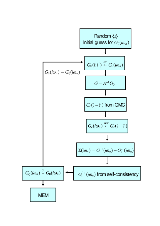
Figure 2: Sketch of the CDMFT algorithm using QMC method.

(1) We start by generating a random Ising spin configuration and an initial guess for the dynamical Weiss field $G_{0,\sigma}(\mu\mu^{\prime},i\omega_{n})$. The latter is usually taken as the non-interacting value.
(2) The Weiss field is Fourier transformed (FT) to obtain $G_{0,\sigma}(\mu\mu^{\prime},ll^{\prime})$.
(3) The propagator $G_{\sigma,\{s\}}(\mu\mu^{\prime},ll^{\prime})$ for the Ising spin configuration with $s_{\mu l}=\pm 1$ is calculated by explicit inversion of the matrix $A$ in Eq. 9 with $G$ replaced by $G_{0}$ in the latter equation.
(4) From then on, configurations are visited using single spin flips. When the change is accepted, the propagator is updated using Eq. 15.
(5) The physical cluster Green’s function $G_{c,\sigma}(\mu\mu^{\prime},l-l^{\prime})$ is determined as averages of the configuration-dependent propagator $G_{\sigma,\{s\}}(\mu\mu^{\prime},ll^{\prime}).$ The biased sampling guarantees that the Ising spin configurations are weighted according to Eq. 10.
(6) $G_{c,\sigma}(\mu\mu^{\prime},l-l^{\prime})$ is inverse Fourier transformed (IFT) by using a spline interpolation scheme (described in the previous section) to obtain $G_{c,\sigma}(\mu\mu^{\prime},i\omega_{n})$.
(7) The cluster self-energy $\Sigma(\mu\mu^{\prime},i\omega_{n})$ is computed from the cluster Green’s function using Eq. 2.
(8) A new dynamical Weiss field $G_{0,\sigma}^{\prime}(\mu\mu^{\prime},i\omega_{n})$ is calculated using the self-consistency condition Eq. 3.
(9) We go through the self-consistency loop (2)-(8) until the old and new Weiss fields converge within desired accuracy. Usually in less than 10 iterations the accuracy reaches a plateau (for example, relative mean-square deviation of $10^{-4}$ for $U=8,$ $\beta=5,$ or smaller for smaller interaction strength).
(10) After convergence is reached, the numerical analytical continuation is performed with MEM on the data from the binned measurements.
Figure 2 is a sketch of the CDMFT algorithm using the QMC method.

Figure 3: Speedup versus the number of nodes using MPI. Circles and diamonds represent speedup for the combined total number of measurements respectively equal to 64,000 and 32,000.

Fig. 3 shows the speedup achieved by parallelizing the code on the Beowulf cluster with the Message Passing Interface (MPI) MPI . The simplest way of parallelizing a QMC code is to make smaller number of measurements on each node and to average the results of each node to obtain the final result effectively with the desired number of measurements. In the CDMFT+QMC algorithm, this means that the heavy exchange of information between processors occurs at step (5) above. In Fig. 3 the combined total number of measurements is 64,000 for the circles, which means 2,000 measurements on each node for calculations with 32 nodes. The switch is at 10 Gb/s on infiniband and the processors are 3.6 GHz dual core Xeon. For a small number of nodes the speedup appears nearly perfect. As the number of nodes increases, it starts to deviate from the perfect line because the unparallelized part of the code starts to compensate the speedup. Speedup with less number of measurements on each node (diamonds) deviates further from the dashed line. Most of the calculations in the present work were done with 16 or 32 nodes and with up to 128,000 measurements.

V Comparison with Exact Results (Benchmarking)

The one-dimensional Hubbard model represents an ideal benchmark for the current and other cluster methods for several reasons. First, there exist several (analytically and numerically) exact results to compare with. Second, as mentioned before, the CDMFT scheme is expected to be in the worst case scenario in one-dimension, so that if it reproduces those exact results it is likely to capture the physics more accurately in higher dimensions. Third, a study of a systematic size dependence is much easier because of the linear geometry.

Figure 4: Density $n$ as a function of the chemical potential $\mu$ in the one-dimensional Hubbard model for $U/t=4$, $\beta=40$, $N_{c}=2$ (circles). The diamonds are obtained within the single site DMFT with the same parameters, while the solid curve is computed by the Bethe ansatz at zero temperature.

In Fig. 4 we show the density $n$ as a function of the chemical potential $\mu$ in the one-dimensional Hubbard model for $U/t=4$. It shows that CDMFT on the smallest cluster ($N_{c}=2$) already captures with high accuracy the evolution of the density as a function of the chemical potential and the compressibility divergence at the Mott transition Comment:1D , in good agreement with the exact Bethe ansatz result (solid curve) LW:1968 . This feature is apparently missed in the single site DMFT (diamonds) which also misses the Mott gap at half-filling for $U/t=4$. The deviation from the exact location where the density suddenly drops seems to be caused by a finite-size effect since we have checked that it does not come from finite temperature or from the imaginary-time discretization. The compressibility divergence as well as the Mott gap at half-filling for $U/t=4$ were recently reproduced by Capone et al. CCKCK:2004 using ED technique at zero temperature.

Figure 5: (a) Imaginary part of the local Green’s function $G_{11}$ and (b) real part of the nearest neighbor Green’s function $G_{12}$ in the one-dimensional Hubbard model for $U/t=7$, $n=1$ and $\beta=40$ on $N_{c}=2$ cluster. The dashed curves are DMRG results.

In Fig. 5 the imaginary part of the local Green’s function $G_{11}$ and the real part of the nearest-neighbor Green function $G_{12}$ are compared on the Matsubara axis with DMRG results shown as dashed curves. CDMFT with $N_{c}=2$ closely follows the DMRG on the whole Matsubara axis, and the two results become even closer for $N_{c}=4$ (not shown here). These results present an independent confirmation of the ability of CDMFT to reproduce the exact results in one-dimension with small clusters. This is very encouraging, since mean field methods are expected to perform even better as the dimensionality increases. In the application section on the Luttinger liquid, we will study quantities that are more sensitive to the size dependence.

VI Convergence with system size

VI.1 One-dimensional Hubbard Model

Figure 6: (a) Local Green’s function $G_{local}(\tau=\beta/2)$ and (b) nearest neighbor Green’s function $G_{near}(\tau=0)$ as a function of distance from the boundary of a linear chain with $N_{c}=24$ in the one-dimensional Hubbard model for $U/t=4$, $n=1$, $\beta=5$ (circles). The dashed curve is the exponential fit.

Fig. 6 shows the local Green function $G_{local}(\tau=\beta/2)$ and the nearest-neighbor Green function $G_{near}(\tau=0)$ as a function of distance from the boundary of a long linear chain ($N_{c}=24$). The local and nearest-neighbor Green functions rapidly (exponentially) approach the infinite cluster limit a few lattice sites away from the boundary. The largest deviation from the infinite cluster limit occurs essentially at the boundary. This feature has lead to recent attempts PK:2005 to greatly improve the convergence properties of CDMFT at large clusters by weighting more near the center of the cluster. It is called weighted-CDMFT, an approach which is being developed at present PK:2005 . In this paper we focus on small clusters and calculate lattice quantities without weighting (Eq. 4) and study how much correlation effect is captured by small clusters compared with the infinite size cluster. Because most of the detailed study of the Hubbard model MJPH:2004 ; CCKPK:2005 ; KKSTCK:2005 in the physically relevant regime (intermediate to strong coupling and low temperature) have been obtained only on small clusters, the present study will show how much those results represent the infinite cluster limit.

Figure 7(a) shows the imaginary-time Green function $G(\vec{k},\tau)$ at the Fermi point ($\vec{k}=\pi/2$) for $U/t=2$, $\beta=5$, $n=1$ with $N_{c}=2,4,8,12$. As the cluster size increases, $G(\vec{k},\tau)$ becomes smaller in magnitude and the infinite cluster limit is approached in a way opposite to that in finite size simulations, a phenomenon that was observed before in the Dynamical Cluster Approximation (DCA) MHJ:2000 .

Figure 7: (a) Imaginary-time Green’s function $G(\vec{k},\tau)$ at the Fermi point ($\vec{k}=\pi/2$) in the one-dimensional Hubbard model for $U/t=2$, $\beta=5$, $n=1$ with $N_{c}=2,4,8,12$ (solid, dotted, dashed, long-dashed curves). (b) Cluster size ($N_{c}=L$) dependence of $G(\vec{k},\beta/2)$ at small clusters. (c) The corresponding spectral function $A(\vec{k},\omega)$. The star in (b) represents the infinite cluster limit extracted from large clusters.

The quantity $G(\vec{k},\beta/2)$ at the Fermi wave vector is a useful measure of the strength of correlations. It varies from $-1/2$ for $U=0$ to $0$ for $U=\infty$ at half-filling. Thus throughout the paper $\left(U\neq 0\right)$ the “correlation ratio”

$$C_{r}\equiv\left[\frac{G(\vec{k},\beta/2)|_{N_{c}}+1/2}{G(\vec{k},\beta/2)|_{N_{c}=\infty}+1/2}\right]$$ (18)

will be used as an approximate estimate of how much the correlation effects are captured by a given cluster of size $N_{c}$, compared with the infinite cluster. $C_{r}$ is equal to unity when finite-size effects are absent.

Figure 7(b) shows the cluster size ($N_{c}=L$) dependence of $G(\vec{k},\beta/2)$ for small clusters. At small $L$ the curvature is upward so that $G(\vec{k},\beta/2)$ is much closer to the value of the infinite size cluster than what would be naively extrapolated from large clusters. The corresponding spectral function $A(\vec{k},\omega)$ in Fig. 7(c) shows a peak at the Fermi level for all clusters up to $L=12$. Although this looks like a quasiparticle peak, it is disproved by a close inspection of the corresponding self-energy.

We extract the self-energy from the lattice spectral function $A(\vec{k},\omega)$, and the relation between $A(\vec{k},\omega)$ and $G(\vec{k},\omega)$

$$G(\vec{k},\omega) = \int d\omega^{\prime}\frac{A(\vec{k},\omega^{\prime})}{\omega+i\delta-\omega^{\prime}}\;,$$

$$G(\vec{k},\omega) = \frac{1}{\omega+i\delta-\varepsilon_{\vec{k}}-\Sigma(\vec{k},\omega)}\;,$$ (19)

where $\delta$ is an infinitesimally small positive number and $\varepsilon_{\vec{k}}$ is the non-interacting energy dispersion.

Figure 8: Real (a) and imaginary (b) part of the self-energy $\Sigma(\vec{k},\omega)$ at the Fermi point ($\vec{k}=\pi/2$) in the one-dimensional Hubbard model for $U/t=2$, $\beta=5$, $n=1$ with $N_{c}=2,4,8,12$ (solid, dotted, dashed, long-dashed curves).

In spite of the peak in $A(\vec{k},\omega)$, the corresponding self-energy in Fig. 8 shows not only a local maximum at $\omega=0$ in the absolute value of the imaginary part, but also a positive slope at the Fermi level in the real part, which cannot be reconciled with a Fermi liquid. The scattering rate increases with increasing cluster size, as found in DCA MHJ:2000 , in contrast to the results of finite size simulations.

For the more correlated case of $U/t=4$ ($U$ equal to the bandwidth in one-dimension) in Fig. 9, $G(\vec{k},\tau)$ becomes much smaller in magnitude than $1/2$, the result for an uncorrelated system. A similar cluster size dependence is also found here. In Fig. 9(b) we compare our cluster size dependence with that of DCA MHJ:2000 (filled diamonds) for small clusters. Generally the curvatures are opposite, namely, upward in CDMFT and downward in DCA. This upward curvature enables even an $L=2$ cluster to capture, as measured by $C_{r}$, about $82\%$ of the correlation effect of the infinite size cluster. The corresponding spectral function $A(\vec{k},\omega)$ already shows a pseudogap for $L=2$, in contrast to the DCA result MHJ:2000 in which a pseudogap begins to appear for $L=8$.

Figure 9: (a) Imaginary-time Green’s function $G(\vec{k},\tau)$ at the Fermi point ($\vec{k}=\pi/2$) in the one-dimensional Hubbard model for $U/t=4$, $\beta=5$, $n=1$ with $N_{c}=2,4,8,12$ (solid, dotted, dashed, long-dashed curves). (b) Cluster size ($N_{c}=L$) dependence of $G(\vec{k},\beta/2)$ at small clusters. The filled diamonds are DCA results in Ref. MHJ:2000 with the same parameters. (c) The corresponding spectral function $A(\vec{k},\omega)$. The star in (b) represents the infinite cluster limit extracted from large clusters.

For $U/t=4$ the scattering rate in Fig. 10 is large enough to create the pseudogap in $A(\vec{k},\omega)$ for all clusters.

Figure 10: Real (a) and imaginary (b) part of the self-energy $\Sigma(\vec{k},\omega)$ at the Fermi point ($\vec{k}=\pi/2$) in the one-dimensional Hubbard model for $U/t=4$, $\beta=5$, $n=1$ with $N_{c}=2,4,8,12$ (solid, dotted, dashed, long-dashed curves).

For an even more correlated case of $U/t=6$ in Fig. 11, an $L=2$ cluster captures $99\%$ of the correlation effect (as measured by Eq. 18) of the infinite size cluster. Thus, at intermediate to strong coupling, short-range correlation effect (on a small cluster) starts to dominate the physics in the single particle spectral function, reinforcing our recent results KKSTCK:2005 based on the two-dimensional Hubbard model. The corresponding $A(\vec{k},\omega)$ shows a large pseudogap (or real gap) for all cluster sizes.

Figure 11: (a) Imaginary-time Green’s function $G(\vec{k},\tau)$ at the Fermi point ($\vec{k}=\pi/2$) in the one-dimensional Hubbard model for $U/t=6$, $\beta=5$, $n=1$ with $N_{c}=2,4,8,12$ (solid, dotted, dashed, long-dashed curves). (b) Cluster size ($N_{c}=L$) dependence of $G(\vec{k},\beta/2)$ for small clusters. (c) The corresponding spectral function $A(\vec{k},\omega)$. The star in (b) represents the infinite cluster limit extracted from large clusters.

The huge scattering rate in Fig. 12 at the Fermi energy is responsible for the large pseudogap (or real gap) in the spectral function.

Figure 12: Real (a) and imaginary (b) part of the self-energy $\Sigma(\vec{k},\omega)$ at the Fermi point ($\vec{k}=\pi/2$) in the one-dimensional Hubbard model for $U/t=6$, $\beta=5$, $n=1$ with $N_{c}=2,4,8,12$ (solid, dotted, dashed, long-dashed curves).

Recently there has been a debate about the convergence of the two quantum cluster methods (CDMFT and DCA) BK:2002 ; MJ:2002 ; AMJ:2005 using a highly simplified one-dimensional large-N model Hamiltonian where dynamics are completely suppressed in the limit of $N\rightarrow\infty$. The general consensus about the convergence of CDMFT (based on the study of this model Hamiltonian) is that purely local quantities defined on central cluster sites converge exponentially, while lattice quantities such as the lattice Green function converge with corrections of order $1/L$. Here we address this issue with a more realistic Hamiltonian, the one-dimensional Hubbard model at intermediate coupling of $U/t=4$. Figure 13(a) shows the cluster size dependence of the imaginary-time density of states $N(\tau)$ at $\tau=\beta/2$. We obtained $N(\tau)$ in two different ways: Taking the average of the lattice Green function (obtained without weighting) over the Brillouin zone (circles) and taking the local Green function at the center of the cluster (diamonds). For $N_{c}=2$ they are identical while for larger clusters, $N(\beta/2)$ obtained from the local Green’s function approaches the $N_{c}=\infty$ limit much faster than that from the lattice Green function that converges linearly in $1/L$ Comment:Weighting , in agreement with the previous results based on the large-N model. In spite of this slow convergence, the slope is so small that the $N_{c}=2$ cluster already accounts for $95\%$ of the correlation effect of the infinite cluster (using $C_{r}$ as a measure with $G(\vec{k},\beta/2)\rightarrow N(\beta/2)$), much larger than $82\%$ for $G(\vec{k},\beta/2)$. Figure 13(b) is a close up of Fig. 13(a) at large $L$. $N(\beta/2)$ from the two methods converge to a single value as $L\rightarrow\infty$. $N(\beta/2)$ from the local Green function approaches the infinite-size limit much faster than $1/L^{2}$ and apparently converges exponentially.

Figure 13: (a) Cluster size ($N_{c}=L$) dependence of the imaginary-time density of states $N(\tau)$ at $\tau=\beta/2$ in the one-dimensional Hubbard model for $U/t=4$, $\beta=5$, $n=1$. The circles are obtained from the average of the lattice Green’s function (without weighting) over the Brillouin zone, while the diamonds are calculated from the local Green’s function at the center of the cluster (a linear chain in one-dimension). (b) Close up of the region at large $L$. The star in (b) represents the infinite cluster limit extracted by a linear extrapolation at large clusters.

VI.2 Two-dimensional Hubbard Model

The two-dimensional Hubbard Hamiltonian on a square lattice has been intensively studied for many years, especially since Anderson’s seminal paper Anderson:1987 on high temperature superconductivity. There is mounting evidence that this model correctly describes the low-energy physics of the copper oxides TKS:2005 . In addition to various types of long-range order observed in the cuprates, one must understand the intriguing normal state pseudogap TS:1999 in the underdoped regime. In this section we focus on the size dependence of the spectral function for the half-filled two-dimensional Hubbard model for small clusters at finite temperature. Figure 14(a) shows the imaginary-time Green’s function $G(\vec{k},\tau)$ at the Fermi surface ($\vec{k}=(\pi,0)$) for $U/t=4.4$, $\beta=4$, $n=1$ with $N_{c}=2\times 2,3\times 3,4\times 4,6\times 6$ Comment:2D . As the cluster size increases, $G(\vec{k},\tau)$ decreases in magnitude, as in the one-dimensional case, a behavior opposite to that of finite size simulations. This trend is in agreement with DCA JMHM:2001 , as shown in Figure 14(b). The spectral weight $A(\vec{k},\omega)$ for the same parameters shows a peak at $\omega=0$ for small $L$ ($N_{c}=L\times L$) but starts exhibiting a pseudogap for $L\geq 6$. This is consistent with our recent results with CDMFT+ED KKSTCK:2005 where we find that at weak coupling a large correlation length (on a large cluster) is required to create a pseudogap. From the Two-Particle Self-Consistent (TPSC) approach, we know that to obtain a pseudogap in this regime of coupling strength, the antiferromagnetic correlation length has to be larger than the single-particle thermal de Broglie wave length Vilk:1997 ; Vilk:1996 .

Figure 14: (a) Imaginary-time Green’s function $G(\vec{k},\tau)$ at the Fermi surface ($\vec{k}=(\pi,0)$) in the two-dimensional Hubbard model for $U/t=4.4$, $\beta=4$, $n=1$ with $N_{c}=2\times 2,3\times 3,4\times 4,6\times 6$ (solid, dotted, dashed, long-dashed curves). $\Delta\tau=0.25$ is used here. (b) Cluster size ($N_{c}=L\times L$) dependence of $G(\vec{k},\beta/2)$ at small clusters. The filled diamonds are DCA results of Ref.JMHM:2001 . (c) The corresponding spectral function $A(\vec{k},\omega)$. The star in (b) represents the infinite cluster limit extracted by a linear extrapolation at large clusters.

Unlike in the one-dimensional case, the imaginary part of the self-energy for $L\leq 4$ has a very shallow maximum or a minimum at the Fermi level, accompanied by a negative slope in the real part as seen in Fig. 15. This feature is consistent with a Fermi liquid at finite temperature. For $L\geq 6$, however, the scattering rate has a local maximum together with a large positive slope in the real part, resulting in the pseudogap in the spectral function.

Figure 15: Real (a) and imaginary (b) part of the self-energy $\Sigma(\vec{k},\omega)$ at the Fermi surface ($\vec{k}=(\pi,0)$) in the two-dimensional Hubbard model for $U/t=4.4$, $\beta=4$, $n=1$ with $N_{c}=2\times 2,3\times 3,4\times 4,6\times 6$ (solid, dotted, dashed, long-dashed curves).

Next we study the more correlated case of $U/t=8$ in Fig. 16. This regime is believed to be relevant for the hole-doped cuprates. When $U$ becomes equal to the bandwidth, the cluster size dependence of $G(\vec{k},\tau)$ is extremely weak. As can be seen in Fig. 16(b), $N_{c}=2\times 2$ already accounts for more than $95\%$ of the correlation effect (as measured by Eq. 18) of the infinite size cluster in the single particle spectrum, supporting our recent result obtained with CDMFT+ED method KKSTCK:2005 in the two-dimensional Hubbard model. The large gap in $A(\vec{k},\omega)$ does not change significantly with increasing cluster size.

Figure 16: (a) Imaginary-time Green’s function $G(\vec{k},\tau)$ at the Fermi surface ($\vec{k}=(\pi,0)$) in the two-dimensional Hubbard model for $U/t=8$, $\beta=5$, $n=1$ with $N_{c}=2\times 2,3\times 3,4\times 4$ (solid, dotted, dashed curves). (b) Cluster size ($N_{c}=L\times L$) dependence of $G(\vec{k},\beta/2)$ for small clusters. (c) The corresponding spectral function $A(\vec{k},\omega)$. The star in (b) represents the infinite cluster limit extracted by a linear extrapolation.

The self-energy for $U/t=8$ (Fig. 17) appears similar to what was found in the one-dimensional case with $U/t=6$ where the imaginary part has a very large peak at the Fermi energy, leading to what appears as a large gap in $A(\vec{k},\omega)$.

Figure 17: Real (a) and imaginary (b) part of the self-energy $\Sigma(\vec{k},\omega)$ at the Fermi surface ($\vec{k}=(\pi,0)$) for the two-dimensional Hubbard model with $U/t=8$, $\beta=5$, $n=1$ for $N_{c}=2\times 2,3\times 3,4\times 4$ (solid, dotted, dashed curves).

When short-range spatial correlations are treated explicitly, the well-known metal-insulator transition in the single site DMFT disappears immediately as shown in our recent articles KKSTCK:2005 ; KGT:2005 . Frustration would restore the metal-insulator transition PBK:2004 .

VII Spinons and holons in CDMFT

Spinon and holon dispersions were recently found experimentally in a quasi-one-dimensional organic conductors away from half-filling by Claessen et al. CSSBDJ:2002 . These separate features of the dispersion in a Luttinger liquid are a challenge for numerical approaches. Indeed, we know from bosonization and from the renormalization group Voit:1995 that they arise from long-wavelength physics, hence it is is not obvious how these features can come out from small cluster calculations. They have been seen theoretically in the one-dimensional Hubbard model away from half-filling by Benthien et al. BGJ:2004 using Density-Matrix Renormalization Group. The evidence from straight QMC calculations is based on the analysis of chains of size 64 ZAHS:1998 . On the other hand, with Cluster Perturbation Theory one finds clear signs of the holon and spinon dispersion at zero temperature already for clusters of size 12 SPP:2000 .

As an application of CDMFT+QMC, we present in this section a study of the appearance of spinon and holons as a function of system size at finite temperature. The spectral function $A(\vec{k},\omega)$ and its dispersion curve are calculated in the one-dimensional Hubbard model for $U/t=4$, $\beta=5$, $n=0.89$ with several sizes of cluster (obtained without weighting) shown in Fig. 18 to demonstrate the ability of CDMFT to reproduce highly nontrivial physics in one-dimensional systems. For $N_{c}=2,$ $A(\vec{k},\omega)$ has only one broad feature near $\vec{k}=0$ and $\pi$, while for $N_{c}=12$ it starts showing, near $\vec{k}=\pi$, continuous spectra that are bounded by two sharp features. Near $\vec{k}=0$ the two features do not show up clearly. For $N_{c}=24$ however, the spectral function shows the separation of spinon and holon dispersions near both $\vec{k}=0$ and $\pi$, even if the temperature $\beta=5$ is relatively large. These features are in agreement with recent QMC calculations for the one-dimensional Hubbard model Matsueda:2005 ; Abendschein:2006 . As $\vec{k}$ approaches $\vec{k}_{F}$, we loose the resolution necessary to separate the two spectra. For $U/t=6$ we obtain a similar result, while at weak coupling ($U/t=2$) we do not resolve the separation up to $L=24$.

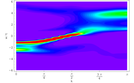
Figure 18: Spectral function $A(\vec{k},\omega)$ for (a) $N_{c}=2$, (b) $N_{c}=12$, (c) $N_{c}=24$, and dispersion curve (bottom) for $N_{c}=24$ in the one-dimensional Hubbard model for $U/t=4$, $\beta=5$, $n=0.89$.

VIII Summary, conclusions and outlook

To summarize, we have studied the Hubbard model as an example of strongly correlated electron systems using the Cellular Dynamical Mean-Field Theory (CDMFT) with quantum Monte Carlo (QMC) simulations. The cluster problem may be solved by a variety of techniques such as exact diagonalization (ED) and QMC simulations. We have presented the algorithmic details of CDMFT with the Hirsch-Fye QMC method for the solution of the self-consistently embedded quantum cluster problem. We have used the one-dimensional half-filled Hubbard model to benchmark the performance of CDMFT+QMC particularly for small clusters by comparing with the exact results. We have also calculated the single-particle Green’s functions and self-energies on small clusters to study the size dependence of the results in one- and two-dimensions, and finally, we have shown that spin-charge separation in one dimension can be studied with this approach using reasonable cluster sizes.

To be more specific, it has been shown that in one dimension, CDMFT+QMC with two sites in the cluster is already able to describe with high accuracy the evolution of the density as a function of chemical potential and the compressibility divergence at the Mott transition, in good agreement with the exact Bethe ansatz result. This presents an independent confirmation of the ability of CDMFT to reproduce the compressibility divergence with small clusters. In the previous tests with CDMFT+ED, some sensitivity to the so-called distance function, had been noticed CCKCK:2004 . This question does not arise with QMC. This is very encouraging, since mean field methods would be expected to perform even better as the dimensionality increases. We also looked at the cluster size dependence of the Green’s function $G(\vec{k},\tau).$ It becomes smaller in magnitude with increasing system size and the infinite cluster limit is approached in the opposite way to that in finite size simulations, as was observed before in another quantum cluster scheme (DCA) MHJ:2000 . With increasing $U$ the result on the smallest cluster rapidly approaches that of the infinite size cluster. Large scattering rate and a positive slope in the real part of the self-energy in one-dimension suggest that the system is a non-Fermi liquid for all the parameters studied here.

In two-dimensions, a similar size dependence to the one-dimensional case is found. At weak coupling a pseudogap appears only for large clusters in agreement with the expectation that at weak coupling a large correlation length (on a large cluster) is required to create a gap. At intermediate to strong coupling, even the smallest cluster ($N_{c}=2\times 2$) accounts for more than $95\%$ of the correlation effect in the single particle spectrum of the infinite size cluster, (as measured by Eq.(18)). This is consistent with our earlier study that showed indirectly that for $U$ equal to the bandwidth or larger, short-range correlation effect (available in a small cluster) starts to dominate the physics KKSTCK:2005 . This presents great promise that some of the important problems in strongly correlated electron systems may be studied highly accurately with a reasonable computational effort.

Finally, we have shown that CDMFT+QMC can describe highly nontrivial long wavelength Luttinger liquid physics in one-dimension. More specifically, for $U=4$ and $\beta=5$ the separation of spinon and holon dispersions is clear even for $N_{c}=24.$

Issues that can now be addressed in future work include that of the origin of the pseudogap observed in hole-underdoped cuprates. Since the parent compounds of the cuprates are Mott-Hubbard insulators, an understanding of such an insulator and its evolution into a correlated metal upon doping is crucial. In particular, CDMFT+QMC offers the possibility of calculating the pseudogap temperature to compare with experiment. This has been successfully done at intermediate coupling with TPSC TKS:2005 , but at strong coupling, quantum cluster approaches are needed. Single-site DMFT is not enough since, for example, high resolution QMC study for the half-filled 2D Hubbard model MHSD:1995 ; PLH:1995 found two additional bands besides the familiar Hubbard bands in the spectral function. These are apparently caused by short-range spatial correlations that are missed in the single-site DMFT. The search for a coherent understanding of the evolution of a Mott insulator into a correlated metal by doping at finite temperature has been hampered by the severe minus problem in QMC away from half-filling and at low temperature. An accurate description of the physics at intermediate to strong coupling with CDMFT+QMC with small clusters (as shown in this paper) and modest sign problems in quantum cluster methods (as shown in DCA JMHM:2001 ) give us the tools to look for a systematic physical picture of the finite temperature pseudogap phenomenon at strong coupling.

Another issue that can be addressed with CDMFT+QMC is that of the temperature range over which spin-charge separation occurs in the one-dimensional Hubbard model. In other words, at what temperature does Luttinger Physics breaks down as a function of $U$, and when it breaks down what is the resulting state? We saw in this paper that even a single peak in the single-particle spectral weight does not immediately indicate a Fermi liquid.

Finally, one methodological issue. Two-particle correlation functions are necessary to identify second order phase transitions by studying the divergence of the corresponding susceptibilities. This can be done with DCA MJPH:2004 . In the present paper, instead, we focused on one-particle quantities such as the Green’s function and related quantities. In some sense, quantum cluster methods such as CDMFT use irreducible quantities (self-energy for one-particle functions and irreducible vertices for two-particle functions) of the cluster to compute the corresponding lattice quantities. Since the CDMFT is formulated entirely in real space and the translational symmetry is broken at the cluster level, it appears extremely difficult, in practice, to obtain two-particle correlation functions and their corresponding irreducible vertex functions in a closed form like matrix equations to look for instabilities. One way to get around this problem is, as in DMFT, to introduce mean-field order parameters such as antiferromagnetic and $d-wave$ superconducting orders, and to study if they are stabilized or not for given parameters such as temperature and doping level. In this way one can, for example, construct a complete phase diagram of the Hubbard model, including a possible regime in which several phases coexist. Zero-temperature studies with CDMFT+ED KCCKSKT:2005 and with the Variational Cluster Approximation SLMT:2005 ; HAAP:2005 have already been performed along these lines.

- (1) E. Dagotto, Rev. Mod. Phys. 66, 763 (1994).
- (2) M. H. Hettler, A. N. Tahvildar-Zadeh, M. Jarrell, T. Pruschke, and H. R. Krishnamurthy, Phys. Rev. B 58, R7475 (1998).
- (3) D. Sénéchal, D. Perez, and M. Pioro-Ladrière, Phys. Rev. Lett. 84, 522 (2000).
- (4) A. I. Lichtenstein and M. I. Katsnelson, Phys. Rev. B 62, R9283 (2000).
- (5) G. Kotliar, S. Savrasov, G. Pallson, and G. Biroli, Phys. Rev. Lett. 87, 186401 (2001).
- (6) M. Potthoff, Eur. Phys. J. B 32, 429 (2003); Phys. Rev. Lett. 91, 206402 (2003).
- (7) T. Maier, M. Jarrell, T. Pruschke, and M. H. Hettler, Rev. Mod. Phys. 77, 1027 (2005) .
- (8) A. Georges and G. Kotliar, Phys. Rev. B 45, 6479 (1992).
- (9) M. Jarrell, Phys. Rev. Lett. 69, 168 (1992).
- (10) A. Georges, G. Kotliar, W. Krauth, and M. J. Rozenberg, Rev. Mod. Phys. 68, 13 (1996).
- (11) T. Timusk and B. Statt, Rep. Prog. Phys. 62, 61 (1999); M. R. Norman, D. Pines and C. Kallin, Adv. Phys. 54, 715 (2005).
- (12) O. Parcollet, G. Biroli, and G. Kotliar, Phys. Rev. Lett. 92, 226402 (2004).
- (13) J. Hirsch and R. Fye, Phys. Rev. Lett. 56, 2521 (1986).
- (14) S. S. Kancharla, M. Civelli, M. Capone, B. Kyung, D. Sénéchal, G. Kotliar, A.-M.S. Tremblay, cond-mat/0508205.
- (15) C. Bolech, S. S. Kancharla, and G. Kotliar, Phys. Rev. B 67, 075110 (2003).
- (16) M. Capone, M. Civelli, S. S. Kancharla, C. Castellani, and G. Kotliar, Phys. Rev. B 69, 195105 (2004).
- (17) B. Kyung, S. S. Kancharla, D. Sénéchal, A. -M. S. Tremblay, M. Civelli, and G. Kotliar, Phys. Rev. B 73, 165114 (2006).
- (18) Tudor D. Stanescu and Gabriel Kotliar, cond-mat/0508302.
- (19) R.R. dos Santos, Brazilian Journal of Physics 33 36 (2003).
- (20) J. Hirsch, Phys. Rev. B 28, 4059 (1983).
- (21) (not ) is required in order to reproduce the correct fermionic Green’s function from the determinant of . The antiperiodicity comes from the antiperiodic boundary condition of the fermionic Green’s function under a shift of . See R. Blankenbecler, D. J. Scalapino, and R. L. Sugar, Phys. Rev. D 24, 2278 (1981) and Hirsch:1983 .
- (22) M. Jarrell and J. Gubernatis, Physics Reports 269, 133 (1996).
- (23) S. Allen, private communications.
- (24) V. S. Oudovenko and G. Kotliar, Phys. Rev. B 65, 075102 (2002).
- (25) M. Jarrell, T. Maier, C. Huscroft, and S. Moukouri, Phys. Rev. B 64, 195130 (2001).
- (26) G. Kotliar, S. Y. Savrasov, K. Haule, V. S. Oudovenko, O. Parcollet, and C.A. Marianetti, cond-mat/0511085.
- (27) W. Gropp, E. Lusk, and A. Skjellum, 1999, Using MPI: Portable Parallel Programming with the Message Passing Interface, 2nd ed. (The MIT Press).
- (28) For the kink near is rounded.
- (29) E. H. Lieb and F. Y. Wu, Phys. Rev. Lett. 20, 1445 (1968).
- (30) O. Parcollet and G. Kotliar, unpublished.
- (31) M. Civelli, M. Capone, S. S. Kancharla, O. Parcollet, and G. Kotliar, Phys. Rev. Lett. 95, 106402 (2005).
- (32) S. Moukouri, C. Huscroft, and M. Jarrell, cond-mat/0004279.
- (33) G. Biroli and G. Kotliar, Phys. Rev. B 65, 155112 (2002).
- (34) T. Maier and M. Jarrell, Phys. Rev. B 65, 041104(R) (2002).
- (35) K. Aryanpour, T. Maier, and M. Jarrell, Phys. Rev. B 71, 037101 (2005).
- (36) We believe that with appropriate weighting the convergence can be much faster than linear in at large clusters.
- (37) P. W. Anderson, Science 235, 1196 (1987).
- (38) A. -M. S. Tremblay, B. Kyung, and D. Sénéchal, Fizika Nizkikh Temperatur (Low Temperature Physics), 32, 561 (2006).
- (39) Because open boundary conditions are imposed in the cluster, an odd number of linear size such as 3 and 5 can be used without causing any irregularity. Although an open cluster breaks the full lattice translational symmetry at the cluster level (which is eventually restored by Eq. 4), here it works to our advantage.
- (40) Y. Vilk and A.-M. Tremblay, J. Phys I (France) 7, 1309 (1997).
- (41) Y. Vilk and A.-M. Tremblay, Europhys. Lett. 33, 159 (1996).
- (42) B. Kyung, A. Georges, and A. -M. S. Tremblay, cond-mat/0508645.
- (43) R. Claessen, M. Sing, U. Schwingenschloegl, P. Blaha, M. Dressel, and C.S. Jacobsen, Phys. Rev. Lett. 88, 096402 (2002).
- (44) For a review, see J. Voit, Rep. Prog. Phys. 58, 977 (1995).
- (45) H. Benthien, F. Gebhard, and E. Jeckelmann, Phys. Rev. Lett. 92, 256401 (2004).
- (46) M. G. Zacher, E. Arrigoni, W. Hanke, and J. R. Schrieffer, Phys. Rev. B 57, 6370 (1998).
- (47) H. Matsueda, N. Bulut, T. Tohyama, and S. Maekawa, Phys. Rev. B 72, 075136 (2005).
- (48) A. Abendschein and F. F. Assaad, cond-mat/0601222.
- (49) A. Moreo, S. Hass, A. W. Sandvik, and E. Dagotto, Phys. Rev. B 51, 12 045 (1995).
- (50) R. Preuss, W. von der Linden, and W. Hanke, Phys. Rev. Lett. 75, 1344 (1995).
- (51) D. Sénéchal, P.-L. Lavertu, M.-A. Marois and A.-M. S. Tremblay, Phys. Rev. Lett. 94, 156404 (2005).
- (52) W. Hanke, M. Aichhorn, E. Arrigoni and M. Potthoff, Correlated band structure and the ground-state phase diagram in high- cuprates (2005), eprint cond-mat/0506364.