Anomalous in-plane magneto-optical anisotropy of self-assembled quantum dots

Abstract

We report on a complex nontrivial behavior of the optical anisotropy of quantum dots that is induced by a magnetic field in the plane of the sample. We find that the optical axis either rotates in the opposite direction to that of the magnetic field or remains fixed to a given crystalline direction. A theoretical analysis based on the exciton pseudospin Hamiltonian unambiguously demonstrates that these effects are induced by isotropic and anisotropic contributions to the heavy-hole Zeeman term, respectively. The latter is shown to be compensated by a built-in uniaxial anisotropy in a magnetic field $B_{C}=0.4$ T, resulting in an optical response typical for symmetric quantum dots.

Self assembled semiconductor quantum dots (QDs) attract much fundamental and practical research interest. E.g., QD optical properties are exploited in low-threshold lasers, while QDs are also proposed as optically controlled qubits qubit ; Optic_qubit . An important, and frequently somewhat neglected aspect of QDs is the relationship between their symmetry and their optical properties. We recently showed that extreme anisotropy of QDs can lead to efficient optical polarization conversion Conversion .

Self assembled QDs grown by molecular beam epitaxy generally possess a well-defined ($z$) axis along the $\mathrm{[001]}$ growth direction which serves as the spin quantization axis. It thus makes sense to assume the dots have $D_{2d}$ point-group symmetry, and to describe of the influence of an external magnetic field using an isotropic transverse heavy-hole g-factor $g_{hh}^{\perp}$ in the plane of the sample ($xy$). Many actual QDs, however, exhibit an elongated shape in the plane and a similar strain profile, their symmetry is reduced to $C_{2v}$ or below. In this case the in-plane heavy hole g-factor is no longer isotropic ani_g . Moreover, even in zero field the degeneracy of the radiative doublet is lifted due to the anisotropic exchange splitting AlongatedShape ; AniSplit ; Book . Any of these issues will give rise to optical anisotropy, resulting in the linear polarization of the photoluminescence (PL).

In this manuscript, we discuss the optical anisotropy of QDs in the presence of a magnetic field. Classically, the polarization axis of the luminescence of a given sample should be collinear with the direction of the magnetic field. This so-called Voigt effect, implies that when rotating the sample over an angle $\alpha$ while keeping the direction of the magnetic field fixed, one observes a constant polarization (in direction and amplitude) for the luminescence. Mathematically one can express this behavior as following a zeroth order spherical harmonic dependence on $\alpha$. This situation changes drastically for low dimensional heterostructures because of the complicated valence band structure. Kusrayev et al. Ku_Ku observed a second spherical harmonic component (i.e., $\pi$-periodic oscillations under sample rotation) in the polarization of emission from narrow quantum wells (QWs). This result was explained in terms of a large in-plane anisotropy of the heavy-hole g-factor $g_{hh}^{xx}=-g_{hh}^{yy}$ . Subsequently, this interpretation was substantiated using a microscopic theory SemRya ; QD_dich .

Here, we report the observation of a fourth harmonic in the magneto-optical anisotropy (i.e. $\pi/2$-periodic oscillations in the polarization of the emitted light under sample rotation) from CdSe/ZnSe self assembled QDs. We demonstrate that this effect is quite general. An important consequence is that the polarization axis hardly follows the magnetic field direction, thus the classical Voigt effect is not observed for QD emission associated with the heavy-hole exciton. Moreover, in contrast to earlier studies of in-plane magneto-optical anisotropies, we consider the contributions of the electron-hole exchange interaction, which have been ignored for QWs Ku_Ku ; SemRya and are zero for charged QDs ani_g . An anisotropic exchange splitting may lead to the occurrence of a compensating magnetic field $B_{C}$. When the externally applied field equals $B_{C}$, the amplitude of the second harmonic crosses zero, resulting in a highly symmetrical optical response of extremely anisotropic QDs. For our QDs we find $B_{C}\approx 0.4$ T. Intriguingly, at this condition the polarization axis rotates away from the magnetic field direction.

In order to measure anisotropy we used the detection scheme presented in Fig. 1a. The direction of the in-plane magnetic field is fixed, while the sample is rotated over an angle $\alpha$. The degree of linear polarization is now defined as $\rho_{\gamma}(\alpha)=(I_{\gamma}-I_{\gamma+90^{\circ}})/(I_{\gamma}+I_{\gamma+90^{\circ}})$. Here the angle $\gamma$ corresponds to the orientation of the detection frame with respect to the magnetic field and $I_{\gamma}$ is the intensity of the PL polarized along the direction $\gamma$. Within an approximation of weak magnetic fields, a sample that has $C_{2v}$ point symmetry in general may have only three spherical harmonic components Ku_Ku linking the polarization of the emission to the sample rotation angle $\alpha$. Thus, one has for $\gamma=0^{\circ}$ and $\gamma=45^{\circ}$

$$\rho_{0}(\alpha)=a_{0}+a_{2}\,\cos 2\alpha+a_{4}\,\cos 4\alpha$$

$$\rho_{45}(\alpha)=a_{2}\,\sin 2\alpha+a_{4}\,\sin 4\alpha\,,$$ (1)

with $a_{0}$, $a_{2}$ and $a_{4}$ the amplitudes of the zeroth, second and fourth harmonic, respectively. $\alpha$ is measured with respect to the $\mathrm{[1\overline{1}0]}$ crystalline axis.

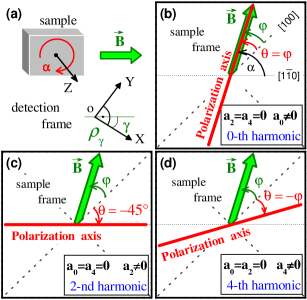
Figure 1: (Color online) (a) Schematic layout of the angle-resolved experiments where $\alpha$ is the rotation angle of the sample. The detection frame $\rho_{\gamma}$ is rotated by an angle $\gamma$ (equal to $0^{\circ}$ or $45^{\circ}$) with respect to the magnetic field $\mathbf{B}$. (b)-(d) Different scenarios for magneto-optical anisotropy (shown in the sample frame). (b) The polarization axis follows the magnetic field and $\theta=\varphi$, leading to a zeroth harmonic in the angle scan. (c) The polarization axis is fixed at $\theta=\mathrm{const}(\varphi)$, resulting in a second harmonic in the angle scan. (d) The polarization axis rotates away from the magnetic field with $\theta=-\varphi$, leading to a fourth harmonic in the angle scan.

For an analysis of the various orientation effects it is more convenient to turn from the detection frame to the sample frame. Now the sample orientation is fixed and the magnetic field rotates by the same angle $\alpha$ but in opposite direction (Figs. 1b-d). The orientation of the magnetic field in the spin Hamiltonian, which we discuss below, can be incorporated more conveniently using a basis along the $\mathrm{[100]}$, $\mathrm{[010]}$ and $\mathrm{[001]}$ crystalline axes. Therefore we introduce the angle $\varphi$ between the magnetic field direction and the $\mathrm{[100]}$ axis, as $\varphi\equiv\alpha-45^{\circ}$. We then consider the orientation of the polarization axis described by an angle $\theta$ in the same $\mathrm{[100]}$ basis.

We are now in a position to discuss some limiting cases of Eq. (1). When the zeroth order spherical harmonic dominates, $|a_{0}|\gg|a_{2}|,|a_{4}|$, the polarization axis of the emission coincides with the magnetic field direction for any orientation of the sample, $\theta(\varphi)=\varphi$ (Fig. 1b). For a dominantly second harmonic response, $|a_{2}|\gg|a_{0}|,|a_{4}|$, the polarization axis is fixed to a distinct sample direction and does not depend on the magnetic field orientation. In our experiments, the fixed polarization axis is $\mathrm{[1\overline{1}0]}$ and $\theta(\varphi)=-45^{\circ}$ (Fig. 1c). The most interesting behavior is observed for the fourth harmonic $|a_{4}|\gg|a_{0}|,|a_{2}|$, when the polarization $\rho_{\gamma}(\alpha)$ in the detection frame changes twice as fast as any polarization linked to the sample frame. This implies that the polarization axis turns in opposite direction to that of the magnetic field, and $\theta(\varphi)=-\varphi$ (Fig. 1d). In other words, it is collinear with the magnetic field when $\mathbf{B}\parallel\mathrm{[100]},\mathrm{[010]}$ and perpendicular to the magnetic field when $\mathbf{B}\parallel\mathrm{[110]},\mathrm{[1\overline{1}0]}$.

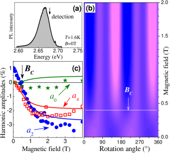
Figure 2: (Color online) (a) PL emission spectrum of the CdSe/ZnSe QD sample. (b) 3D plot of the linear polarization $\rho_{45}(\alpha,B)$ as function of the rotation angle $\alpha$ and magnetic inductance $B$. Light (red) and dark (blue) areas correspond to positive and negative values of $\rho_{45}(\alpha,B)$, respectively. (c) Amplitudes of the zeroth ($a_{0}$), second ($a_{2}$) and fourth ($a_{4}$) spherical harmonics vs $B$. The symbols are experimental data and the solid lines result from calculations. The arrows in panels (b) and (c) indicate the compensating field $B_{C}$ where the linear polarization is $\pi/2$-periodic ($a_{2}=0$).

We studied the magneto-optical anisotropy of CdSe QDs in a ZnSe host. The samples were fabricated on (001) GaAs substrates using molecular beam epitaxy and self-assembly after depositing one monolayer of CdSe on a 50 nm thick ZnSe layer. The QDs were then capped by 25 nm of ZnSe. For optical excitation at 2.76 eV we used a stilbene dye-laser pumped by the UV-lines of an Ar-ion laser. A typical PL spectrum is shown in Fig. 2a. For detection of the linear polarization we applied a standard technique using a photo-elastic modulator and a two-channel photon counter Conversion . The angle scans were performed with the samples mounted on a rotating holder controlled by a stepping motor with an accuracy better than $1^{\circ}$. Magnetic fields up to 4 T were applied in the sample plane (Voigt geometry), optical excitation was done using a depolarized laser beam. The degree of linear polarization of the luminescence of the QDs was determined at 2.68 eV at a temperature $T=1.6$ K.

The result of angle scans of $\rho_{45}$ for various magnetic field strengths is shown in Fig. 2b. In zero magnetic field the linear polarization is $\pi$-periodic (see also Fig. 3a). This demonstrates the low ($C_{2v}$) symmetry of the QDs (the dots are elongated in the plane) resulting in a finite value of $a_{2}$ in Eq. (1). One can regard this measurement as reflecting the ’built-in’ linear polarization of the array of dots. For high magnetic fields $a_{2}$ changes sign and an additional fourth harmonic signal appears (see also Fig. 3c). At an intermediate magnetic field $B_{C}\approx 0.4$ T the second harmonic crosses zero, while the fourth harmonic remains finite (see also Fig. 3b). The resulting $\pi/2$-periodic optical response corresponds to the higher ($D_{2d}$) symmetry expected for symmetric (i.e., not elongated) QDs. This observation clearly demonstrates that the in-plane optical anisotropy of QDs can be compensated by in-plane Zeeman terms. We also find that the zeroth harmonic signal is weak. This is clearly seen e.g. for the $\rho_{0}$ angle scan in Fig. 3d which was taken for $B=4$ T, where the field-induced alignment is saturated.

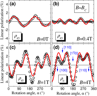
Figure 3: (Color online) Angle scans of the linear polarization of the luminescence. The symbols are experimental data, solid lines represent calculations based on the Hamiltonian of Eq. (7). (a) Built-in linear polarization ($B=0$ T). (b) A highly symmetrical optical response (i.e. $\pi/2$-periodic) appears at a compensating field $B_{c}\approx 0.4$ T. (c) Angle scan in a magnetic field $B=1$ T exeeding $B_{C}$. (d) Angle scan in the saturation regime, $B=4$ T. The detection frame $\rho_{\gamma}$ in (a)-(c) is rotated by an angle $\gamma=45^{\circ}$; in (d) $\gamma=0^{\circ}$. The arrows indicate the points where the orientation of the magnetic field aligns with high-symmetry directions in the sample frame.

We now model our observations using a pseudospin formalism SemRya ; LinPolDMS . We denote by $|+Sp\rangle$ and $|-Sp\rangle$ the wavefunctions of an electron ($p=el$) or heavy-hole ($p=hh$) with pseudospin projection $\pm S$ along the $z$ direction. We define a pseudospin Hamiltonian in matrix form for each band, as follows

$$\mathcal{H}_{p}=\frac{\delta_{p}}{2}(\sigma_{x}\cos\theta_{p}+\sigma_{y}\sin\theta_{p})\,,$$ (2)

where $\sigma_{x}$ and $\sigma_{y}$ are the Pauli matrices. This Hamiltonian has eigenfunctions $\Psi_{p}^{\pm 1}\propto|+Sp\rangle\pm e^{i\theta_{p}}|-Sp\rangle$. The optical matrix elements for a transition between electron and heavy-hole bands are $\langle\pm\frac{1}{2}el|\hat{P}|\pm\frac{3}{2}hh\rangle=\mp e_{\pm}$ Book , where $\hat{P}$ is the dipole momentum operator. We define $e_{\pm}=(e_{x}\pm ie_{y})/\sqrt{2}$ with $e_{x}\parallel[100]$ and $e_{y}\parallel[010]$ are unit vectors. We thus find for the optical matrix elements for the four possible optical transitions

$$\langle\Psi_{el}^{\eta}|\hat{P}|\Psi_{hh}^{\mu}\rangle\propto-e_{+}+\eta\mu\,e^{i(\theta_{hh}-\theta_{el})}e_{-}\,.$$ (3)

These matrix elements thus predict a linear polarization with an axis that is rotated over an angle $\theta=\frac{1}{2}(\theta_{hh}-\theta_{el})$ from [100] when $\eta=-\mu$ ($\eta,\mu=\pm 1$), and rotated over $\theta=\frac{1}{2}(\theta_{hh}-\theta_{el})+90^{\circ}$ when $\eta=\mu$.

For an electron in an external magnetic field $B$, we can write the Zeeman Hamiltonian as

$$\mathcal{H}_{el}=\frac{1}{2}g_{el}^{\bot}\mu_{B}\left(\sigma_{x}B\cos\varphi+\sigma_{y}B\sin\varphi\right)\,,$$ (4)

where $g_{el}^{\bot}$ is the electron g-factor, yielding directly $\theta_{el}=\varphi$. For $D_{2d}$ symmetry, the interaction of holes with an in-plane magnetic field $B$ can be described by HoleSplit

$$\mathcal{H}_{hh}=q_{1}\,g_{0}\mu_{B}\left(J_{x}^{3}B\cos\varphi+J_{y}^{3}B\sin\varphi\right)\,,$$ (5)

where $q_{1}$ is a constant. It suffices to note that the part of matrices $J_{x}^{3}$ and $J_{y}^{3}$, related to the angular momentum of heavy holes, behave as $\frac{3}{4}\sigma_{x}$ and $-\frac{3}{4}\sigma_{y}$, respectively Book . On comparing the resulting Hamiltonian with Eq. (2) this implies $\theta_{hh}=-\varphi$ for the eigenstate, yielding [cf. Eq. (3) and the text thereafter] a rotation over an angle $\theta=-\varphi$ or $\theta=-\varphi+90^{\circ}$ for the polarization of the luminescence. In accordance with Fig. 1d this corresponds to the fourth spherical harmonic.

The second harmonic may appear for structures with $C_{2v}$ symmetry or below. In this case there is a correction to the magnetic interaction, given by HoleSplit

$$\mathcal{H}_{hh}^{\prime}=q_{2}\,g_{0}\mu_{B}\left(J_{x}^{3}B\sin\varphi+J_{y}^{3}B\cos\varphi\right)\,,$$ (6)

where $q_{2}$ is $C_{2v}$ invariant. From this corection one finds $\theta_{hh}=\varphi-90^{\circ}$, leading to a rotation of the luminescence polarization over $\theta=\pm 45^{\circ}$, which implies (Fig. 1c) a response following a second spherical harmonic.

For a quantitative analysis a more detailed approach is required which we provide below. The essential experimental data are summarized in Fig. 2c, where we plot the amplitudes of the spherical harmonic, i.e. the coefficients $a_{0}$, $a_{2}$ and $a_{4}$, extracted from the fits of the experimental data on $\rho_{\gamma}(\alpha)$ using Eq. (1) vs magnetic field (symbols).

In QDs, the electron-hole exchange interaction is significant and a corresponding term $\mathcal{H}_{ex}$ must be taken into account QD_Voigt , resulting in an exchange splitting $\delta_{0}$ between the $|L_{z}=\pm 1\rangle$ and $|L_{z}=\pm 2\rangle$ exciton states, where $L_{z}$ is the projection of the angular momentum of the exciton. Moreover, $\mathcal{H}_{ex}$ leads to a (smaller) splitting $\delta_{2}<\delta_{0}$ of the nonradiative exciton states. When the symmetry is lowered to $C_{2v}$, an additional anisotropic exchange term $\mathcal{H}_{ex}^{\prime}$ SpinHam ; Book appears and results in an additional splitting $\delta_{1}$ of the radiative doublet.

In the basis of the exciton states $\Phi_{1,2}=|L_{z}=\pm 1\rangle$ and $\Phi_{3,4}=|L_{z}=\pm 2\rangle$, the final spin Hamiltonian $\mathcal{H}=\mathcal{H}_{el}+\mathcal{H}_{hh}+\mathcal{H}_{hh}^{\prime}+\mathcal{H}_{ex}+\mathcal{H}_{ex}^{\prime}$ is given by the following matrix Book ; SpinHam

$$\mathcal{H}=\frac{1}{2}\left(\begin{array}[]{cccc}\delta_{0}&-i\delta_{1}&\delta_{el}&\delta_{hh}\\ i\delta_{1}&\delta_{0}&\delta_{hh}^{*}&\delta_{el}^{*}\\ \delta_{el}^{*}&\delta_{hh}&-\delta_{0}&\delta_{2}\\ \delta_{hh}^{*}&\delta_{el}&\delta_{2}&-\delta_{0}\\ \end{array}\right)\,.$$ (7)

Here, $\delta_{el}=\mu_{B}g_{el}^{\bot}B_{+}$ and $\delta_{hh}=\mu_{B}\left(g_{hh}^{\mathrm{i}}B_{+}+ig_{hh}^{\mathrm{a}}B_{-}\right)$ are in-plane Zeeman terms, $g_{hh}^{\mathrm{i}}=\frac{3}{2}g_{0}q_{1}$ and $g_{hh}^{\mathrm{a}}=\frac{3}{2}g_{0}q_{2}$ are the isotropic and anisotropic contributions to the heavy-hole g-factor. $B_{\pm}=Be^{\pm i\varphi}$ are effective magnetic fields. Analytical solutions for the energy eigenvalues $E_{j}$ and the normalized eigenfunctions $\Psi_{j}=\Sigma V_{nj}\Phi_{n}$ of Hamiltonian (7) can be found in the high magnetic field limit ($|\delta_{hh}|,|\delta_{el}|\gg|\delta_{0}|,|\delta_{1}|,|\delta_{2}|$), as follows

$$E_{1,4}=\mp|\delta_{el}|\mp|\delta_{hh}|\,\mathrm{;}\,\,\,\,\,E_{2,3}=\pm|\delta_{el}|\mp|\delta_{hh}|\,,$$

$$V=\frac{1}{2}\left(\begin{array}[]{cccc}1&1&1&1\\ e^{2i\theta}&-e^{2i\theta}&-e^{2i\theta}&e^{2i\theta}\\ -e^{-i\theta_{el}}&e^{-i\theta_{el}}&-e^{-i\theta_{el}}&e^{-i\theta_{el}}\\ -e^{i\theta_{hh}}&-e^{i\theta_{hh}}&e^{i\theta_{hh}}&e^{i\theta_{hh}}\\ \end{array}\right),$$ (8)

where $e^{i\theta_{el}}=\delta_{el}/|\delta_{el}|$, $e^{i\theta_{hh}}=\delta_{hh}^{*}/|\delta_{hh}|$ and $e^{2i\theta}=e^{i(\theta_{hh}-\theta_{el})}$ have the same meaning as in Eq. (3). Eqs. (8) clearly show the same trends expected from the qualitative analysis presented above [Eqs. (2-6)]. For a given finite magnetic field, solutions for $E_{j}$ and $\Psi_{j}$ can easily be calculated numerically.

Using the solutions to Hamiltonian (7) we may obtain the intensity and polarization of the luminescence. Since only the $\Phi_{1,2}=|L_{z}=\pm 1\rangle$ excitons are optically active, the optical matrix element in an arbitrary direction $\mathbf{e}$ for eigenfunction $\Psi_{j}$ can be written as: $M_{j}(\mathbf{e})=-V_{1j}e_{+}+V_{2j}e_{-}$ SpinHam . We then can calculate the intensity of the luminescence linearly polarized along an axis rotated by an angle $\xi$ with respect to the [100] crystalline axis as $I_{j,(\xi)}=|M_{j}(\mathbf{e}||{\xi})|^{2}$.

The polarization of the PL from an ensemble of QDs must be averaged over the thermal population of exciton states, and can in the sample frame be expressed as

$$\rho^{\prime}_{(\xi)}=K\frac{\sum_{j}\,P_{j}\left(I_{j,(\xi)}-I_{j,(\xi+90^{\circ})}\right)}{\sum_{j}\,P_{j}\left(I_{j,(\xi)}+I_{j,(\xi+90^{\circ})}\right)}\,,$$ (9)

where $P_{j}\propto e^{-E_{j}/k_{B}T}$ is the Boltzmann factor . $K$ is a scaling factor which corrects for spin relaxation, and basically determines the saturation level of the polarization at high magnetic fields.

Using this approach, we have calculated the linear polarizations $\rho^{\prime}_{(100)}$ and $\rho^{\prime}_{(1\overline{1}0)}$ in the sample frame using Eq. (9). From this, we found the polarizations $\rho_{0}(\alpha)=\rho^{\prime}_{(1\overline{1}0)}\cos 2\alpha+\rho^{\prime}_{(100)}\sin 2\alpha$ and $\rho_{45}(\alpha)=\rho^{\prime}_{(1\overline{1}0)}\sin 2\alpha-\rho^{\prime}_{(100)}\cos 2\alpha$. We were able to reproduce all experimental data using a unique set of parameters for given excitation power and excitation energy. The calculations were done taking a bath temperature $T=1.6$ K and a coefficient $K=0.04$. From the best fits we found exchange energies $\delta_{0}=2.9$ meV, $\delta_{2}=0.1$ meV, $\delta_{1}=0.2$ meV and g-factors $g_{e}^{\bot}=1.1$, $g_{hh}^{\mathrm{i}}=-0.5$, $g_{hh}^{\mathrm{a}}=0.6$ .

An exemplary result of the calculations are the solid lines in Fig. 3, which follow the experimental data very closely. For a large number of similar fits we have evaluated the harmonic amplitudes ($a_{0}$, $a_{2}$ and $a_{4}$) using Fourier transformation. The results as a function of magnetic field are plotted as solid lines Fig. 2c. From this plot we find a compensating field $B_{C}$ of 0.42 T, which coincides within the detection error with the experimental value. We observe that as a general trend the isotropic hole g-factor $g_{hh}^{\mathrm{i}}$ is responsible for the fourth harmonic and the anisotropic g-factor $g_{hh}^{\mathrm{a}}$ is essential for the second harmonic. The latter was reported previously for magnetic QWs Ku_Ku and our findings follow the general trend of previous theoretical approaches SemRya . We conclude that the very good agreement with experiment proves the validity of our approach.

Summarizing, we have observed anomalous behavior of the in-plane magneto-optic anisotropy in CdSe/ZnSe QDs, in that the second and fourth spherical harmonics of the response dominate over the classical zeroth order response. We show the existence of a compensating magnetic field, leading to a symmetry enhancement of QD optical response. All of these findings could be excellently modeled using a pseudospin Hamiltonian approach, and provide direct evidence for the existence of a preferred crystalline axis for the optical response, and for the importance of the exchange interaction for the optical properties of self assembled QDs. The physics responsible for our findings is not limited to QDs and can be applied to other heterostructures of the same symmetry where the heavy-hole exciton is the ground state.

This work was supported by the Deutsche Forschungsgemeinschaft (SFB 410) and RFBR.

References

- (1) D. Loss and D. P. DiVincenzo, Phys. Rev. A 57, 120 (1998).
- (2) A. Shabaev et al., Phys. Rev. B 68, R201305 (2003).
- (3) G. V. Astakhov et al., cond-mat/0509080, and accepted for publication in Phys. Rev. Lett.
- (4) A. V. Koudiniov et al., Phys. Rev. B 70, R241305 (2004).
- (5) D. Gammon et al., Phys. Rev. Lett. 76, 3005 (1996).
- (6) M. Bayer et al., Phys. Rev. Lett. 82, 1748 (1999).
- (7) E. L. Ivchenko, Optical Spectroscopy of Semiconductor Nanostructures (Alpha Science International, Harrow, UK, 2005).
- (8) Yu. G. Kusrayev et al., Phys. Rev. Lett. 82, 3176 (1999).
- (9) Y. G. Semenov and S. M. Ryabchenko, Phys. Rev. B 68, 045322 (2003).
- (10) A. V. Koudiniov et al., cond-mat/0601204.
- (11) I. A. Merkulov and K. V. Kavokin, Phys. Rev. B 52, 1751 (1995).
- (12) G. E. Pikus and F. G. Pikus, Solid State Comm. 89, 319 (1994).
- (13) M. Bayer et al., Phys. Rev. B 65, 195315 (2002).
- (14) G. E. Pikus and F. G. Pikus, J. of Lumin., 54, 279 (1992).