Phase transitions in the boson-fermion resonance model in one dimension

Abstract

We study 1D fermions with photoassociation or with a narrow Fano-Feshbach resonance described by the Boson-Fermion resonance model. Using the bosonization technique, we derive a low-energy Hamiltonian of the system. We show that at low energy, the order parameters for the Bose Condensation and fermion superfluidity become identical, while a spin gap and a gap against the formation of phase slips are formed. As a result of these gaps, charge density wave correlations decay exponentially in contrast with the phases where only bosons or only fermions are present. We find a Luther-Emery point where the phase slips and the spin excitations can be described in terms of pseudofermions. This allows us to provide closed form expressions of the density-density correlations and the spectral functions. The spectral functions of the fermions are gapped, whereas the spectral functions of the bosons remain gapless. The application of a magnetic field results in a loss of coherence between the bosons and the fermion and the disappearance of the gap. Changing the detuning has no effect on the gap until either the fermion or the boson density is reduced to zero. Finally, we discuss the formation of a Mott insulating state in a periodic potential. The relevance of our results for experiments with ultracold atomic gases subject to one-dimensional confinement is also discussed.

I Introduction

Since the discovery of Bose-Einstein Condensation (BEC) of atoms in optical traps, the field of ultracold atoms has experienced tremendous developments in the recent years.Dalfovo et al. (1999) A first important step has been the use of Fano-Feshbach resonancesFano (1962); Feshbach (1962) to tune the strength of atom-atom interaction.Stwalley (1976); Tiesinga et al. (1993) Fano-Feshbach resonances take place when the energy difference between the molecular state in the closed channel and the threshold of the two-atom continuum in the open channel, known as the detuning $\nu$, is zeroDuine and Stoof (2004). Near a Fano-Feshbach resonance, the atom-atom scattering length possesses a singularity. For $\nu>0$, atoms are stable, but the existence of the virtual molecular state results in an effective attraction. For $\nu<0$, the molecules are formed and possess a weakly repulsive interaction. Since the value of $\nu$ can be controlled by an applied magnetic field, this allows to tune the sign and strength of the atomic and molecular interactions.Inouye et al. (1998); Roberts et al. (1998); Courteille et al. (1998); Vuletic et al. (1999) In particular, the use of Fano-Feshbach resonances has allowed the observation of pairs of fermionicJochim et al. (2003); Regal et al. (2003); Strecker et al. (2003); Cubizolles et al. (2003) or bosonicDonley et al. (2002); Dürr et al. (2004); Chin et al. (2003); Xu et al. (2003) atoms binding together to form bosonic molecules. At sufficiently low temperature, for $\nu<0$, these molecules can form a Bose-Einstein condensate. In the case of a fermionic system, for $\nu>0$, due to attractive interactions a BCS superfluid is expected. Since the BEC and the BCS state break the same U(1) symmetry, a smooth crossover between the two states is expected as $\nu$ is tuned through the resonance. Indeed, the BEC of moleculesJochim et al. (2003); Greiner et al. (2003); Zwierlein et al. (2003) and the crossover to a strongly degenerate Fermi gasBartenstein et al. (2004); Zwierlein et al. (2004); Regal et al. (2004); Bourdel et al. (2004) have been observed as a gas of cold fermionic atoms is swept through the Fano-Feshbach resonance. Measurement of the radio-frequency excitation spectraChin et al. (2004) and of the specific heatKinast et al. (2005) as well as observation of vortices in a rotating systemZwierlein et al. (2005) on the $\nu>0$ side revealed the presence of a superfluid BCS gap, thus proving the existence of a BEC-BCS crossover. Such a crossover is naturally described by the boson-fermion model, Timmermans et al. (2001); Holland et al. (2001); Ohashi and Griffin (2002); Ohashi and Griffin (2003a, b); Stajic et al. (2004); Chen et al. (2004); Domanski (2005)first introduced in the 1950s in the context of the theory of superconductivitySchafroth (1954); Blatt (1964) and later reinvestigated in the 1980s in the context of polaronicAlexandrov and Ranninger (1981) and high-Tc superconductivity theory.Ranninger and Robaszkiewicz (1985); Friedberg and Lee (1989); Geshkenbein et al. (1997) A second important parallel development has been the possibility to form quasi-1D condensates using anisotropic trapsGrimm et al. (2000); Hellweg et al. (2001); Görlitz et al. (2001); Richard et al. (2003), two-dimensional optical latticesGreiner et al. (2001); Moritz et al. (2003); Kinoshita et al. (2004); Paredes et al. (2004); Stöferle et al. (2004); Köhl et al. (2004) or atoms on chips.Reichel and Thywissen (2004) In one dimensional systems interactions are known to lead to a rich physics.Giamarchi (2004) In particular, strongly correlated states of fermions, where individual particles are replaced by collective spin or density excitations, are theoretically expected.Giamarchi (2004); Cazalilla (2003); Recati et al. (2003) When the interactions between the fermions are repulsive, both the spin and density fluctuations are gapless with linear dispersion and this state is known as the Luttinger liquidLuther and Peschel (1974); Haldane (1980); Giamarchi (2004). For attractive interactions between the fermions, the spin degrees of freedom develop a gap, yielding a state known as the Luther-Emery liquid.Giamarchi (2004); Luther and Emery (1974) Similarly, bosons are expected to be found in a Luttinger liquid state, with individual particles being replaced by collective density excitationsGiamarchi (2004); Cazalilla (2003); Haldane (1981); Petrov et al. (2004). Moreover, strong repulsion can lead to the fermionization of interacting bosons i.e. the density matrix becomes identical to that of a non-interacting spinless fermion system, the so-called Tonks-Girardeau (TG) regime.Girardeau (1960); Schultz (1963) Experiments in elongated traps have provided evidence for one-dimensional fluctuationsHellweg et al. (2001); Görlitz et al. (2001); Richard et al. (2003). However, in these systems, the bosons remain weakly interacting. With two-dimensional optical lattices, it is possible to explore a regime with stronger repulsion. In particular, it was possible to observe the TG regime with ⁸⁷Rb atomsKinoshita et al. (2004) by increasing the transverse confinement. The TG regime can also be reached by applying a 1D periodic potential along the tubes to increase the effective mass of the bosonsParedes et al. (2004). Using a stronger 1D potential, it is possible to drive a one-dimensional Mott transition between the superfluid state and an insulating stateStöferle et al. (2004). Another characteristic of atoms in a one-dimensional trap is that transverse confinement can give rise to a type of Fano-Feshbach resonance as a function of the trapping frequency called the confinement induced resonance (CIR).Olshanii (1998); Bergeman et al. (2003); Yurovsky (2005) Recently, experiments have been performed on ⁴⁰K fermionic atoms in a one dimensional trap forming bound states either as a result of Fano-Feshbach resonances or of CIR.Moritz et al. (2005) Both types of bound states have been observed and the results can be described using the Boson-Fermion model.Dickerscheid and Stoof (2005) This prompts the question of whether a one dimensional analogue of the BEC-BCS crossover could be observed in such a system. It is well known that in one dimension, no long range BEC or BCS order can exist.Mermin and Wagner (1967); Mermin (1968) However, quasi-long range superfluid order is still possible. For fermions with attractive interactions, it was shown using the exactly solved Gaudin-Yang modelGaudin (1967); Yang (1967) that for weakly attractive interactions, a Luther-Emery state with gapless density excitations and gapful spin excitations was formed, whereas for strongly attractive interactions the system would crossover to a Luttinger liquid of bosons.Tokatly (2004); Fuchs et al. (2004) The boson-fermion model was also considered in the case of a broad Fano-Feshbach resonance.Fuchs et al. (2005) In that case only bosons or fermions are present (depending on which side of the resonance the system is) and the results are analogous to those obtained with the Gaudin-Yang model. In fact, in the three dimensional case, it is possible to derive a mapping of the boson-fermion model with a broad resonance to a model with only fermions and a two-body interaction.Simonucci et al. (2005) In the narrow resonance case, such a mapping is valid only very close to the resonance. It was therefore interesting to investigate what happens in one dimension in the case of a narrow resonance. Indeed, in the latter case, it has been shown previouslySheehy and Radzihovsky (2005); Citro and Orignac (2005) that a richer phase diagram could emerge with a phase coherence between a fluid of atoms and a fluid of molecules at weak repulsion and a decoupling transition for stronger repulsion. Analogous effects have been discussed in the context of bosonic atoms with a Fano-Feshbach resonance inLee and Lee (2005). Due to the concrete possibility of forming 1D Fermi and Bose gas with optical lattices Köhl et al. (2004); Petrov et al. (2004) some of the theoretical predictions in the narrow resonance case may become testable experimentally in the future. Experimental signature of the phase coherence between the two fluids include density response and momentum distribution function. In the present paper, we investigate in more details the phase in which the atomic and the molecular fluid coexist. In particular, we study the equilibrium between the atomic and the molecular fluid as the detuning is varied. Also, we investigate the effect of placing the system in a periodic potential and show that the phase coherence between the atomic and molecular fluid hinders the formation of the Mott state in systems at commensurate filling. Such conclusion is in agreement with a study in higher dimensionZhou (2005).

The plan of the paper is the following. In Sec.II we introduce the boson-fermion Hamiltonian both in the lattice representation and in the continuum. We discuss its thermodynamics in the limit of an infinitesimal boson-fermion conversion term and show under which conditions atoms and molecules can coexist. In Sec.III we derive the bosonized expression for the boson-fermion Hamiltonian valid in the region where atoms and molecules coexist. This Hamiltonian is valid for a system in an optical lattice provided it is at an incommensurate filling (i.e. with a number of atoms per site which is not integer). We show that for not too strong repulsion in the system, a phase where the atomic and the molecular superfluid become coherent can be obtained. This phase possesses a spin gap. We show that in this phase the order parameter for the BEC and the BCS superfluidity order parameter are identical, while charge density wave correlations present an exponential decay. We discuss the phase transitions induced by the detuning, the magnetic field and the repulsion. We also exhibit a solvable point where some correlation functions can be obtained exactly. In Sec. IV, we consider the case where the number of atoms per site in the optical lattice is integer. We show that a phase transition to a Mott insulating state can be obtained in that case. However, there is no density wave order in this Mott state. Finally, in Sec. V, we discuss the applicability of our results to experiments.

II Hamiltonians and thermodynamics

II.1 Hamiltonians

We consider a system of 1D fermionic atoms with a Fano-Feshbach resonance.McCurdy, Jr. et al. (1975); Stwalley (1976); Tiesinga et al. (1993); Holland et al. (2001) This 1D system can be obtained by trapping the fermions in a two dimensional or a three dimensional optical lattice. In the first case, the fermions are trapped into 1D tubes, in the second case, a periodic potential is superimposed along the direction of the tubes. In the case in which the fermions are injected in a uniform potential, the Hamiltonian of the system reads:

$$H= -\int dx\sum_{\sigma}\psi^{\dagger}_{\sigma}\frac{\nabla^{2}}{2m_{F}}\psi_{\sigma}+\int dx\psi_{b}^{\dagger}\left(-\frac{\nabla^{2}}{2m_{B}}+\nu\right)\psi_{b}+\lambda\int dx(\psi_{b}^{\dagger}\psi_{\uparrow}\psi_{\downarrow}+\psi^{\dagger}_{\downarrow}\psi^{\dagger}_{\uparrow}\psi_{b})$$ (1)

$$+\frac{1}{2}\int dxdx^{\prime}\left[V_{BB}(x-x^{\prime})\rho_{b}(x)\rho_{b}(x^{\prime})+V_{FF}(x-x^{\prime})\sum_{\sigma,\sigma^{\prime}}\rho_{\sigma}(x)\rho_{\sigma^{\prime}}(x^{\prime})+2V_{BF}(x-x^{\prime})\sum_{\sigma}\rho_{\sigma}(x)\rho_{b}(x^{\prime})\right],$$

where $\psi_{b}$ annihilates a molecule, $\psi_{\sigma}$ a fermion of spin $\sigma$, $m_{F}$ is the mass of the isolated fermionic atom, $m_{B}=2m_{F}$ the mass of the molecule, $V_{BB},V_{BF},V_{FF}$ are (respectively) the molecule-molecule, atom-molecule and atom-atom interactions. Since these interactions are short ranged, it is convenient to assume that they are of the form $V_{\alpha\beta}(x)=g_{\alpha\beta}\delta(x)$. The term $\nu$ is the detuning. Finally, the term $\lambda$ allows the transformation of a pair of fermions into a Fano-Feshbach molecule and the reverse process. This term can be viewed as a Josephson couplingTinkham (1975) between the order parameter of the BEC of the molecules, and the order parameter for the superfluidity of the fermions. As a result of the presence of this term, pairs of atoms are converted into molecules and vice-versa, as in a chemical reactionSchafroth (1954). As a result of this, only the total number of atoms (paired and unpaired), $\mathcal{N}=2N_{b}+N_{f}$ (where $N_{b}$ is the number of molecules and $N_{f}$ is the number of unpaired atoms) is a conserved quantity.

In the case where atoms are injected in a periodic potential, $V(x)=V_{0}\sin^{2}(\pi x/d)$ it is convenient to introduce the Wannier orbitalsZiman (1972) of this potential. In the single band approximation the Hamiltonian reads: G.Orso et al. (2005); Jaksch and Zoller (2005); Dickerscheid et al. (2005a, b)

$$H = -t\sum_{j}(f^{\dagger}_{j+1,\sigma}f_{j,\sigma}+f^{\dagger}_{j,\sigma}f_{j+1,\sigma})+U\sum_{j}n_{f,j,\uparrow}n_{f,j,\downarrow}$$ (2)

$$-t^{\prime}\sum_{j}(b^{\dagger}_{j+1}b_{j}+b^{\dagger}_{j}b_{j+1})+U^{\prime}\sum_{j}(n_{b,j})^{2}+\nu\sum_{j}b^{\dagger}_{j}b_{j}$$

$$+\bar{\lambda}\sum_{j}(b^{\dagger}_{j}f_{j,\uparrow}f_{j,\downarrow}+f^{\dagger}_{j,\uparrow}f^{\dagger}_{j,\downarrow}b_{j})+V_{bf}\sum_{j}n_{b,j}(n_{f,j,\uparrow}+n_{f,j,\downarrow}),$$

where $f_{j,\sigma}$ annihilates a fermion of spin $\sigma$ on site $j$, $n_{f,j,\sigma}=f^{\dagger}_{j,\sigma}f_{j,\sigma}$, $b^{\dagger}_{j}$ creates a Fano-Feshbach molecule (boson) on the site $j$, and $n_{b,j}=b^{\dagger}_{j}b_{j}$. The hopping integrals of the fermions and bosons are respectively $t$ and $t^{\prime}$. The quantity $\nu$ is the detuning. The parameters $U$, $U^{\prime}$ and $V_{bf}$ measure (respectively) the fermion-fermion, boson-boson, and fermion-boson repulsion. The case of hard core bosons corresponds to $U^{\prime}\to\infty$. The conversion of atoms into molecules is measured by the term $\bar{\lambda}$. Again, only the sum ${\cal N}=2N_{b}+N_{f}$ is conserved. We note that within the single band approximation, there should exist a hard core repulsion between the bosons.

II.2 Thermodynamics of the boson-fermion model in the limit of $\lambda\to 0$

In this Section, we wish to study the behavior of the density of unpaired atoms $\rho_{f}$ and of the density of atoms paired in molecules $\rho_{b}$ as a function of the total density of atoms (pair and unpaired) $\rho_{\text{tot.}}$ in the limit of $\lambda\to 0_{+}$. In such a limit, the fermion-boson conversion does not affect the spectrum of the system compared to the case without fermion-boson conversion. However, it is imposing that only the total total number of atoms ${\cal N}=2N_{b}+N_{f}$ is conserved. Therefore, it this limit there is a single chemical potential $\mu$ and the partition function reads:

$$Z_{\lambda}[\mu]=\mathrm{Tr}[e^{-\beta[H_{\lambda}-\mu(N_{f}+2N_{b})]}],$$ (3)

and:

$$N_{f}+2N_{b}=\frac{1}{\beta Z_{\lambda}}\frac{\partial Z_{\lambda}}{\partial\mu},$$ (4)

In the absence of fermion-boson conversion, $N_{b}$ and $N_{f}$ would be separately conserved, and one would have a chemical potential $\mu_{b}$ for the molecules and $\mu_{f}$ for the atoms. The partition function of this hypothetical system would read:

$$Z_{0}[\mu_{f},\mu_{b}]=\mathrm{Tr}[e^{-\beta[H_{0}-\mu_{f}N_{f}-\mu_{b}N_{b}]}],$$ (5)

and thus:

$$\lim_{\lambda\to 0_{+}}Z_{\lambda}[\mu]=Z_{0}[\mu,2\mu].$$ (6)

If we further assume that $V_{BF}=0$, we have $H_{0}=H_{f}+H_{b}$, where $H_{f}$ is the Hamiltonian of the fermion subsystem and $H_{b}$ is the Hamiltonian of the bosonic subsystem, and the partition function (5) factorizes as $Z_{0}[\mu_{f},\mu_{b}]=Z_{f}[\mu_{f}]Z_{b}[\mu_{b}]$, where $Z_{\nu}[\mu_{\nu}]=\mathrm{Tr}[e^{-\beta[H_{\nu}-\mu_{\nu}N_{\nu}}]$ for $\nu=f,b$. Thus, in the limit $\lambda,V_{BF}\to 0$, we obtain the following expression of the number of unpaired atoms $N_{f}$ and the number of atoms paired in molecules $N_{b}$.

$$N_{f}= = \frac{1}{\beta Z_{f}}\left(\frac{\partial Z_{f}}{\partial\mu_{f}}\right)_{\mu_{f}=\mu},$$ (7)

$$N_{b} = \frac{1}{\beta Z_{b}}\left(\frac{\partial Z_{b}}{\partial\mu_{b}}\right)_{\mu_{b}=2\mu}.$$ (8)

We now use these equations (7) and (8) to study the coexistence of bosons and fermions as the detuning $\nu$ is varied. Two simple cases can be considered to illustrate this problem of coexistence. First, one can consider bosonic molecules with hard core repulsion and noninteracting fermionic atoms. In such a case, the thermodynamics of the gas of molecules is reduced to that of a system of spinless fermions by the Jordan-Wigner transformationJordan and Wigner (1928); Girardeau (1960); Schultz (1963), and the expression of the densities of unpaired atoms and molecules can be obtained in closed form. In this simple case, it is straightforward to show that for sufficiently negative detuning all atoms are paired into molecules, and for sufficiently positive detuning all the atoms remain unpaired. The case of intermediate detuning is more interesting as coexistence of unpaired atoms with atoms paired into molecules becomes possible. The physical origin of this coexistence is of course the molecule-molecule repulsion that makes the chemical potential of the gas of molecules increase with the density so that in a sufficiently dense gas of molecules, it becomes energetically favorable to create unpaired atoms. To show that the above result is not an artifact of having a hard core repulsion, we have also considered a slightly more realistic case of molecules with contact repulsion and non-interacting atoms. Although in that case we cannot anymore obtain closed form expressions of the density of molecules, we can still calculate numerically the density of molecules using the Lieb-Liniger solutionLieb and Liniger (1963). We will see that having a finite repulsion between the molecules indeed does not eliminate the regime of of coexistence.

II.2.1 The case of bosons with hard core repulsion

In that case we assume that the boson-boson repulsion $U^{\prime}$ in the lattice case and $g_{BB}$ in the continuum case is going to infinity. Using the Jordan-Wigner transformationJordan and Wigner (1928), one shows that the partition function of these hard core bosons is equal to that of free spinless fermions thanks to the Jordan-Wigner transformation. For positive temperature, the number of unpaired atoms and the number of atoms paired into molecules read:

$$N_{f} = 2L\int\frac{dk}{2\pi}\frac{1}{e^{\beta(\epsilon_{f}(k)-\mu)}+1}$$ (9)

$$N_{b} = L\int\frac{dk}{2\pi}\frac{1}{e^{\beta(\epsilon_{b}(k)+\nu-2\mu)}+1}$$ (10)

For $T\to 0$, these equations reduce to:

$$\rho_{F}=\frac{N_{f}}{L}=\frac{2k_{F}}{\pi},$$

$$\rho_{B}=\frac{N_{b}}{L}=\frac{k_{B}}{\pi},$$

$$\mu=\epsilon_{F}(k_{F})=\frac{\nu+\epsilon_{b}(k_{B})}{2},$$ (11)

where $k_{F}$ is the Fermi momentum of the atoms and $k_{B}$ is the Fermi momentum of the spinless fermions (i.e. the pseudo-Fermi momentum of the molecules). Up to now, we have not specified the dispersion of the atoms and of the molecules. In the lattice case, these dispersion are obtained from Eq. (2) as $\epsilon_{f}(k)=-2t\cos(k)$ and $\epsilon_{b}(k)=-2t^{\prime}\cos(k)$. A graphical solution of (II.2.1) is shown on Fig. 1 for three different values of the chemical potential $\mu$ and $\nu>0$. Three different regimes are obtained. In the first one, for $\mu=\mu_{A}$, only unpaired atoms are present. In the second one for $\mu=\mu_{B}$, unpaired atoms and molecules coexist. In the last one, for $\mu=\mu_{C}$, all the available levels of unpaired atoms are filled, and the available levels for molecules are partially filled. As a result, the system behaves as if only molecules were present. This last phase is in fact a degenerate Tonks-Girardeau gas of moleculesGirardeau (1960); Schultz (1963). In the intermediate regime, the fermions form a two-component Luttinger liquidCazalilla (2003); Recati et al. (2003) and the bosons form a single component Luttinger liquid.Petrov et al. (2004) Similar calculations can be performed in the case of fermions and bosons in the continuum described by Eq. (1). With free fermions and hard core bosons in the continuum Eqs. (II.2.1) become:

$$\frac{k_{F}^{2}}{2m_{F}}=\mu,$$

$$\frac{k_{B}^{2}}{4m_{F}}+\nu=2\mu,$$

$$\frac{\pi}{2}\rho_{\text{tot.}}=(k_{F}+k_{B}),$$ (12)

with $\rho_{\text{tot.}}=2\rho_{B}+\rho_{F}$ the total density of atoms. Eliminating $k_{F}$ in Eq. (II.2.1), the problem is reduced to solving a second degree equation:

$$3k_{B}^{2}-4\pi\rho k_{B}+\pi^{2}\rho^{2}-4m_{F}\nu=0.$$ (13)

The solutions of Eq. (13) are:

$$k_{F} = \frac{1}{3}\sqrt{\pi^{2}\rho^{2}+12m_{F}\nu}-\frac{\pi}{6}\rho,$$

$$k_{B} = \frac{2\pi\rho-\sqrt{\pi^{2}\rho^{2}+12m_{F}\nu}}{3},$$ (14)

and these solutions are physical when they yield both $k_{F}$ and $k_{B}$ positive. For $\nu>0$, Eq. (II.2.1) yields $k_{B}>0$ provided $\rho_{\text{tot.}}>\rho^{(1)}_{\text{tot.},c}=\frac{2}{\pi}\sqrt{m_{F}\nu}$. When $\rho<\rho^{(1)}_{\text{tot.},c}$, the density of molecules is vanishing and $\rho_{\text{tot.}}=\rho_{F}$. Above the critical density, atoms and molecules coexist, with densities given by Eq. (II.2.1). At the critical density, the slope of $k_{B}$ versus $\rho$ is discontinuous, being $0$ below the critical density and $\frac{\pi}{2}$ above the critical density. The Fermi wavevector $k_{F}$ also possesses a slope discontinuity at the critical density, the slope being zero above the critical density. The behavior of $k_{F}$ and $k_{B}$ as a function of the density is represented on Fig. 2.

For $\nu<0$, Eq. (II.2.1) yields $k_{F}>0$ provided $\rho>\rho^{(2)}_{\text{tot.},c}=\frac{4}{\pi}\sqrt{m_{F}|\nu|}$. When, $\rho<\rho^{(2)}_{\text{tot.},c}$ the density of unpaired atoms vanishes, and $\rho=\rho_{B}$. Above the critical density, atoms and molecules coexist with densities given by Eq. (II.2.1). As before, the slope of the curve $k_{F}$ versus $\rho$ is discontinuous at the critical density, being zero below and $\pi/3$ above. The behavior of $k_{F}$ and $k_{B}$ as a function of the density for $\nu<0$ is represented on Fig. 3.

The slope discontinuities in $k_{B}$ and $k_{F}$ have important consequences for the compressibility. Indeed, using Eq. (II.2.1), it is easy to see that above the critical density, the chemical potential varies as $O(\rho-\rho_{\text{tot.}c})^{2}$. Since the compressibility $\chi$ is defined as $1/\chi=\rho^{2}\frac{\partial\mu}{\partial\rho}$, this implies that the compressibility of the system becomes infinite as the critical density is approached from above, signalling a first-order phase transition. Such first order transitions associated with the emptying of a band have been analyzed in the context of Luttinger liquid theory in Refs. Nomura (1996); Cabra and Drut (2003).

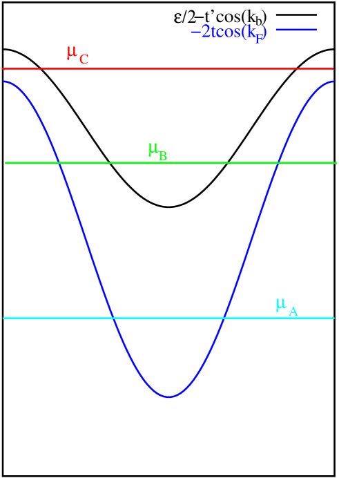
Figure 1: The different cases in the Bose-Fermi mixture with hardcore bosons when $\nu>0$. For $\mu=\mu_{A}$, the Fermion band is partially filled, and the hardcore boson band is empty. For $\mu=\mu_{C}$, the hardcore boson band is partially filled, and the fermion band is totally filled. In the case $\mu=\mu_{B}$, both band are partially filled. In the rest of the paper we will only consider the latter case.

Figure 2: The behavior of $k_{F}$ and $k_{B}$ for positive detuning $\nu>0$ as a function of the total density $\rho$. For low densities, only atoms are present ($k_{B}=0$). At higher densities such that $\pi\rho>2\sqrt{m_{F}\nu}$, a nonzero density of molecules appear. At the critical density, the slopes of $k_{F}$ and $k_{B}$ versus $\rho$ are discontinuous. On the figure we have taken $m_{F}\nu=1$.

Figure 3: The behavior of $k_{F}$ and $k_{B}$ for negative detuning $\nu<0$. For low densities, only the molecules are present ($k_{F}=0$). For $\pi\rho>4\sqrt{m_{F}|\nu|}$, molecules coexist with atoms. At the critical density, the slopes of $k_{F}$ and $k_{B}$ versus $\rho$ are discontinuous.

II.2.2 The case of bosons with finite repulsion

We have seen in the previous Section that in the case of hard core repulsion between the molecules, both in the lattice case and in the continuum case, that having $\nu<0$ did not prevent the formation of unpaired atoms provided the total density of atoms was large enough. This was related with the increase of the chemical potential of bosons as a result of repulsion when the density was increased. In this section, we want to analyze a slightly more realistic case where the repulsion between bosons is finite and check that coexistence remains possible. In the lattice case, the problem is untractable by analytic methods and one needs to rely on numerical approaches.Batrouni et al. (1990); Kühner et al. (2000) In the continuum case, however, it is well known that bosons with contact repulsions are exactly solvable by Bethe Ansatz techniques.Lieb and Liniger (1963) The density of molecules can therefore be obtained by solving a set of integral equations.Lieb and Liniger (1963); Takahashi (1997) They read:

$$\epsilon(k) = \frac{\hbar^{2}k^{2}}{2m_{B}}+\nu-\mu_{B}+\frac{c}{\pi}\int_{-q_{0}}^{q_{0}}\frac{dq}{c^{2}+(q-k)^{2}}\epsilon(q),$$ (15)

$$2\pi\rho(k) = 1+2c\int_{-q_{0}}^{q_{0}}\frac{\rho(q)dq}{c^{2}+(k-q)^{2}},$$ (16)

where:

$$c=\frac{m_{B}g_{BB}}{\hbar^{2}},$$ (17)

$$\rho_{B}=\int_{-q_{0}}^{q_{0}}\rho(q)dq,$$ (18)

$g_{BB}$ being the boson-boson interaction defined in Eq. (1). The parameter $q_{0}$ plays the role of a pseudo Fermi momentum. For $q>q_{0}$, we have $\rho(q)=0$. We also have $\epsilon(\pm q_{0})=0$.Lieb and Liniger (1963) It is convenient to introduce dimensionless variablesLieb and Liniger (1963):

$$\lambda=\frac{c}{q_{0}}\;;\;\gamma=\frac{c}{\rho_{B}},$$ (19)

and rewrite $k=q_{0}x$, $q=q_{0}y$, $\rho(q_{0}x)=g(x)$, $\epsilon(q_{0}x)=\frac{\hbar^{2}q_{0}^{2}}{2m}\bar{\epsilon}(x)$. The dimensionless integral equations read:

$$\bar{\epsilon}(x) = x^{2}+\frac{2m(\nu-\mu_{B})}{\hbar^{2}q_{0}^{2}}+\frac{\lambda}{\pi}\int_{-1}^{1}\frac{dy}{\lambda^{2}+(x-y)^{2}}\bar{\epsilon(y)},$$ (20)

$$2\pi g(x) = 1+2\lambda\int_{-1}^{1}\frac{g(y)dy}{\lambda^{2}+(x-y)^{2}}.$$ (21)

Using $\epsilon(\pm q_{0})=0$ one has the following integral equation for $\bar{\epsilon}(x)$:

$$\bar{\epsilon}(x)=x^{2}-1+\frac{\lambda}{\pi}\int_{-1}^{1}dy\bar{\epsilon}(y)\left[\frac{1}{\lambda^{2}+(x-y)^{2}}-\frac{1}{\lambda^{2}+(1-y)^{2}}\right]$$ (22)

Once this equation has been solved, the chemical potential of the bosons is obtained by:

$$\mu_{B}=\nu+\frac{\hbar^{2}q_{0}^{2}}{2m_{B}}\left[1+\frac{\lambda}{\pi}\int_{-1}^{1}\frac{1}{\lambda^{2}+(x-1)^{2}}\bar{\epsilon}(x)dx\right].$$ (23)

Knowing $\mu_{B}$ gives immediately $\mu_{F}=\mu_{B}/2$. From $\mu_{F}$ one finds $k_{F}=\sqrt{2m_{F}\mu_{F}}$ and $\rho_{F}=2k_{F}/\pi$. Finally, using the definition of the total density $\rho=2\rho_{B}+\rho_{F}$ one can map the molecule density and the free atom density as a function of the total density of atoms. The resulting equation of state can be written in terms of dimensionless parameters as:

$$\frac{\hbar^{2}\rho_{B}}{m_{B}g_{1D}}={\cal F}\left(\frac{\hbar^{2}\rho}{m_{B}g_{1D}},\frac{\hbar^{2}\nu}{m_{F}g_{1D}^{2}}\right)$$ (24)

The behavior of the boson density $\rho_{B}$ and fermion density $\rho_{F}$ as a function of total density $\rho$ can be understood in qualitative terms. Let us first discuss the case of negative detuning. For sufficiently low densities, only bosons are present. However, in that regime, the boson-boson repulsion is strong, and the boson chemical potential is increasing with the boson density. As a result, when the density exceeds a critical density $\rho_{c}$, the fermion chemical potential becomes positive, and the density of fermions becomes non-zero. The appearance of fermions is causing a cusp in the boson density plotted versus the total density. When the density of particles becomes higher, the boson-boson interaction becomes weaker, and the boson chemical potential barely increases with the density. As a result, the fermion density becomes almost independent of the total density. In the case of positive detuning, for low density, only fermions are present. Again, the increase of fermion density results in an increase of chemical potential and above a certain threshold in fermion density, bosons start to appear, creating a cusp in the dependence of the fermion density upon the total density. At large density, the detuning becomes irrelevant, and the fermion density barely increases with the total density.

To illustrate this behavior, we have solved numerically the integral equations (20), and calculated the resulting fermion and boson densities. A plot of the density of bosons as well as the density of fermions is shown on Fig. 4 for $\nu>0$ and on Fig. 5 for $\nu<0$. The slope discontinuities at the critical density remain visible. Obviously, this implies that the divergence of the compressibility is still present when the repulsion between the molecule is not infinite.

Figure 4: The density of molecules $\rho_{B}$ and unpaired atoms $\rho_{F}$ as a function of the total density $\rho$ in the case of a repulsion $c=100$ between the bosons and for positive detuning $\nu=0.1$. At large density, the fermion density is increasing more slowly than the boson density. Inset: the behavior of the boson and fermion densities near the origin. Note the cusp in the fermion density as the boson density becomes nonzero as in the $c=\infty$ case.

Figure 5: The density of molecules $\rho_{B}$ and unpaired atoms $\rho_{F}$ as a function of the total density $\rho$ in the case of a repulsion $c=100$ between the bosons and for negative detuning $\nu=-0.1$. At large density, the fermion density is increasing more slowly than the boson density. Inset: the behavior of the boson and fermion densities near the origin. Note the cusp in the boson density as the fermion density becomes nonzero as in the $c=\infty$ case.

We have thus seen that generally we should expect a coexistence of fermionic atoms and bosonic molecules as soon as repulsion between the molecules is sufficiently strong. Moreover, the repulsion between the molecules results in a finite velocity for sound excitations in the molecule Bose gas. As a result, we can expect that the gas of molecules will behave as a Luttinger liquid. Till now however, we have assumed that the term converting atoms into molecules was sufficiently small not to affect significantly the spectrum of the system. In the following, we will treat the effect of a small but not infinitesimal conversion term in Eqs. (2) and (1) using bosonization techniques. We will show that this term can lead to phase coherence between the atoms and the molecules, and we will discuss the properties of the phase in which such coherence is observed.

III Phase diagram and correlation functions

III.1 Derivation of the bosonized Hamiltonian

In this Section, we consider the case discussed in Sec. II where neither the density of molecules nor the density of atoms vanishes. As discussed in Sec. II, this requires a sufficiently large initial density of atoms. As there is both a non-zero density of atoms and of molecules, they both form Luttinger liquidsPetrov et al. (2004); Recati et al. (2003); Cazalilla (2003). These Luttinger liquids are coupled by the repulsion between atoms and molecules $V_{BF}$ and via the conversion term or Josephson coupling $\lambda$. To describe these coupled Luttinger liquids, we apply bosonizationGiamarchi (2004) to the Hamiltonians (2)– (1). For the sake of definiteness, we discuss the bosonization procedure in details only in the case of the continuum Hamiltonian (1). For the lattice Hamiltonian (2), the steps to follow are identical provided the system is not at a commensurate filling. At commensurate filling, umklapp terms must be added to the bosonized Hamiltonian and can result in Mott phasesGiamarchi (2004). This case is treated in Sec. IV.

To derive the bosonized Hamiltonian describing the low-energy spectrum of the Hamiltonian (1), we need first to consider the bosonized description of the system when all atom-molecule interactions are turned off. For $\lambda=0,V_{BF}=0$, both $N_{f}$ and $N_{b}$ are conserved and the bosonized Hamiltonian equivalent to (2) or (1) is given by:

$$H = H_{b}+H_{\rho}+H_{\sigma}$$

$$H_{b} = \int\frac{dx}{2\pi}\left[u_{b}K_{b}(\pi\Pi_{b})^{2}+\frac{u_{b}}{K_{b}}(\partial_{x}\phi_{b})^{2}\right]$$

$$H_{\rho} = \int\frac{dx}{2\pi}\left[u_{\rho}K_{\rho}(\pi\Pi_{\rho})^{2}+\frac{u_{\rho}}{K_{\rho}}(\partial_{x}\phi_{\rho})^{2}\right]$$

$$H_{\sigma} = \int\frac{dx}{2\pi}\left[u_{\sigma}K_{\sigma}(\pi\Pi_{\sigma})^{2}+\frac{u_{\sigma}}{K_{\sigma}}(\partial_{x}\phi_{\sigma})^{2}\right]-\frac{2g_{1\perp}}{(2\pi\alpha)^{2}}\int dx\cos\sqrt{8}\phi_{\sigma}$$ (25)

where $[\phi_{\nu}(x),\Pi_{\nu^{\prime}}(x^{\prime})]=i\delta(x-x^{\prime})\delta_{\nu,\nu^{\prime}}$, ($\nu,\nu^{\prime}=b,\sigma,\rho$). In the context of cold atoms, the Hamiltonian (III.1) have been discussed in Cazalilla (2003); Recati et al. (2003); Petrov et al. (2004). The parameters $K_{\rho}$, the Luttinger exponent, and $u_{\rho},u_{\sigma}$, the charge and spin velocities, are known functions of the interactions Gaudin (1967); Schulz (1990); Frahm and Korepin (1990), with $K_{\rho}=1$ in the non-interacting case, $g_{1\perp}$ is a marginally irrelevant interaction, and at the fixed point of the RG flow $K_{\sigma}^{*}=1$. For the bosonic system, the parameters $u_{b},K_{b}$ can be obtained from numerical calculationsKühner et al. (2000) in the lattice case or from the solution of the Lieb-Liniger modelLieb and Liniger (1963) in the continuum case. In the case of non-interacting bosons $K_{b}\to\infty$ and in the case of hard core bosons $K_{b}=1$.Girardeau (1960); Schultz (1963); Haldane (1981) An important property of the parameters $K_{b}$ and $K_{\rho}$ is that they decrease as (respectively) the boson-boson and fermion-fermion interaction become more repulsive. The bosonized Hamiltonian (III.1) is also valid in the lattice case (2) provided that both $N_{f}$ and $N_{b}$ do not correspond to any commensurate filling.

The fermion operators can be expressed as functions of the bosonic fields appearing in (III.1) as Giamarchi (2004):

$$\psi_{\sigma}(x)=\sum_{r=\pm}e^{irk_{F}n\alpha}\psi_{r,\sigma}(x=n\alpha)$$ (26)

$$\psi_{r,\sigma}(x)=\frac{e^{\frac{i}{\sqrt{2}}[\theta_{\rho}-r\phi_{\rho}+\sigma(\theta_{\sigma}-r\phi_{\sigma})](x)}}{\sqrt{2\pi\alpha}},$$ (27)

where the index $r=\pm$ indicates the right/left movers, $\alpha$ is a cutoff equal to the lattice spacing in the case of the model Eq. (2). Similarly, the boson operators are expressed asGiamarchi (2004):

$$\frac{b_{n}}{\sqrt{\alpha}}=\Psi_{b}(x=n\alpha)$$ (28)

$$\Psi_{b}(x)=\frac{e^{i\theta_{b}}}{\sqrt{2\pi\alpha}}\left[1+A\cos(2\phi_{b}-2k_{B}x)\right].$$ (29)

In Eqs. (26)-(28), we have introduced the dual fieldsGiamarchi (2004) $\theta_{\nu}(x)=\pi\int^{x}\Pi_{\nu}(x^{\prime})dx^{\prime}$ ($\nu=\rho,\sigma,b$), $k_{F}=\pi N_{f}/2L$, and $k_{B}=\pi N_{b}/L$ where $L$ is the length of the system. The fermion density is given byGiamarchi (2004):

$$\sum_{\sigma}\frac{n_{f,n,\sigma}}{\alpha}=\rho_{f}(x=n\alpha)=-\frac{\sqrt{2}}{\pi}\partial_{x}\phi_{\rho}+\frac{\cos(2k_{F}x-\sqrt{2}\phi_{\rho})}{\pi\alpha}\cos\sqrt{2}\phi_{\sigma},$$ (30)

and the boson density byGiamarchi (2004):

$$\frac{n_{b,n}}{a}=\rho_{b}(x)=-\frac{1}{\pi}\partial_{x}\phi_{b}+\frac{\cos(2k_{B}x-2\phi_{b})}{\pi\alpha}.$$ (31)

The detuning term in (1) is thus expressed as:

$$H_{detuning}=-\frac{\nu}{\pi}\int dx\partial_{x}\phi_{b}$$ (32)

We now turn on a small $\lambda$ and a small $V_{BF}$. The effect of a small $V_{BF}$ on a boson-fermion mixture has been investigated previouslyCazalilla and Ho (2003); Mathey et al. (2004). The forward scattering contribution is:

$$\frac{V_{BF}\sqrt{2}}{\pi^{2}}\int\partial_{x}\phi_{b}\partial_{x}\phi_{\rho},$$ (33)

and as discussed in Cazalilla and Ho (2003), it can give rise to a phase separation between bosons and fermions if it is too repulsive. Otherwise, it only leads to a renormalization of the Luttinger exponents. The atom molecule repulsion term also gives a backscattering contribution:

$$\frac{2V_{BF}}{(2\pi\alpha)^{2}}\int dx\cos(2\phi_{b}-\sqrt{2}\phi_{\rho}-2(k_{F}-k_{B})x)\cos\sqrt{2}\phi_{\sigma},$$ (34)

however in the general case, $k_{F}\neq k_{B}$ this contribution is vanishing. In the special case of $k_{B}=k_{F}$, the backscattering can result in the formation of a charge density wave. This effect will be discussed in Sec. III.2.3. The contribution of the $\lambda$ term is more interesting.Sheehy and Radzihovsky (2005); Citro and Orignac (2005) Using Eqs. (26)-(28), we find that the most relevant contribution reads:

$$H_{bf}=\frac{2\lambda}{\sqrt{2\pi^{3}\alpha^{3}}}\int dx\cos(\theta_{b}-\sqrt{2}\theta_{\rho})\cos\sqrt{2}\phi_{\sigma}$$ (35)

In the next section, we will see that this term gives rise to a phase with atom-molecule coherence when the repulsion is not too strong.

III.2 Phase diagram

III.2.1 phase with atom-molecule coherence

The effect of the term (35) on the phase diagram can be studied by renormalization group techniquesGiamarchi (2004). A detailed study of the renormalization group equations has been published in Sheehy and Radzihovsky (2005). Here, we present a simplified analysis, which is sufficient to predict the phases that can be obtained in our system. The scaling dimension of the boson-fermion coupling term (35) is: $\frac{1}{4K_{b}}+\frac{1}{2K_{\rho}}+\frac{1}{2}K_{\sigma}$. For small $\lambda$ it is reasonable to replace $K_{\sigma}$ with its fixed point value $K_{\sigma}^{*}=1$. Therefore, the RG equation for the dimensionless coupling $\tilde{\lambda}=\frac{\lambda\alpha^{1/2}}{u}$ (where $u$ is one of the velocities $u_{\rho},u_{\sigma},u_{b}$) reads:

$$\frac{d\tilde{\lambda}}{d\ell}=\left(\frac{3}{2}-\frac{1}{2K_{\rho}}-\frac{1}{4K_{b}}\right)\tilde{\lambda},$$ (36)

where $\ell$ is related to the renormalized cutoff $\alpha(\ell)=\alpha e^{\ell}$. We thus see that for $\frac{1}{2K_{\rho}}+\frac{1}{4K_{b}}<3/2$, this interaction is relevant. Since for hardcore bosonsGirardeau (1960); Schultz (1963) $K_{b}=1$ and for non-interacting bosons $K_{b}=\infty$, while for free fermions $K_{\rho}=1$ and in the lattice case for $U=\infty$ one has $K_{\rho}=1/2$Kawakami and Yang (1990), we see that the inequality is satisfied unless there are very strongly repulsive interactions both in the boson system and in the fermion system. When this inequality is not satisfied, for instance in the case of fermions with nearest-neighbor repulsionMila and Zotos (1993); Sano and Ōno (1994), in which one can have $1/4<K_{\rho}<1/2$ and hardcore bosons with nearest neighbor repulsionShankar (1990); Haldane (1980), in which one can have $K_{b}=1/2$, the atoms and the molecules decouple. This case is analogous to that of the mixture of bosons and fermionsMathey et al. (2004); Cazalilla and Ho (2003)and charge density waves can be formed if $k_{B}$ and $k_{F}$ are commensurate. The phase transition between this decoupled phase and the coupled phase belongs to the Berezinskii-Kosterlitz-Thouless (BKT) universality class.Kosterlitz and Thouless (1973) As pointed out in Sheehy and Radzihovsky (2005), in the decoupled phase, the effective interaction between the fermions can be attractive. In that case, a spin gap is formed Luther and Emery (1974); Giamarchi (2004) and the fermions are in a Luther-Emery liquid state with gapless density excitations. Let us consider the coupled phase in more details. The relevance of the interaction (35) leads to the locking of $\phi_{\sigma}$, i.e. it results in the formation of a spin gap. To understand the effect of the term $\cos(\theta_{b}-\sqrt{2}\theta_{\rho})$, it is better to perform a rotation:

$$\left(\begin{array}[]{c}\theta_{-}\\ \theta_{+}\end{array}\right)=\left(\begin{array}[]{cc}\frac{1}{\sqrt{3}}&-\frac{\sqrt{2}}{\sqrt{3}}\\ \frac{\sqrt{2}}{\sqrt{3}}&\frac{1}{\sqrt{3}}\end{array}\right)\left(\begin{array}[]{c}\theta_{b}\\ \theta_{\rho}\end{array}\right),$$ (37)

and the same transformation for the $\phi_{\nu}$. This transformation preserves the canonical commutation relations between $\phi_{\pm}$ and $\Pi_{\pm}$. Under this transformation, $H_{b}+H_{\rho}$ becomes:

$$H_{b}+H_{\rho} = \int\frac{dx}{2\pi}\sum_{\nu=\pm}\left[u_{\nu}K_{\nu}(\pi\Pi_{\nu})^{2}+\frac{u_{\nu}}{K_{\nu}}(\partial_{x}\phi_{\nu})^{2}\right]$$ (38)

$$+\int\frac{dx}{2\pi}[g_{1}(\pi\Pi_{+})(\pi\Pi_{-})+g_{2}\partial_{x}\phi_{+}\partial_{x}\phi_{-}],$$

where:

$$u_{+}K_{+} = \frac{2}{3}u_{b}K_{b}+\frac{1}{3}u_{\rho}K_{\rho},$$

$$u_{-}K_{-} = \frac{1}{3}u_{b}K_{b}+\frac{2}{3}u_{\rho}K_{\rho},$$

$$g_{1} = \frac{\sqrt{8}}{3}(u_{b}K_{b}-u_{\rho}K_{\rho}),$$

$$\frac{u_{+}}{K_{+}} = \frac{2u_{b}}{3K_{b}}+\frac{u_{\rho}}{3K_{\rho}}+\frac{4V}{3\pi},$$ (39)

$$\frac{u_{-}}{K_{-}} = \frac{u_{b}}{3K_{b}}+\frac{2u_{\rho}}{3K_{\rho}}-\frac{4V}{3\pi},$$ (40)

$$g_{2} = \frac{\sqrt{8}}{3}(\frac{u_{b}}{K_{b}}-{u_{\rho}}{K_{\rho}}-\frac{V}{\pi}),$$ (41)

while, $H_{bf}$ defined in (35) becomes:

$$H_{bf}=\frac{\lambda}{\sqrt{2\pi^{3}}\alpha}\int dx\cos\sqrt{3}\theta_{-}\cos\sqrt{2}\phi_{\sigma}.$$ (42)

After the rotation, we see that when $\lambda$ is relevant, the field $\theta_{-}$ is also locked, but $\phi_{+}$ remains gapless. Since the field $\theta_{-}$ is the difference of the superfluid phase of the atoms and the one of the molecules, this means that when $\lambda$ becomes relevant, unpaired atoms and molecules share the same superfluid phase i.e. they become coherent. The gap induced by the term $\lambda$ can be estimated from the renormalization group equation (36). Under the renormalization group, the dimensionless parameter $\tilde{\lambda}(\ell)$ grows until it becomes of order one at a scale $\ell=\ell^{*}$ where the perturbative approach breaks down. Beyond the scale $\ell^{*}$, the fields $\theta_{-}$ and $\phi_{\sigma}$ behave as classical fields. Therefore, the associated energy scale $u/(\alpha e^{\ell^{*}})$ is the scale of the gap. From this argument, we obtain that the gap behaves as:

$$\Delta\sim\frac{u}{\alpha}\left(\frac{\lambda\alpha^{1/2}}{u}\right)^{\frac{1}{\frac{3}{2}-\frac{1}{2K_{\rho}}-\frac{1}{4K_{b}}}}.$$ (43)

The gapful excitations have a dispersion $\epsilon(k)=\sqrt{(uk)^{2}+\Delta^{2}}$ and are kinks and antikinks of the fields $\theta_{-}$ and $\phi_{\sigma}$.Rajaraman (1982) More precisely, since a kink must interpolate between degenerate classical ground states of the potential (42), we find that when a kink is present $\theta_{-}(+\infty)-\theta_{-}(-\infty)=\pm\pi/\sqrt{3}$ and $\phi_{\sigma}(+\infty)-\phi_{\sigma}(-\infty)=\pi/\sqrt{2}$. This indicates that a kink is carrying a spin $1/2$, and is making the phase $\theta_{b}$ of the bosons jump by $\pi/3$ and the phase of the superfluid order parameter $\sqrt{2}\theta_{\rho}$ of the fermions jump by $-2\pi/3$. Since the current of bosons is $j_{b}=u_{b}K_{b}\pi\Pi_{b}=u_{b}K_{b}\partial_{x}\theta_{b}$ and the current of fermions is $j_{F}=\sqrt{2}u_{\rho}K_{\rho}\pi\Pi_{\rho}=\sqrt{2}u_{\rho}K_{\rho}\partial_{x}\theta_{\rho}$, this indicates that counterpropagating supercurrents of atoms and molecules exist in the vicinity of the kinks. Therefore, we can view the kinks and antikinks are composite objects formed of vortices bound with a spin 1/2. We note that the kinks and antikinks may not exhaust all the possible gapful excitations of the system. In particular, bound states of kinks and antikinks, known as breathers may also be presentRajaraman (1982). However, these gapful excitations present a larger gap than the single kinks. Let us now turn to the gapless field $\phi_{+}$. This field has a simple physical interpretation. Considering the integral

$$-\frac{1}{\pi}\int_{-\infty}^{\infty}dx\partial_{x}\phi_{+} = -\frac{1}{\pi\sqrt{3}}\int_{-\infty}^{\infty}(\sqrt{2}\phi_{b}+\phi_{\rho})=\frac{\mathcal{N}}{\sqrt{6}},$$ (44)

showing that $\phi_{+}(\infty)-\phi_{+}(-\infty)$ measures the total number of particles in the system $\mathcal{N}$. Thus $(\Pi_{+},\phi_{+})$ describe the total density excitations of the system.

The resulting low-energy Hamiltonian describing the gapless total density modes reads:

$$H_{+}=\int\frac{dx}{2\pi}\left[u^{*}_{+}K^{*}_{+}(\pi\Pi_{+})^{2}+\frac{u^{*}_{+}}{K^{*}_{+}}(\partial_{x}\phi_{+})^{2}\right],$$ (45)

where $u^{*}_{+},K^{*}_{+}$ denote renormalized values of $u_{+},K_{+}$. This renormalization is caused by the residual interactions between gapless modes and the gapped modes measured by $g_{1},g_{2}$ in Eq. (38). Since $\phi_{+}$ measures the total density, the Hamiltonian (45) describes the propagation of sound modes in the 1D fluid with dispersion $\omega(k)=u|k|$. We note than in Ref.Zhou (2005); Zhou and Wu (2005), dispersion relation similar to ours were derived for the sound modes and the superfluid phase difference modes using different methods.

III.2.2 effect of the detuning and applied magnetic field

Having understood the nature of the ground state and the low excited states when $\lambda$ is relevant we turn to the effect of the detuning term. Eqs. (32) and (37) show that the detuning term can be expressed as a function of $\phi_{+},\phi_{-}$ as:

$$H_{detun.}=-\frac{\nu}{\pi}\int\partial_{x}\left(\sqrt{\frac{2}{3}}\phi_{+}+\frac{\phi_{-}}{\sqrt{3}}\right).$$ (46)

This shows that the detuning does not affect the boson-fermion coupling (35) since it can be eliminated from the Hamiltonian by a canonical transformation $\phi_{\pm}\to\phi_{\pm}+\lambda_{\pm}x$, where $\lambda_{+}=\nu\sqrt{\frac{2}{3}}$ and $\lambda_{-}=\nu\frac{1}{\sqrt{3}}$. For a fixed total density, changing the detuning only modifies the wavevectors $k_{B}$ and $k_{F}$. As discussed extensively in Sec. II.2, for a detuning sufficiently large in absolute value, only molecules or only atoms are present, and near the critical value of the detuning, the compressibility of the system is divergent. We therefore conclude that in one-dimension, the crossover from the Bose condensation to the superfluid state, as the detuning is varied, is the results of the band-filling transitions at which either the density of the atoms or the molecules goes to zero. At such band filling transitions,$v_{\rho,\sigma}\to 0$ (respectively $v_{b}\to 0$) and bosonization breaks down Nomura (1996); Cabra and Drut (2003); Yang (2004). The two band filling transitions are represented on Fig. 6. The cases at the extreme left and the extreme right of the phase diagram have been analyzed in Fuchs et al. (2005), where it was shown that in the case of a broad Fano-Feshbach resonance, the zone of coexistence was very narrow. In the narrow Fano-Feshbach resonance case we are investigating, the zone of coexistence can be quite important.

Figure 6: The band filling transitions as a function of the detuning

Application of a magnetic field can also induce some phase transitions. The interaction with the magnetic field reads:

$$H_{magn}=-\frac{h}{\pi\sqrt{2}}\int dx\partial_{x}\phi_{\sigma},$$ (47)

The effect of the magnetic field is to lower the gap for the creation of kink excitations (remember that they carry a spin $1/2$). As a result, when it becomes larger than the gap, the magnetic field induces a commensurate incommensurate transitionJaparidze and Nersesyan (1978); Pokrovsky and Talapov (1979); Schulz (1980); Horowitz et al. (1983) that destroys the coherence between atoms and molecules and gives back decoupled Luttinger liquidsChitra and Giamarchi (1997). In that regime, the behavior of the system is described by the models of Ref. Cazalilla and Ho, 2003; Mathey et al., 2004. Commensurate-incommensurate transitions have been already discussed in the context of cold atoms in Büchler et al. (2003). In the problem we are considering, however , since two fields are becoming gapless at the same time, $\theta_{-}$ and $\phi_{\sigma}$ , there are some differencesOrignac et al. (2000); Yu and Haas (2001) with the standard caseBüchler et al. (2003), in particular the exponents at the transition are non-universal.

To conclude this section, we notice that we have found three types of phase transitions in the system we are considering. We can have Kosterlitz-Thouless phase transitions as a function of interactions, where we go from a phase with locked superfluid phases between the bosons and the fermions at weak repulsion to a phase with decoupled bosons and fermions at strong repulsion. We can have band-filling transitions as a function of the detuning between the phase in which atoms and molecule coexist and phases where only atoms or only molecules are present. Finally, we can have commensurate-incommensurate transitions as a function of the strength of the magnetic field. In the following section, we discuss the correlation functions of superfluid and charge density wave order parameters in the phase in which molecules and atoms coexist with their relative superfluid phase $\theta_{-}$ locked.

III.2.3 Quantum Ising phase transition for $k_{F}=k_{B}$

In the case of $k_{F}=k_{B}$, the backscattering term (34) is non-vanishing. This term induces a mutual locking of the densities of the bosons and the fermionsCazalilla and Ho (2003) and favors charge density wave fluctuations. This term is competing with the Josephson term (35) which tends to reduce density wave fluctuations. For $k_{F}=k_{B}$ the relevant part of the Hamiltonian given by the combination of the terms (34) and (35) reads:

$$H_{\text{Josephon}+\text{CDW Lock.}}=\int dx\left[\frac{2\lambda}{\sqrt{2\pi^{3}\alpha^{3}}}\cos(\theta_{b}-\sqrt{2}\theta_{\rho})+\frac{2V_{BF}}{(2\pi\alpha)^{2}}\cos(2\phi_{b}-\sqrt{2}\phi_{\rho})\right]\cos\sqrt{2}\phi_{\sigma}$$ (48)

Using a transformation $\phi_{b}=\tilde{\phi}_{b}/\sqrt{2}$, $\theta_{b}=\tilde{\theta}_{b}\sqrt{2}$, and introducing the linear combinations

$$\phi_{1}=\frac{\tilde{\phi}_{b}+\phi_{\rho}}{\sqrt{2}}$$ (49)

$$\phi_{2}=\frac{\tilde{\phi}_{b}-\phi_{\rho}}{\sqrt{2}}$$ (50)

and similar combinations for the dual fields, we can rewrite the interaction term (48) as:

$$H_{\text{Josephon}+\text{CDW Lock.}}=\int dx\left[\frac{2\lambda}{\sqrt{2\pi^{3}\alpha^{3}}}\cos 2\theta_{2}+\frac{2V_{BF}}{(2\pi\alpha)^{2}}\cos 2\phi_{2}\right]\cos\sqrt{2}\phi_{\sigma}$$ (51)

From this Hamiltonian, it is immediate to see that a quantum Ising phase transition occurs between the density wave phase $\phi_{2}$ and the superfluid phase $\theta_{2}$ at a critical point $\lambda_{c}=\frac{V_{BF}}{\sqrt{8\pi\alpha}}$.Finkelstein and Larkin (1993); Schulz (1996); Fabrizio et al. (2000) Indeed, the field $\phi_{\sigma}$ being locked, we can replace $\cos\sqrt{2}\phi_{\sigma}$ by its expectation value in Eq. (51), and rewrite (51) as a free massive Majorana fermions Hamiltonian.Finkelstein and Larkin (1993); Schulz (1996); Fabrizio et al. (2000) At the point $\lambda_{c}$, the mass of one of these Majorana fermions vanishes giving a quantum critical point in the Ising universality classSachdev (2000). On one side of the transition, when $\lambda>\lambda_{c}$, the system is in the superfluid state discussed in Sec. III.2, on the other side $\lambda<\lambda_{c}$, the charge density wave state discussed in Cazalilla and Ho (2003) is recovered.

III.3 Correlation functions

In order to better characterize the phase in which $\lambda$ is relevant, we need to study the correlation function of the superfluid and the charge density wave operators. Let us begin by characterizing the superfluid order parameters. First, let us consider the order parameter for BEC of the molecules. As a result of the locking of the fields $\theta_{-}$ and $\phi_{\sigma}$, the boson operator Eq. (28) becomes at low energy:

$$\Psi_{B}(x)\sim\frac{e^{i\sqrt{\frac{2}{3}}\theta_{+}}}{\sqrt{2\pi\alpha}}\left\langle e^{-i\frac{\theta_{-}}{\sqrt{3}}}\right\rangle.$$ (52)

An order of magnitude of $\langle e^{-i\frac{\theta_{-}}{\sqrt{3}}}\rangle$ can be obtained from a scaling argument similar to the one giving the gap. Since the scaling dimension of the field $e^{-i\frac{\theta_{-}}{\sqrt{3}}}$ is $1/12K_{-}$, and since the only lengthscale in the problem is $e^{\ell^{*}}$, we must have $\langle e^{-i\frac{\theta_{-}}{\sqrt{3}}}\rangle\sim e^{-\ell^{*}/12K_{-}}\sim(\lambda\alpha^{1/2}/u)^{1/12K_{-}}$. Similarly, the order parameter for s-wave superconductivity of the atoms $O_{SS}=\sum_{\sigma}\psi_{r,\sigma}\psi_{-r,-\sigma}$ becomes:

$$O_{SS}=\frac{e^{i\sqrt{2}\theta_{\rho}}}{\pi\alpha}\cos\sqrt{2}\phi_{\sigma}\sim\frac{e^{i\sqrt{\frac{2}{3}}\theta_{+}}}{\pi\alpha}\left\langle e^{\frac{2i}{\sqrt{3}}\theta_{-}}\cos\sqrt{2}\phi_{\sigma}\right\rangle,$$ (53)

thus indicating that the order parameters of the BEC and the BCS superfluidity have become identical in the low energy limitOhashi and Griffin (2003a, b). This is the signature of the coherence between the atom and the molecular superfluids. The boson correlator behaves as:

$$\langle\Psi_{B}(x,\tau)\Psi_{B}(0,0)=\left(\frac{\alpha^{2}}{x^{2}+(u\tau)^{2}}\right)^{\frac{1}{6K_{+}}}$$ (54)

As a result, the molecule momentum distribution becomes $n_{B}(k)\sim|k|^{1/(3K_{+})-1}$. One can see that the tendency towards superfluidity is strongly enhanced since the divergence of $n_{B}(k)$ for $k\to 0$ is increased by the coherence between the molecules and the atoms. This boson momentum distribution can, in principle be measured in a condensate expansion experimentGerbier et al. (2005); Altman et al. (2004).

Having seen that superfluidity is enhanced in the system, with BEC and BCS order parameters becoming identical, let us turn to the density wave order parameters. These order parameters are simply the staggered components of the atom and molecule density in Eqs. (30)–(31). In terms of $\phi_{\pm}$, the staggered component of the molecule density is reexpressed as:

$$\rho_{2k_{B},b}(x)\sim\cos\left[2\left(\frac{\phi_{-}}{\sqrt{3}}+\frac{\sqrt{2}}{\sqrt{3}}\phi_{+}\right)-2k_{b}x\right],$$ (55)

and the staggered component of the fermion density as:

$$\rho_{2k_{F},f}(x)\sim\cos\left[\sqrt{2}\left(-\frac{\sqrt{2}}{\sqrt{3}}\phi_{-}+\frac{1}{\sqrt{3}}\phi_{+}\right)-2k_{F}x\right],$$ (56)

where we have taken into account the long range ordering of $\phi_{\sigma}$. We see that the correlations of both $\rho_{2k_{B},b}(x)$ and $\rho_{2k_{F},f}(x)$ decay exponentially due to the presence of the disorder field $\phi_{-}$ dual to $\theta_{-}$. In more physical terms, the exponential decay of the density-wave correlations in the system results from the constant conversion of molecules into atoms and the reciprocal process which prevents the buildup of a well defined atomic Fermi-surface or molecule pseudo-Fermi surface. The exponential decay of the density wave correlations in this system must be be contrasted with the power-law decay of these correlations in a system with only bosons or in a system of fermions with attractive interactions.Giamarchi (2004) In fact, if we consider that our new particles are created by the operator $\psi_{b}\sim\psi_{\uparrow}\psi_{\downarrow}$, we can derive an expression of the density operators of these new particles by considering the product $\psi_{b}\psi_{\uparrow}\psi_{\downarrow}$. Using the Haldane expansion of the boson creation and annihilation operatorsHaldane (1981); Lukyanov and Terras (2003), we can write this product as:

$$\psi^{\dagger}_{b}\psi_{\uparrow}\psi_{\downarrow} \sim e^{-i\theta_{b}}\left[\sum_{m=0}^{\infty}\cos(2m\phi-2mk_{B}x)\right]\times e^{i\sqrt{2}\theta_{\rho}}\left[\cos\sqrt{2}\phi_{\sigma}+\cos(\sqrt{2}\phi_{\rho}-2k_{F}x)\right]$$ (57)

$$\sim \langle e^{-i(\theta_{b}-\sqrt{2}\theta_{\rho})}\cos\sqrt{2}\phi_{\sigma}\rangle\cos(\sqrt{6}\phi_{+}-2(k_{F}+k_{B})x),$$

where $(k_{F}+k_{B})=\pi(2N_{b}+N_{f})/2L=\pi\rho_{pairs}$ can be interpreted as the pseudo Fermi wavevector of composite bosons. A scaling argument shows that the prefactor in the expression varies as a power of $\lambda$. As a result, when there is coherence between atoms and molecule, power-law correlations appear in the density-density correlator near the wavevector $2k_{F}+2k_{B}$ and the intensity of these correlations is proportional to the $|\langle e^{-i(\theta_{b}-\sqrt{2}\theta_{\rho})}\cos\sqrt{2}\phi_{\sigma}\rangle|^{2}$. The resulting behavior of the Fourier transform of the density-density correlator is represented on Fig. 7.

Figure 7: Fourier transform of the static density density correlations. In the decoupled phase (dashed line), two peaks are obtained at twice the Fermi wavevector of the unpaired atoms and at twice the pseudo-Fermi wavevector of the molecules. In the coupled phase (solid line), the peaks are replaced by maxima at $Q=2k_{F}$ and $Q=2k_{B}$. A new peak at $Q=2(k_{F}+k_{B})$ is obtained as a result of Boson-Fermion coherence.

Another interesting consequence of the existence of atom/molecule coherence is the possibility of having non-vanishing cross-correlations of the atom and the molecule density. In the three-dimensional case such cross correlations have been studied in Ohashi and Griffin (2005). If we first consider cross-correlations $\langle T_{\tau}\rho_{2k_{B},b}(x,\tau)\rho_{2k_{F},f}(0,0)\rangle$ we notice that due to the presence of different exponentials of $\phi_{+}$ in Eqs. (55)– (56), this correlator vanishes exactly. Therefore, no cross correlation exists between the staggered densities. However, if we consider the cross correlations of the uniform densities, we note that since they can all be expressed as functions of $\partial_{x}\phi_{+},\partial_{x}\phi_{-}$, such cross correlations will be non-vanishing. More precisely, since:

$$\rho_{F} = -\frac{\sqrt{2}}{\pi\sqrt{3}}\partial_{x}\phi_{+}+\frac{2}{\pi\sqrt{3}}\partial_{x}\phi_{-}$$ (58)

$$\rho_{B} = -\frac{\sqrt{2}}{\pi\sqrt{3}}\partial_{x}\phi_{+}-\frac{1}{\pi\sqrt{3}}\partial_{x}\phi_{-},$$ (59)

at low energy we have: $\rho_{F}\sim\rho_{B}\sim-\frac{\sqrt{2}}{\pi\sqrt{3}}\partial_{x}\phi_{+}$.

III.4 The Luther Emery point

In this Section, we will obtain detailed expressions for these correlation functions at a special exactly solvable point of the parameter space. At this point, the kinks of the fields $\phi_{\sigma}$ and $\theta_{-}$ become free massive fermions. This property, and the equivalence of free massive fermions in 1D with the 2D non-critical Ising modelLuther and Peschel (1975); Zuber and Itzykson (1977); Schroer and Truong (1978); Kadanoff (1979); Ogilvie (1981); Boyanovsky (1989); Itzykson and Drouffe (1989) allows one to find exactly the correlation functions.

III.4.1 mapping on free fermions

As we have seen, after the rotation (37), if we neglect the interaction terms of the form $\Pi_{+}\Pi_{-}$ or $\partial_{x}\phi_{+}\partial_{x}\phi_{-}$, the Hamiltonian of the massive modes $\phi_{-},\phi_{\sigma}$ can be rewritten as:

$$H = \int\frac{dx}{2\pi}\left[u_{\sigma}^{*}K_{\sigma}^{*}(\pi\Pi_{\sigma})^{2}+\frac{u_{\sigma}^{*}}{K_{\sigma}^{*}}(\partial_{x}\phi_{\sigma})^{2}\right]$$ (60)

$$+\int\frac{dx}{2\pi}\left[u_{-}K_{-}(\pi\Pi_{-})^{2}+\frac{u_{-}}{K_{-}}(\partial_{x}\phi_{-})^{2}\right]$$

$$+\frac{\lambda}{\sqrt{2\pi^{3}\alpha^{3}}}\int dx\cos\sqrt{3}\theta_{-}\cos\sqrt{2}\phi_{\sigma},$$

where $K_{\sigma}^{*}=1$. When the Luttinger exponent is $K_{-}=3/2$, it is convenient to introduce the fields:

$$\overline{\phi}=\sqrt{\frac{3}{2}}\theta_{-}$$ (61)

$$\overline{\theta}=\sqrt{\frac{2}{3}}\phi_{-},$$ (62)

and rewrite the Hamiltonian (60) as:

$$H = \int\frac{dx}{2\pi}\left[u_{\sigma}^{*}(\pi\Pi_{\sigma})^{2}+{u_{\sigma}^{*}}(\partial_{x}\phi_{\sigma})^{2}\right]$$ (63)

$$+\int\frac{dx}{2\pi}\left[u_{-}(\pi\overline{\Pi})^{2}+{u_{-}}(\partial_{x}\overline{\phi})^{2}\right]$$

$$+\frac{\lambda}{\sqrt{2\pi^{3}}\alpha}\int dx\cos\sqrt{2}\overline{\phi}\cos\sqrt{2}\phi_{\sigma}.$$

If we neglect the velocity difference, i.e. assume that $u_{\sigma}^{*}=u_{-}=u$, and introduce the pseudofermion fields:

$$\Psi_{r,\sigma}=\frac{e^{i[(\overline{\theta}-r\overline{\phi})+\sigma(\theta_{\sigma}-r\phi_{\sigma})]}}{\sqrt{2\pi\alpha}},$$ (64)

we see immediately that the Hamiltonian (63) is the bosonized form of the following free fermion Hamiltonian:

$$H=\sum_{\sigma}\int dx\left[-iu\sum_{r=\pm}r\Psi_{r,\sigma}^{\dagger}\partial_{x}\Psi_{r,\sigma}+\frac{\lambda}{\sqrt{2\pi\alpha}}\Psi_{r,\sigma}^{\dagger}\Psi_{r,\sigma}\right].$$ (65)

As a result, for the special value of $K_{-}=3/2$, the excitations can be described as massive free fermions with dispersion $\epsilon(k)=\sqrt{(uk)^{2}+m^{2}}$, where $m=\frac{|\lambda|}{\sqrt{2\pi\alpha}}$. This is known as Luther-Emery solution.Luther and Emery (1974); Coleman (1975) One can see that the fermions carry a spin $1/2$ and a jump of the phase $\theta_{-}$ equal to $\frac{\pi}{\sqrt{3}}$. Therefore they can be identified to the kinks obtained in the semiclassical treatment of Sec. III.2. Also, making all velocities equal and $V_{BF}=0$ in (III.2.1), we find the relation $3/K_{-}=1/K_{b}+2/K_{\rho}$ and thus the gap given by the RG varies as $\Delta\sim\frac{u}{\alpha}\left(\frac{\lambda\alpha^{1/2}}{u}\right)^{\frac{1}{\frac{3}{2}-\frac{3}{4K_{-}}}}$. For $K_{-}=3/2$ this expression reduces to the one given by the fermion mapping.

III.4.2 Correlation functions

To calculate the correlation functions it is convenient to introduce the fields:

$$\Phi_{\sigma} = \frac{1}{\sqrt{2}}(\overline{\phi}+\sigma\phi_{\sigma})$$ (66)

$$\Theta_{\sigma} = \frac{1}{\sqrt{2}}(\overline{\theta}+\sigma\theta_{\sigma})$$ (67)

And reexpress operators by:

$$e^{i\frac{2}{\sqrt{3}}\phi_{-}} = e^{i(\Theta_{\uparrow}+\Theta_{\downarrow})}$$

$$e^{i\sqrt{2}\phi_{\sigma}}e^{-i\frac{2}{\sqrt{3}}\phi_{-}} = e^{i(\Phi_{\uparrow}-\Phi_{\downarrow})}e^{-i(\Theta_{\uparrow}+\Theta_{\downarrow})}\sim\Psi^{\dagger}_{+,\uparrow}\Psi^{\dagger}_{-,\downarrow}$$

$$e^{-i\sqrt{2}\phi_{\sigma}}e^{-i\frac{2}{\sqrt{3}}\phi_{-}} = e^{-i(\Phi_{\uparrow}-\Phi_{\downarrow})}e^{-i(\Theta_{\uparrow}+\Theta_{\downarrow})}\sim\Psi^{\dagger}_{-,\uparrow}\Psi^{\dagger}_{+,\downarrow}$$ (68)

This leads us to the following expression of the fermion density $\rho_{2k_{F},f}(x)$:

$$\rho_{2k_{F},f}(x)=e^{i\left[\sqrt{\frac{2}{3}}\phi_{+}-2k_{F}x\right]}(\Psi^{\dagger}_{-,\uparrow}\Psi^{\dagger}_{+,\downarrow}+\Psi^{\dagger}_{+,\uparrow}\Psi^{\dagger}_{-,\downarrow})+\text{H. c.},$$ (69)

which enables us to find exactly its correlations. We introduce $u=u_{\sigma}^{*}$ to simplify the notations. The Green’s functions of the fermions read:

$$G_{++}(x,\tau) = -\frac{m}{2\pi u}\frac{\tau+i\frac{x}{u}}{\sqrt{\tau^{2}+\frac{x^{2}}{u^{2}}}}K_{1}\left(m\sqrt{\tau^{2}+\left(\frac{x}{u}\right)^{2}}\right)$$ (70)

$$G_{--}(x,\tau) = -\frac{m}{2\pi u}\frac{\tau-i\frac{x}{u}}{\sqrt{\tau^{2}+\frac{x^{2}}{u^{2}}}}K_{1}\left(m\sqrt{\tau^{2}+\left(\frac{x}{u}\right)^{2}}\right)$$ (71)

$$G_{-+}(x,\tau) = G_{+-}(x,\tau)=-\frac{m}{2\pi u}K_{0}\left(m\sqrt{\tau^{2}+\left(\frac{x}{u}\right)^{2}}\right)$$ (72)

Using (69) and Wick’s theorem we find that in real space the density density correlations read:

$$\langle T_{\tau}\rho_{2k_{F},f}(x,\tau)\rho_{-2k_{F},f}(0.0)\rangle=2\left(\frac{m}{2\pi u}\right)^{2}\left(\frac{\alpha^{2}}{x^{2}+(u\tau)^{2}}\right)^{\frac{K_{+}}{6}}\left[K_{0}^{2}\left(m\sqrt{\tau^{2}+\left(\frac{x}{u}\right)^{2}}\right)+K_{1}^{2}\left(m\sqrt{\tau^{2}+\left(\frac{x}{u}\right)^{2}}\right)\right].$$ (73)

These correlation functions decay exponentially, with a correlation length $u/m=\xi$. Note that expression (73) is exact.

On the other side the boson density is given by:

$$\rho_{2k_{B},b}(x)=e^{i\left[\sqrt{\frac{8}{3}}\phi_{+}-2k_{B}x\right]}e^{i(\Theta_{\uparrow}+\Theta_{\downarrow})}+H.c.$$ (74)

To calculate the correlation functions in this case, we can use the equivalence of the Dirac fermions in (1+1)D with the 2D non critical Ising modelLuther and Peschel (1975); Zuber and Itzykson (1977); Kadanoff (1979); Schroer and Truong (1978); Boyanovsky (1989) to express the boson fields in terms of the order and disorder parameters of two non-critical Ising models, $\sigma_{1,2},\mu_{1,2}$ respectively, by:

$$\cos\Theta_{\sigma} = \sigma_{1}\mu_{2}$$ (75)

$$\sin\Theta_{\sigma} = \mu_{1}\sigma_{2}$$ (76)

$$\cos\Phi_{\sigma} = \sigma_{1}\sigma_{2}$$ (77)

$$\sin\Phi_{\sigma} = \mu_{1}\mu_{2}$$ (78)

We find that:

$$\langle T_{\tau}\rho_{2k_{B},b}(x,\tau)\rho_{2k_{B},b}(0,0)\rangle\sim\left(\frac{\alpha^{2}}{x^{2}+(u\tau)^{2}}\right)^{\frac{2K_{+}}{3}}4\langle\sigma(x,\tau)\sigma(0,0)\rangle^{2}\langle\mu(x,\tau)\mu(0,0)\rangle^{2},$$ (79)

where we have used $\langle\sigma_{1,2}(x,\tau)\sigma_{1,2}(0,0)\rangle=\langle\sigma(x,\tau)\sigma(0,0)\rangle$ and similarly for $\mu$. In the bosonic case, the mapping on the 2D Ising model allows to calculate the correlation functions using the results of Ref. Wu et al. (1976), where an exact expression of the correlation functions of the Ising model in terms of Painlevé III transcendantsInce (1956) was derived. In fact, since we are interested in the low-energy, long-distance properties of the system, it is enough to replace the Painlevé transcendants with an approximate expression in terms of modified Bessel functions. The resulting approximate expression is:

$$\langle T_{\tau}\rho_{2k_{B},b}(x,\tau)\rho_{2k_{B},b}(0,0)\rangle\sim\left(\frac{\alpha^{2}}{x^{2}+(u\tau)^{2}}\right)^{\frac{2K_{+}}{3}}K_{0}^{2}\left(m\sqrt{\tau^{2}+\left(\frac{x}{u}\right)^{2}}\right).$$ (80)

Knowing the correlation function in Matsubara space allows us to obtain them in the reciprocal space via Fourier transforms. The Fourier transform of the density-density response functions (73) and (80) can be obtained in Matsubara space from integrals derived in the Appendix A.

We find that the bosonic structure factor is:

$$\chi_{\rho\rho}^{B}(\pm 2k_{B}+q,\omega)=\frac{2\pi}{u}\left(\frac{m\alpha}{u}\right)^{\frac{4K_{+}}{3}}\left(\frac{m}{u}\right)^{2}\frac{\sqrt{\pi}\Gamma\left(1-\frac{2K_{+}}{3}\right)^{3}}{4\Gamma\left(\frac{3}{2}-\frac{2K_{+}}{3}\right)}{}_{3}F_{2}\left(1-\frac{2K_{+}}{3},1-\frac{2K_{+}}{3},1-\frac{2K_{+}}{3};\frac{3}{2}-\frac{2K_{+}}{3},1;-\frac{\omega^{2}+(uq)^{2}}{4m^{2}}\right),$$ (81)

where $\Gamma(x)$ is the Gamma function and ${}_{3}F_{2}(\ldots;\ldots;z)$ is a generalized hypergeometric function.Erdélyi et al. (1953) Of course, since Eq. (80) is a long distance approximation, the expression (81) is also approximate. More precisely, the exact expression possesses thresholds at higher frequencies associated with the excitation of more than one pair of kinks in the intermediate state. However, the expression (81) is exact as long as $\omega$ is below the lowest of these thresholds. For the fermions, the expression of the structure factor is exact and reads:

$$\chi_{\rho\rho}^{F}(\pm 2k_{F}+q,\omega) = \frac{1}{2\pi u}\left(\frac{m\alpha}{u}\right)^{\frac{K_{+}}{3}}\left[\frac{\Gamma\left(1-\frac{K_{+}}{6}\right)^{3}}{\Gamma\left(\frac{3}{2}-\frac{K_{+}}{6}\right)}{}_{3}F_{2}\left(1-\frac{K_{+}}{6},1-\frac{K_{+}}{6},1-\frac{K_{+}}{6};\frac{3}{2}-\frac{K_{+}}{6},1;-\frac{\omega^{2}+(uq)^{2}}{4m^{2}}\right)\right.$$ (82)

$$\left.+\frac{\Gamma\left(2-\frac{K_{+}}{6}\right)\Gamma\left(1-\frac{K_{+}}{6}\right)\Gamma\left(-\frac{K_{+}}{6}\right)}{\Gamma\left(\frac{3}{2}-\frac{K_{+}}{6}\right)}{}_{3}F_{2}\left(2-\frac{K_{+}}{6},1-\frac{K_{+}}{6},-\frac{K_{+}}{6};\frac{3}{2}-\frac{K_{+}}{6},1;-\frac{\omega^{2}+(uq)^{2}}{4m^{2}}\right)\right]$$

The response functions are then obtained by the substitution $i\omega\to\omega+i0$. Since the generalized hypergeometric functions ${}_{p+1}F_{p}(\ldots;\ldots;z)$ are analytic for $|z|<1$ Slater (1966), the imaginary part of the response functions is vanishing for $\omega<2m$. For $\omega>2m$, the behavior of the imaginary part is obtained from a theorem quoted in Olsson (1966); Buehring and Srivastava (2001). According to the theorem,

$$\frac{\Gamma(a_{1})\ldots\Gamma(a_{p})}{\Gamma(b_{1})\ldots\Gamma(b_{p})}{}_{p+1}F_{p}(a_{1}\ldots a_{p+1};b_{1}\ldots b_{p};z)=\sum_{m=0}^{\infty}g_{m}(0)(1-z)^{m}+(1-z)^{s_{p}}\sum_{m=0}^{\infty}g_{m}(s_{p})(1-z)^{m},$$ (83)

provided that:

$$s_{p}=\sum_{i=1}^{p}b_{i}-\sum_{i=1}^{p+1}a_{i},$$ (84)

is not an integer. Therefore, if $s_{p}<0$, the generalized hypergeometric function possesses power-law divergence as $z\to 1$. If $0<s_{p}<1$, it has a cusp singularity.

In our case, for the fermion problem, we have

$$s^{F}_{2}=1+\frac{3}{2}-\frac{K_{+}}{6}-3\left(1-\frac{K_{+}}{6}\right)=\frac{K_{+}}{3}-\frac{1}{2}$$ (85)

and in the boson problem

$$s_{2}^{B}=1+\frac{3}{2}-\frac{2}{3}K_{+}-3\left(1-\frac{2}{3}K_{+}\right)=\frac{4K_{+}}{3}-\frac{1}{2}$$ (86)

Therefore, for $K_{+}$ small, both the fermion and the boson density-density response functions show power law singularities for $\omega\to 2m$. For $K_{+}=3/8$, the singularity in the boson density-density response is replaced by a cusp. This cusp disappears when $K_{+}=9/8$. For $K_{+}=3/2$ the singularity in the fermion density density correlator also disappears. The behavior of the imaginary part of the boson density-density correlation function is shown in Fig.8.

An exact expression of the imaginary part of the ${}_{3}F_{2}$ function can be deduced from the calculations in Olsson (1966). Indeed, in Olsson (1966), it was found that:

$${}_{3}F_{2}(a_{1},a_{2},a_{3};b_{1},b_{2};z)=F_{R}(a_{1},a_{2},a_{3};b_{1},b_{2};z)+\frac{\Gamma(b_{1})\Gamma(a_{1}+a_{2}+a_{3}-b_{1}-b_{2})}{\Gamma(a_{1})\Gamma(a_{2})\Gamma(a_{3})}\xi(a_{1},a_{2},a_{3};b_{1},b_{2};z),$$ (87)

where $F_{R}$ is defined by a series that converges absolutely for $\mathrm{Re}(z)>1/2$ and thus has no cut along $[1,+\infty]$ , and $\xi$ is singular along $[1,+\infty]$. $\xi$ can be expressed in terms of a higher hypergeometric function of two variables, the Appell function $F_{3}$, as:

$$\xi(a_{1},a_{2},a_{3};b_{1},b_{2};z) = z^{a_{1}-b_{1}-b_{2}+1}(1-z)^{b_{1}+b_{2}-a_{1}-a_{2}-a_{3}}$$ (88)

$$\times F_{3}(b_{1}-a_{1},1-a_{2},b_{2}-a_{1},1-a_{3},b_{1}+b_{2}-a_{1}-a_{2}-a_{3}+1,1-1/z,1-z).$$

Since only $\xi$ has a cut along $[1,\infty]$, for $\omega^{2}>(vq)^{2}+4m^{2}$, $z>1$, the imaginary part can be expressed as a function of $F_{3}$ only. This is particularly useful in the case of the fermion density correlators, because the expression (82) is exact. In the case of the bosons, thresholds associated with the excitation of a larger number of Majorana fermions will appear at energies $\sim 4m$. The imaginary parts of correlation functions Eq. (81)– (82) can be measured by Bragg spectroscopyStenger et al. (1999); Stamper-Kurn et al. (1999); Zambelli et al. (2000). In Fig.8 we plot the imaginary part of density correlation functions for the fermionic system with $K_{+}=1/4$ and $K_{+}=1/2$ as a function of frequency. In the first case, we obtain a divergence of the density-density response near the threshold, whereas in the second case, only a cusp is obtained.

Figure 8: The imaginary part of the density-density correlation function for the fermionic system with $K_{+}=1/4,1/2$.

III.4.3 spectral functions of the fermions

We also wish to calculate the spectral functions of the original fermions $\psi_{r,\sigma}$ (not the pseudofermions $\Psi_{r,\sigma}$). To obtain these spectral functions, we express the operators $\psi_{r,\sigma}$ as a function of the fields $\phi_{+},\Phi_{\uparrow,\downarrow}$ and their dual fields.

We find:

$$\psi_{+,\sigma}(x) = \frac{1}{\sqrt{2\pi\alpha}}e^{\frac{i}{\sqrt{6}}(\theta_{+}-\phi_{+})}e^{i\left[-\Theta_{-\sigma}+\frac{5}{6}\Phi_{-\sigma}\right]}e^{-\frac{i}{6}\Phi_{\sigma}}$$ (89)

$$\psi_{-,\sigma}(x) = \frac{1}{\sqrt{2\pi\alpha}}e^{\frac{i}{\sqrt{6}}(\theta_{+}+\phi_{+})}e^{i\left[\Theta_{\sigma}+\frac{5}{6}\Phi_{\sigma}\right]}e^{-\frac{i}{6}\Phi_{-\sigma}}$$ (90)

Therefore, the Green’s functions of the original fermions factorize as:

$$-\langle T_{\tau}\psi_{+,\sigma}(x,\tau)\psi_{+,\sigma}(0,0)\rangle=G_{+}(x,\tau)G_{-\sigma}^{-1,5/6}(x,\tau)G_{\sigma}^{0,1/6}(x,\tau),$$ (91)

where:

$$G_{+}(x,\tau)=-\langle T_{\tau}e^{\frac{i}{\sqrt{6}}(\theta_{+}-\phi_{+})(x,\tau)}e^{-\frac{i}{\sqrt{6}}(\theta_{+}-\phi_{+})(0,0)}\rangle=\frac{\alpha}{u\tau-ix}\left(\frac{\alpha^{2}}{x^{2}+(u\tau)^{2}}\right)^{\frac{1}{24}\left(\sqrt{K_{+}}-\frac{1}{\sqrt{K_{+}}}\right)^{2}},$$ (92)

$$G_{-\sigma}^{-1,5/6}(x,\tau)=-\langle T_{\tau}e^{i\left[-\Theta_{-\sigma}+\frac{5}{6}\Phi_{-\sigma}\right](x,\tau)}e^{i\left[\Theta_{\sigma}-\frac{5}{6}\Phi_{\sigma}\right](0,0)}\rangle,$$ (93)

and:

$$G_{-\sigma}^{0,1/6}(x,\tau)=-\langle T_{\tau}e^{-\frac{i}{6}\Phi_{\sigma}(x,\tau)}e^{\frac{i}{6}\Phi_{\sigma}(0,0)}\rangle.$$ (94)

The correlator in Eq. (94) satisfies differential equations that were derived in Bernard and LeClair (1994). However, since the fields $\Phi_{\sigma}$ are long range ordered, we can simply replace the terms $e^{\pm\frac{i}{6}\Phi_{\sigma}}$ by their expectation value $\langle e^{\pm\frac{i}{6}\Phi_{\sigma}}\rangle$. This approximation only affects the behavior of the fermion correlator at high energy.

Therefore, we are left with (93) to evaluate. To do this, we can use exact results derived in Lukyanov and Zamolodchikov (2001); Essler and Tsvelik (2002); Tsvelik and Essler (2003) to obtain a form-factor expansion of Eq. (93). The first term of the Form factor expansion yields:

$$G_{\sigma}^{-1,5/6}(x,\tau)=\int\frac{d\psi}{2\pi}e^{\frac{5}{6}\psi}e^{m(i\frac{x}{u}\sinh\psi-\tau\cosh\psi)}+O(e^{-3m\sqrt{\tau^{2}+(x/u)^{2}}})$$ (95)

Writing:

$$u\tau=\rho\cos\varphi$$ (96)

$$x=\rho\sin\varphi$$ (97)

We finally obtain that:

$$G(x,\tau)\sim e^{i\varphi}\left(\frac{\alpha}{\rho}\right)^{\frac{1}{12}\left(K_{+}+\frac{1}{K_{+}}\right)}K_{\frac{5}{6}}\left(\frac{m}{u}\rho\right).$$ (98)

The Fourier transform of $G(x,\tau)$ is given by a Weber-Schaefheitlin integralErdélyi et al. (1954); Gradshteyn and Ryzhik (1980); Magnus et al. (1966); Tsvelik and Essler (2003); Essler and Tsvelik (2002). In final form, the Fourier transform of the Fermion Green’s function reads:

$$\hat{G}(q,\omega_{n})\sim{}_{2}F_{1}\left(\frac{7}{4}-\frac{1}{24}(K_{+}+K_{+}^{-1}),\frac{13}{12}-\frac{1}{24}(K_{+}+K_{+}^{-1});2;-\frac{(uq)^{2}+\omega_{n}^{2}}{m^{2}}\right)$$ (99)

When this Green’s function is analytically continued to real frequency, it is seenAbramowitz and Stegun (1972) that it has a power law singularity for $\omega^{2}=(uq)^{2}+m^{2}$, and is analytic for $\omega$ below this threshold. As a result, the Fermion Green’s function vanishes below the gap, as it would do in a superconductorAbrikosov et al. (1963) and could be checked experimentally. Note however that the anomalous Green’s function remains zeroOrignac and Poilblanc (2003), due to the fluctuations of the phase $\theta_{+}$.

IV Mott insulating state

Till now, we have only considered the case of the continuum system (1) or incommensurate filling in the lattice system (2). We now turn to a lattice system at commensurate filling. We first establish a generalization of the Lieb-Schultz-Mattis theoremLieb et al. (1961); Affleck and Lieb (1986); Rojo (1996); Affleck (1988); Yamanaka et al. (1997); Cabra et al. (1998) in the case of the boson-fermion mixture described by the Hamiltonian (2). This will give us a condition for the existence of a Mott insulating state without spontaneous breakdown of translational invariance. Then, we will discuss using bosonization the properties of the Mott state. We note that Mott states have been studied in the boson-fermion model in Refs. Zhou (2005); Zhou and Wu (2005), but not in a one-dimensional case. Finally, we will consider the case when the molecules or the atoms can form a Mott insulating case in the absence of boson-fermion conversion, and we will show that this Mott state is unstable.

IV.1 Generalized Lieb-Schultz-Mattis theorem

A generalized Lieb-Schultz-Mattis theorem can be proven for the boson fermion mixture described by the lattice Hamiltonian (2)Lieb et al. (1961); Affleck and Lieb (1986); Affleck (1988); Yamanaka et al. (1997). Let us introduce the operator:

$$U=\exp\left[i\frac{2\pi}{N}\sum_{j=1}^{N}(2b^{\dagger}_{j}b_{j}+f^{\dagger}_{j,\downarrow}f_{j,\downarrow}+f^{\dagger}_{j,\uparrow}f_{j,\uparrow})\right],$$ (100)

such that $U^{\dagger}H_{bf}U=H_{bf}$. Following the arguments in Ref.Yamanaka et al. (1997), one has:

$$\langle 0|U^{\dagger}HU-H_{|}0\rangle = O\left(\frac{1}{N}\right)$$ (101)

$$U^{\dagger}TU = Te^{i2\pi\nu},$$ (102)

where $|0\rangle$ is the ground state of the system, $T$ is the translation operator and $H$ is the full Hamiltonian. The quantity $\nu$ is defined by:

$$\nu=\frac{1}{N}\sum_{j=1}^{N}(2b^{\dagger}_{j}b_{j}+\sum_{\sigma}f^{\dagger}_{j,\sigma}f_{j,\sigma})=\frac{1}{N}(2N_{b}+N_{f})$$ (103)

For noninteger $\nu$, it results from the analysis of Yamanaka et al. (1997) that there is a state $U|0\rangle$ of momentum $2\pi\nu\neq 0[2\pi]$ which is orthogonal to the ground state $|0\rangle$ and is only $O(1/N)$ above the ground state. This implies either a ground state degeneracy (associated with a spontaneous breaking of translational symmetry) or the existence of gapless excitations (if the spontaneous translational symmetry is unbroken and the ground state is unique). For integer $\nu$, the ground state and the state $U|0\rangle$ have the same momentum. In that case, a gapped state without degeneracy can be obtained. This state is analogous to the Mott insulating state in the half-filled Hubbard model in one-dimensionLieb and Wu (1968) or the Mott insulating state in the Bose-Hubbard model with one boson per siteKühner et al. (2000). We note that for $\lambda=0$ in the Hamiltonian (2) fermions and bosons are separately conserved, and the corresponding Fermi wavevectors are:

$$k_{B} = \frac{\pi N_{b}}{N}$$ (104)

$$k_{F} = \frac{\pi N_{f}}{2N}$$ (105)

The momentum of the state $U|0\rangle$ is thus equal to $4(k_{B}+k_{F})$. The condition to have a Mott insulating state in the Hubbard model, $4k_{F}=2\pi$ is thus generalized to $4(k_{B}+k_{F})=2\pi$ i.e. $2N_{b}+N_{f}=N$.

IV.2 umklapp term

In this Section, we provide a derivation of the umklapp term valid in the case of the lattice system (2). Let us consider the $2k_{F}$ and $2k_{B}$ components of the atom and molecule charge density, given respectively by Eq. (30) and Eq. (31). These terms yield an interaction of the form:

$$C\int dx\cos(2\phi_{b}-2k_{B}x)\cos(\sqrt{2}\phi_{\rho}-2k_{F}x)\cos\sqrt{2}\phi_{\sigma}$$

$$=\frac{C}{2}\int\cos[2\phi_{b}+\sqrt{2}\phi_{\rho}-2(k_{B}+k_{F})x]\cos\sqrt{2}\phi_{\sigma}$$

$$+\frac{C}{2}\int\cos[2\phi_{b}-\sqrt{2}\phi_{\rho}-2(k_{B}-k_{F})x]\cos\sqrt{2}\phi_{\sigma}$$ (106)

In Eq. (IV.2), the last line is the backscattering term of (34), and the second line is the umklapp term. Let us consider a case with $k_{F}\neq k_{B}$, and let us concentrate on the effect of the umklapp term. Using the rotation (37), we can reexpress it as:

$$=\frac{C}{2}\int\cos[\sqrt{6}\phi_{+}-2(k_{B}+k_{F})x]\cos\sqrt{2}\phi_{\sigma}$$

. (107)

In the following we will consider the cases corresponding to one or two atoms per site.

IV.2.1 Mott insulating state with one atom per site

Let us consider first the case of $(k_{B}+k_{F})=\frac{\pi}{2\alpha}$. Then, the term (IV.2) is oscillating. In second order perturbation theory, it gives rise to the umklapp term:

$$H_{umk.}^{1F}=\frac{2g_{U}}{(2\pi\alpha)^{2}}\int dx\cos\sqrt{24}\phi_{+}.$$ (108)

The condition for the appearance of the umklapp term (108) can be seen to correspond to having one fermion atom per site of the atomic lattice. Let us briefly mention two alternative derivations of (108). A simple derivation can be obtained by considering the combination of the $4k_{B}$ term in the boson density with the $4k_{F}$ term in the fermion density in Haldane’s expansionHaldane (1981). A second derivation can be obtained by considering the effect of a translation by one lattice parameter on the phases $\phi_{\rho}$ and $\phi_{b}$ Yamanaka et al. (1997); Oshikawa et al. (1997). The expressions of the densities (30) and (31) imply that upon a translation by a single site $\phi_{\rho}\to\phi_{\rho}-\sqrt{2}k_{F}\alpha$ and $\phi_{b}\to\phi_{b}-k_{B}\alpha$. Therefore, the combination $\sqrt{6}\phi_{+}=2\phi_{b}+\sqrt{2}\phi_{\rho}$ transforms as :$\sqrt{6}\phi_{+}\to\sqrt{6}\phi_{+}-2(k_{B}+k_{F})\alpha$. For $2(k_{F}+k_{B})=\pi/\alpha$, the term $\cos 2\sqrt{6}\phi_{+}$ is invariant upon translation, thus leading again to (108). The presence of the umklapp term (108) in the Hamiltonian can result in the opening of a charge gap and the formation of a Mott insulating state. Since the umklapp term is of dimension $6K_{+}$ this implies that a Mott insulating state is possible only for $K_{+}<1/3$ i.e. very strong repulsion. For free fermions, the Mott transition would occur at $K_{\rho}=1$ i.e. for weakly repulsive interaction. Thus, we see that the Josephson coupling is very effective in destabilizing the Mott state. In the Mott insulating state, the superfluid fluctuations become short ranged. Since CDW fluctuations are also suppressed, the system shows some analogy with the Haldane gapped phase of spin-1 chainsHaldane (1983) in that it is totally quantum disordered. In fact, this analogy can be strengthened by exhibiting an analog of the VBS (valence bond solid) order parameterNijs and Rommelse (1989); Kennedy and Tasaki (1992). In Haldane gapped chains, this nonlocal order parameter measures a hidden long range order in the system associated with the breakdown of a hidden discrete symmetry in the system. The equivalent nonlocal order parameter for the atom-molecule system is discussed in Appendix B.

IV.2.2 Mott insulating state with two atoms per site

Another commensurate filling, where a Mott insulating state is possible is obtained for $(k_{F}+k_{B})=\pi/\alpha$. This case corresponds to having one molecule (or two atoms) per site of the optical lattice. In that case, the term in (IV.2) is non-oscillating, and it gives rise to an umklapp term of the form:

$$H_{umk}^{1B}=\frac{2g_{U}}{(2\pi\alpha)^{2}}\int dx\cos\sqrt{6}\phi_{+}\cos\sqrt{2}\phi_{\sigma}.$$ (109)

We notice that this umklapp term is compatible with the spin gap induced by the Josephson term (35). When the Josephson coupling is large, we can make $\cos\sqrt{2}\phi_{\sigma}\to\langle\cos\sqrt{2}\phi_{\sigma}\rangle$ and we see that the term (109) becomes relevant for $K_{+}=4/3$. For weaker Josephson coupling, the dimension becomes $1/2+3/2K_{+}$, and this term is relevant only for $K_{+}<1$. Since $K_{+}=1$ corresponds to hard core bosons, this means that for weak Josephson coupling, the Mott state with a single boson per site becomes trivial. Interestingly, we note that increasing the Josephson coupling is enhancing the tendency of the system to enter a Mott insulating state as a result of the formation of a spin gap. If we compare with a system of bosons at commensurate filling, we note however that the Mott transition would obtain for $K_{b}=2$Giamarchi (2004). Therefore, the Josephson coupling still appears to weaken the tendency to form a Mott insulating state. Such tendency was also observed in Zhou (2005).

IV.3 Commensurate filling of the atomic or molecular subsystem

When the atomic subsystem is at commensurate filling ($4k_{F}=\frac{2\pi}{a}$), an umklapp term:

$$\frac{-2g_{3}}{(2\pi\alpha)^{2}}\cos\sqrt{8}\phi_{\rho},$$ (110)

must be added to the Hamiltonian. Such umklapp term can create a gap in the density excitations of the unpaired atoms. However, we must also take into account the term (35). This term is ordering $\theta_{-}$ and thus competes with the umklapp term (110). To understand what happens when $\theta_{-}$ is locked, it is convenient to rewrite the umklapp term (110) as $\propto\cos\sqrt{8/3}(\sqrt{2}\phi_{+}-\phi_{-})$. The terms generated by the renormalization group are of the form $\cos n\sqrt{8/3}(\sqrt{2}\phi_{+}-\phi_{-})$, with $n$ an integer. When $\theta_{-}$ is locked, replacing the terms $e^{i\beta\phi_{-}}$ by their expectation values, we find that all these terms vanish. Therefore, no term $\cos\beta\phi_{+}$ can appear in the low energy Hamiltonian. A more formal justification of the absence of the $\cos\beta\phi_{+}$ term in the low energy Hamiltonian can be given by noting that when the Hamiltonian is expressed in terms of $\phi_{\pm}$ it has a continuous symmetry $\phi_{+}\to\phi_{+}+\alpha$ and $\phi_{-}\to\phi_{-}+\sqrt{2}\alpha$. As a result, terms of the form $\cos\beta\phi_{+}$ are forbidden by such symmetry. The consequence of the absence of $\cos\beta\phi_{+}$ terms in the Hamiltonian when $\theta_{-}$ is locked is that, even if the unpaired atom density is at a commensurate filling, the umklapp terms do not destabilize the coupled phase. However, in the opposite case of a strong umklapp term and a weak boson-fermion conversion term, it is the field $\phi_{\rho}$ that will be ordered. The previous arguments can be reversed and show that the formation of a Mott gap for the fermions will prevent the formation of the coupled phase. Using the method of Ref.José et al. (1977), one can show that the phase transition between the coupled and the decoupled state is identical to the phase transition that occurs in two non-equivalent coupled two-dimensional XY models. This phase transition was studied by the renormalization group in Nelson and Halperin (1980); Granato et al. (1986). It was found that in the case of interest to us, this phase transition was in the Ising universality class. Thus, one expects a quantum Ising phase transition between the state where the fermions are decoupled from the bosons and form a Mott insulator and the state where the fermions and bosons are coupled and form a superfluid.

Of course, the same arguments can also be applied to the bosons at commensurate filling, the role of the fields $\phi_{b}$ and $\phi_{\rho}$ being simply reversed.

V Relation with experiments

V.1 Without a potential along the tubes

To connect experiments in quasi-one-dimensional confining waveguides with theoretical models in 1D, it is necessary to obtain estimates of the parameters that enter the Hamiltonians (2),(1) and the bosonized Hamiltonian (III.1),(35) and (32). Since the parameters in the Hamiltonian (2) depend on the periodic optical trapping potential, we will mainly focus on the parameters that enter in the continuum Hamiltonian Eq. (1) and in the bosonized Hamiltonian, i.e. the Luttinger exponent $K_{\rho}$, the velocity, and the fermion-boson coupling $\lambda$. Before giving an estimate of the parameters we need first to remind that, at the two-body level, there is a connection between the 1D boson-fermion model and the quasi-1D single channel modelFuchs et al. (2005), thus we will use one or the other depending on the physical parameter wherein we are interested. Experimentally, molecules have been formed from fermionic atoms ⁶LiZwierlein et al. (2003); Jochim et al. (2003); Strecker et al. (2003); Cubizolles et al. (2003) and ⁴⁰KGreiner et al. (2003); Regal et al. (2003); Moritz et al. (2005). For ⁶Li, the mass is roughly 6 times the mass of the proton, $m_{F}({}^{6}\mathrm{Li})=9.6\times 10^{-27}\mathrm{kg}$, and for ⁴⁰K it is $m_{F}({}^{40}K)=6.4\times 10^{-26}\mathrm{kg}$. Then, we need to determine the effective interaction of atoms under cylindrical confinement. For the interaction, we will assume a contact form, i.e. $V(x-x^{\prime})=g_{1D}\delta(x-x^{\prime})$ and the Hamiltonian describing the confined atoms reads:

$$H = -\frac{\hbar^{2}}{2m}\int d\mathbf{r}\psi^{\dagger}_{\sigma}(\mathbf{r},t)\triangle\psi_{\sigma}(\mathbf{r},t)+\frac{m}{2}\int d\mathbf{r}\psi^{\dagger}_{\sigma}(\mathbf{r},t)(\omega_{\perp}^{2}\mathbf{r}_{\perp}^{2}+\omega_{z}z^{2})\psi_{\sigma}(\mathbf{r},t)$$ (111)

$$+\frac{1}{2}\int d\mathbf{r}d\mathbf{r^{\prime}}\psi^{\dagger}_{\sigma}(\mathbf{r},t)\psi^{\dagger}_{\sigma}(\mathbf{r^{\prime}},t)U(\mathbf{r}-\mathbf{r^{\prime}})\psi_{\sigma}(\mathbf{r^{\prime}},t)\psi_{\sigma}(\mathbf{r},t),$$

where $\mathbf{r}=(\mathbf{r_{\perp}},z)$, the second term represents the harmonic confinement potential, and:

$$U(\mathbf{r})=g_{3D}\delta(\mathbf{r}),$$ (112)

is the atom-atom repulsion. The coupling constant $g_{3D}$ is expressed as a function of the atom-atom scattering length $a_{s}$ asAbrikosov et al. (1963)

$$g_{3D}=\frac{4\pi\hbar^{2}a_{s}}{m}.$$ (113)

We introduce the following decomposition of the fermion annihilation operator:

$$\psi(\mathbf{r},t)=\sum_{m}\phi_{m}(\mathbf{r_{\perp}})\psi_{m\sigma}(z,t),$$ (114)

where $\{\psi_{m\sigma}(z),\psi_{m^{\prime}\sigma^{\prime}}(z^{\prime})\}=\delta_{mm^{\prime}}\delta_{\sigma,\sigma^{\prime}}\delta(z-z^{\prime})$, and the eigenstates of the transverse Hamiltonian $\phi_{m}$ satisfy the Schrödinger equation:

$$\left(-\frac{\hbar^{2}}{2m}\triangle_{\perp}+\frac{m\omega_{\perp}^{2}}{2}\mathbf{r}_{\perp}^{2}\right)\phi_{n}(\mathbf{r}_{\perp})=\hbar\omega_{0}(n+\frac{1}{2})\phi_{n}(\mathbf{r}_{\perp}),$$ (115)

and the orthonormal condition $\int d\mathbf{r}_{\perp}\phi_{n}(\mathbf{r}_{\perp})\phi_{m}(\mathbf{r}_{\perp})=\delta_{n,m}$. We will assume that we have a very elongated trap, with $\omega_{z}\ll\omega_{\perp}$ so that we can neglect the longitudinal confinement. The first line of the Hamiltonian (111) can then be rewritten as:

$$H_{0}=\sum_{n}\int dz\left[-\frac{\hbar^{2}}{2m}\psi_{n,\sigma}^{\dagger}(z,t)\triangle\psi_{n,\sigma}(z,t)+\hbar\omega_{0}(n+1/2)\psi_{n,\sigma}^{\dagger}(z,t)\psi_{n,\sigma}(z,t)\right]$$ (116)

If the transverse zero-point energy is much higher than the interaction energy per atom, the transverse motion is frozen in the ground state. It is known that virtual transitions to higher states can give rise to a divergence in 1D scattering length known as confinement induced resonance (CIR) which is a kind of Fano-Feshbach resonanceOlshanii (1998); Bergeman et al. (2003); Yurovsky (2005); Astrakharchik et al. (2004). We will ignore CIR for the moment and restrict ourselves to consider the lowest energy level $n=0$ for the transverse motion. The interaction in (111) can be rewritten as:

$$H_{int}=\frac{1}{2}\int dz\int dz^{\prime}\psi^{\dagger}_{0,\sigma}(z)\psi^{\dagger}_{0,\sigma}(z^{\prime})V(z-z^{\prime})\psi_{0,\sigma}(z^{\prime})\psi_{0,\sigma}(z),$$ (117)

where the effective potential $V$ reads:

$$V(z-z^{\prime})=\int d\mathbf{r}_{\perp}d\mathbf{r^{\prime}}_{\perp}|\phi_{0}(\mathbf{r}_{\perp})|^{2}|\phi_{0}(\mathbf{r^{\prime}}_{\perp})|^{2}U(\mathbf{r}_{\perp}-\mathbf{r^{\prime}}_{\perp},z-z^{\prime}),$$ (118)

Using the expression of the ground state wave function of the transverse motion:

$$\phi_{0}(\mathbf{r}_{\perp})=\sqrt{\frac{m\omega_{\perp}}{\pi\hbar}}e^{-\frac{m\omega_{\perp}}{2\hbar}\mathbf{r}_{\perp}^{2}},$$ (119)

substituting it into (118), using the definition of the interaction (112), and integrating over the transverse coordinate, we obtain $V(z)=g_{1D}\delta(z)$ with the effective one-dimensional couplingDunjko et al. (2001); Astrakharchik et al. (2004):

$$g_{1D}=\frac{g_{3D}}{2\pi}\frac{m\omega_{\perp}}{\hbar}=2\hbar a_{s}\omega_{\perp}.$$ (120)

Eq. (120) can be generalized to the case in which atoms of different species, with different trapping frequencies $\omega_{\perp,1}$ and $\omega_{\perp,2}$ are interacting with each other. In that case,

$$g_{1D}=4\hbar a_{12}\frac{\omega_{\perp 1}\omega_{\perp 2}}{(\omega_{\perp 1}+\omega_{\perp 2})},$$ (121)

where $a_{12}$ is the atom-atom scattering length. Knowing $g_{1D}$, we can obtain the Luttinger exponent of fermions in (III.1) as:

$$K_{\rho}=\left(1+\frac{g_{1D}}{\pi\hbar v_{F}}\right)^{-1/2}.$$ (122)

In the case of bosons, the Luttinger exponent $K_{b}$ must be extracted from the Lieb-Liniger equationsLieb and Liniger (1963); Takahashi (1997); Giamarchi (2004).

Having obtained the form of the effective interactions, we turn to the determination of the Josephson coupling $\lambda$ in the boson-fermion model (1). In the 3D caseDuine and Stoof (2004); Romans et al. (2004), the boson-fermion conversion factor is given by:

$$\lambda_{3D}\int d^{3}\mathbf{r}\psi^{\dagger}_{B}(\mathbf{r})\psi_{\uparrow}(\mathbf{r})\psi_{\downarrow}(\mathbf{r}),$$ (123)

with:

$$\lambda_{3D}=\hbar\sqrt{\frac{4\pi a_{bg}\Delta\mu\Delta B}{m}},$$ (124)

where $a_{bg}$ is the atom-atom scattering length far from resonance, $\Delta B$ is the width of the resonance and $\Delta\mu$ is the difference of magnetic moment between atom and molecule. Using the projection on the lowest level, we obtain:

$$\lambda^{2}=2\hbar\omega_{\perp}a_{bg}\Delta\mu\Delta B.$$ (125)

Knowing the interaction $\lambda$ in terms of the relevant physical parameters, we finally have to determine the spatial cutoff $\alpha$ to use in the bosonization and comment on the validity of bosonization approach. In the case of the optical lattice Eq. (2), the obvious spatial cutoff is the lattice spacing. The cutoff to use in bosonization for the continuum case of Eq. (1) is obtained in the following way. Bosonization is applicable as long as the kinetic energy of longitudinal motion of the particles is much smaller than the trapping energy $\hbar\omega_{\perp}$. Thus, we have to impose the condition: $\hbar v_{F}\Lambda\sim\hbar\omega_{\perp}$, where $\Lambda$ is the momentum cutoffDunjko et al. (2001). The real space cutoff in the continuum case is thus $\alpha\sim\Lambda^{-1}\sim v_{F}/\omega_{\perp}$.

The condition for perturbation theory to be valid is that the energy associated with the formation of molecules, $\lambda\alpha^{-1/2}$ is small with respect to the energy cutoff $\hbar\omega_{\perp}$. Therefore, perturbation theory is applicable when:

$$\frac{\lambda}{\hbar(v_{F}\omega_{\perp})^{1/2}}\ll 1,$$ (126)

i.e.

$$\frac{a_{bg}\mu\Delta B}{\hbar v_{F}}\ll 1$$ (127)

Using the values given in Refs. Strecker et al. (2003); Bruun et al. (2005), we find that this parameter is small for $v_{F}\gg 3.2\times 10^{-2}$m/s. Since $v_{F}$ can be expected to be of the order of $10^{-3}$m/s, this is not unreasonable. In fact, using the values of the trapping frequency given by Moritz et al.Moritz et al. (2005) we find that:

$$v_{F} = \sqrt{\frac{2N\hbar\omega_{z}}{m}}$$ (128)

$$= \sqrt{\frac{2\times 100{\text{m}^{-3}}\times 10^{-34}{\text{J}}\cdot{\text{s}}\times 10^{3}{\text{H}z}}{6\times 1.6\times 10^{-27}{\text{K}g}}}$$ (129)

$$= 4.6\times 10^{-2}\mathrm{m/s}$$ (130)

Therefore, we see that with ⁶Li at the narrow resonance, the ratio is of order $0.7$ and we can expect that our theory is valid qualitatively.

Concerning $K_{\rho}$, we find that:

$$K_{\rho}\sim 1-\frac{\omega_{\perp}a_{bg}}{v_{F}} \simeq 1-\frac{2\pi\times(69\times 10^{3})s^{-1}\times(80\times 0.5\times 10^{-10})m}{4.6\times 10^{-2}m.s^{-1}},$$ (131)

$$\simeq 0.995$$ (132)

i.e. interactions between fermions can be neglected. Since the interaction between the molecules Petrov et al. (2005) has a scattering length $a_{BB}=0.6a_{FF}$ one sees that molecules are only weakly interacting.

V.2 With a potential along the tubes

As we have seen in Sec. V.1, in the case of a two-dimensional optical lattice without periodic potential along the tubes, the repulsion between the bosonic molecules is weak, making the decoupling transition or the Mott transition impossible to observe. To increase the effect of the repulsion, one needs to increase the effective mass of the atoms by adding a periodic potential along the tubes. A periodic potential can be imposed along the tubes by placing the atoms in a three dimensional optical lattice. The atoms experience a potential:

$$V(x,y,z)=V_{x}\sin^{2}\left(\frac{2\pi x}{\lambda_{l}}\right)+V_{y}\sin^{2}\left(\frac{2\pi y}{\lambda_{l}}\right)+V_{z}\sin^{2}\left(\frac{2\pi z}{\lambda_{l}}\right),$$ (133)

where $\lambda_{l}$ is the wavelength of the laser radiation, and $V_{x}\ll V_{y},V_{z}$ so that the system remains quasi one-dimensional. The strength of the potential is measured in unit of the recoil energy $E_{R}=\frac{\hbar^{2}}{2m}\left(\frac{2\pi}{\lambda_{l}}^{2}\right)$ as $V_{x}=sE_{R}$. Typical values for $s$ are in the range $5$ to $25$. For lithium atomsAnderson et al. (1996), the typical value of $E_{R}$ is $76$kHz. If the potential is sufficiently strong, the atoms tend to localize in the lowest trap states near the minima of this potential. In our case, since the periodic potential along the tubes has shallower minima than in the transverse directions, the small overlap between the trap states in the longitudinal direction yields the single band Hamiltonian (2)Jaksch and Zoller (2005); Dickerscheid et al. (2005a). An expression of the parameters of the lattice model (2) in terms of the microscopic parameters has been derived inDickerscheid et al. (2005a). On the lattice, the Fermi velocity of the atoms and the pseudo-Fermi velocity of the molecules can be reduced by increasing the depth of the periodic potential in the longitudinal direction. This allows in principle to move the system near the decoupling transitionSheehy and Radzihovsky (2005) or the Mott transition, by reducing $K_{\rho}$.

A second possible setupAlbus et al. (2003) is to use a cigar shaped potential:

$$V_{\text{cigar}}(x,y,z)=\frac{1}{2}m\omega_{0}^{2}(x^{2}+\mu^{2}\mathbf{r}_{\perp}^{2}),$$ (134)

with $\mu\gg 1$, so that the atoms and the molecules are strongly confined in the transverse direction, and to apply a periodic potential:

$$V_{\text{periodic}}=V_{0}\sin^{2}\left(\frac{\pi x}{d}\right),$$ (135)

in order to form the one dimensional structure described by the model (2).

The main difficulty of experiments in optical lattices is that the reduction of the bandwidth results in a reduction of the Fermi velocity $v_{F}$. Since the perturbative regime is defined by $\lambda\alpha^{1/2}\ll v_{F}$, this implies that by increasing the depth of the potential in the longitudinal direction one is also pushing the system in the regime where the boson-fermion conversion term must be treated non-perturbativelyFuchs et al. (2005). However, in that regime there isn’t anymore coexistence of atoms and molecules and the decoupling transition does not exist. Moreover, in that regime, the Mott transition becomes the usual purely fermionic or purely bosonic Mott transition.Giamarchi (2004)

VI Conclusions

We have studied a one-dimensional version of the boson-fermion model using the bosonization technique. We have found that at low-energy the system is described by two Josephson coupled Luttinger liquids corresponding to the paired atomic and molecular superfluids. Due to the relevance of the Josephson coupling for not too strong repulsion, the order parameters for the Bose condensation and fermion superfluidity become identical, while a spin gap and a gap against the formation of phase slips are formed. As a result of these gaps, we have found that the charge density wave correlations decay exponentially, differently from the phases where only bosons or only fermions are presentFuchs et al. (2004, 2005). We have discussed the application of a magnetic field that results in a loss of coherence between the bosons and the fermion and the disappearance of the gap, while changing the detuning has no effect on the existence of the gaps until either the fermion or the boson density is reduced to zero. We have discussed the effect of a backscattering term which induces mutual locking of the density of bosons and fermions favoring charge density wave fluctuations resulting in a quantum Ising phase transition between the density wave phase and the superfluid phase. We have found a Luther-Emery point where the phase slips and the spin excitations can be described in terms of pseudofermions. For this special point in the parameter space, we have derived closed form expressions of the density-density correlations and the spectral functions. The spectral functions of the fermions are gapped, whereas the spectral functions of the bosons remain gapless but with an enhanced divergence for momentum close to zero. Finally, we have discussed the formation of a Mott insulating state in a periodic potential at commensurate filling. We have first established a generalization of the Lieb-Schulz-Mattis theorem, giving the condition for the existence of a Mott-insulating state without spontaneous breakdown of translational invariance. Then, we have discussed the properties of the Mott-state in the case of one atom or two atoms per site showing that in the first case the Josephson coupling is very effective in destabilizing the Mott state. Finally, we have considered the case when the atoms or the molecules can form a Mott state in absence of boson-fermion conversion and shown that this Mott-state is unstable. To connect our results with experiments in quasi-one-dimensional confining waveguides we have derived estimates of the parameters that enter the bosonized Hamiltonian, as the Luttinger exponents, using the values of the trapping frequency and density used in experiments. We have seen that bosons are only weakly interacting and the necessary small fermionic Luttinger parameter required to realize a strongly interacting system, render the Mott insulating and decoupled phases difficult to observe in experiments. A nontrivial challenge is the experimental realization of the coupled Luttinger liquids phase with parameters tunable through the exactly solvable point (the Luther-Emery point). We suggest that a Fano-Feshbach resonantly interacting atomic gas confined in a highly anisotropic (1d) trap and subject to a periodic optical potential is a promising candidate for an experimental measurement of the physical quantities (correlation functions) discussed here. Finally we would like to comment on the fact that an interesting edge states physics is expected when open boundary conditions (or a cut one-dimensional boson-fermion system) are considered. The existence of edge states at the end of the system could lead to significant contribution to the density profile that could be tested in experiments. The physics of the edge states will be similar to the one of Haldane gap systems, like the valence bond solid model, and a study along this direction is in progress.

Appendix A Calculation of the integrals in Eqs. (81)– (82)

In this appendix we will derive a slightly more general integral than those of Eqs. (81) and (82). Namely, we will consider:

$$g(y)=\int_{0}^{\infty}K_{\mu}(u)K_{\nu}(u)J_{\lambda}(yu)u^{\alpha}du.$$ (136)

To find (136) explicitly, we use the series expansion of the Bessel function $J_{\lambda}$ from Abramowitz and Stegun (1972) [Eq. (9.1.10)]. We find that

$$g(y)=\left(\frac{y}{2}\right)^{\lambda}\sum_{k=0}^{\infty}\left(-\frac{y^{2}}{4}\right)^{k}\frac{1}{\Gamma(k+1)\Gamma(k+\lambda+1)}\int_{0}^{\infty}K_{\mu}(u)K_{\nu}(u)u^{2k+\lambda+\alpha}du.$$ (137)

The integral that appears in the expansion in powers of $y^{2}$ is a well known Weber-Schaefheitlin integralMagnus et al. (1966); Erdélyi et al. (1954); Gradshteyn and Ryzhik (1980) with two modified Bessel functions. Its expression is:

$$\int_{0}^{\infty}K_{\mu}(u)K_{\nu}(u)u^{2k+\alpha+\lambda}du = \frac{2^{2(k-1)+\alpha+\lambda}}{\Gamma\left(2k+\alpha+\lambda+1\right)}\Gamma\left(k+\frac{1+\nu+\mu+\alpha+\lambda}{2}\right)\Gamma\left(k+\frac{1+\nu-\mu+\alpha+\lambda}{2}\right)$$ (138)

$$\times\Gamma\left(k+\frac{1-\nu+\mu+\alpha+\lambda}{2}\right)\Gamma\left(k+\frac{1-\nu-\mu+\alpha+\lambda}{2}\right),$$

The resulting expression of $g(y)$ can be rearranged using the duplication formula for the Gamma function, Eq. (6.1.18) in Abramowitz and Stegun (1972). The final expression of $g$ is:

$$g(y)=\left(\frac{y}{2}\right)^{\lambda}\frac{\pi^{1/2}}{4}\sum_{k=0}^{\infty}\frac{\Gamma\left(k+\frac{1+\nu+\mu+\alpha+\lambda}{2}\right)\Gamma\left(k+\frac{1+\nu-\mu+\alpha+\lambda}{2}\right)\times\Gamma\left(k+\frac{1-\nu+\mu+\alpha+\lambda}{2}\right)\Gamma\left(k+\frac{1-\nu-\mu+\alpha+\lambda}{2}\right)}{\Gamma\left(k+1+\frac{\alpha+\lambda}{2}\right)\Gamma\left(k+\frac{\alpha+\lambda+1}{2}\right)\Gamma(k+\lambda+1)}\frac{1}{k!}\left(-\frac{y^{2}}{4}\right)^{k}.$$ (139)

This series expansion is readily identified with the definition of the generalized hypergeometric function ${}_{4}F_{3}$ given in Slater (1966). So we find finally that:

$$g(y)=\frac{\sqrt{\pi}}{4}\left(\frac{y}{2}\right)^{\lambda}\frac{\Gamma\left(\frac{1+\nu+\mu+\alpha+\lambda}{2}\right)\Gamma\left(\frac{1+\nu-\mu+\alpha+\lambda}{2}\right)\Gamma\left(\frac{1-\nu+\mu+\alpha+\lambda}{2}\right)\Gamma\left(\frac{1-\nu-\mu+\alpha+\lambda}{2}\right)}{\Gamma\left(1+\frac{\alpha+\lambda}{2}\right)\Gamma\left(\frac{\alpha+\lambda+1}{2}\right)\Gamma(\lambda+1)}$$ (140)

$$\times{}_{4}F_{3}\left(\frac{1+\alpha+\lambda+\nu+\mu}{2},\frac{1+\alpha+\lambda+\nu-\mu}{2},\frac{1+\alpha+\lambda-\nu+\mu}{2},\frac{1+\alpha+\lambda-\nu-\mu}{2};1+\frac{\alpha+\lambda}{2},\frac{\alpha+\lambda+1}{2},1+\lambda;-\frac{y^{2}}{4}\right)$$

For $\nu=\mu$, the function ${}_{4}F_{3}$ reduces to a simpler ${}_{3}F_{2}$ function. This leads to Eqs. (81) and (82).

Appendix B Non local order parameter for the Mott state

The Mott insulating state can be characterized by the expectation value of a non-local order parameter as the Haldane gap state in a spin-1 chainKennedy and Tasaki (1992); Nijs and Rommelse (1989). The non-local order parameter is defined as follows:

$$O(k,l)=\langle b^{\dagger}_{k}b_{k}\prod_{j>k}^{l}e^{-i\frac{2\pi}{3}(2b^{\dagger}_{j}b_{j}+\sum_{\sigma}f^{\dagger}_{j,\sigma}f_{j,\sigma})}b^{\dagger}_{l}b_{l}\rangle$$ (141)

The string operator:

$$O_{\text{string}}(k,l)=\prod_{j>k}^{l}e^{-i\frac{2\pi}{3}(2b^{\dagger}_{j}b_{j}+\sum_{\sigma}f^{\dagger}_{j,\sigma}f_{j,\sigma})}$$ (142)

is a product of exponentials. As a result of its definition, we see that it is counting the number of fermions located between the sites $k$ and $l$, either unbound or forming a molecule. To derive a bosonized expression of this operator, we notice that $exp(2i\pi b^{\dagger}_{j}b_{j})=1$ since $b^{\dagger}_{j}b_{j}$ has only integer eigenvalues and rewrite the string operator as:

$$\prod_{j>k}^{l}e^{i\frac{2\pi}{3}(b^{\dagger}_{j}b_{j}-\sum_{\sigma}f^{\dagger}_{j,\sigma}f_{j,\sigma})}$$ (143)

Using bosonization and Eq. (142), we find:

$$O_{\text{string}}(x,x^{\prime})=\exp\left[i\frac{2\pi}{3}(\rho_{B}-\rho_{F})(x-x^{\prime})-\frac{2}{\sqrt{3}}(\phi_{-}(x)-\phi_{-}(x^{\prime}))\right]$$ (144)

Using (55) and (144) we obtain the nonlocal order parameter (141) as:

$$O(x,x^{\prime})=\langle e^{i\sqrt{\frac{8}{3}}(\phi_{+}(x)-\phi_{+}(x^{\prime}))-i\frac{2\pi}{3}(2\rho_{B}+\rho_{F})(x-x^{\prime})}\rangle.$$ (145)

In the Mott insulating state with one fermion per site, we have $4(k_{F}+k_{B})=2\pi(2\rho_{B}+\rho_{F})=2n\pi$ where $n$ is an integer. Taking $x,x^{\prime}\to\infty$, we see that the expectation value of the order parameter is non-vanishing in the Mott state.

A related VBS type order parameter can be defined as:

$$O^{\prime}(k,l)=\langle\left(\sum_{\sigma}f^{\dagger}_{k,\sigma}f_{k,\sigma}\right)\prod_{j>k}^{l}e^{i\frac{2\pi}{3}(b^{\dagger}_{j}b_{j}-\sum_{\sigma}f^{\dagger}_{j,\sigma}f_{j,\sigma})}\left(\sum_{\sigma}f^{\dagger}_{l,\sigma}f_{l,\sigma}\right)\rangle$$ (146)

In bosonized form, we have:

$$O^{\prime}(x,x^{\prime})=\langle e^{i\sqrt{\frac{4}{3}}(\phi_{+}(x)-\phi_{+}(x^{\prime}))+i\frac{\pi}{3}(2\rho_{B}+\rho_{F})(x-x^{\prime})}\rangle,$$ (147)

and again this order parameter is non-vanishing. The physical interpretation of the non-zero expectation value of these nonlocal order parameters is that both bosons and fermions possess a hidden charge density wave order in the Mott insulator. This charge density wave is hidden as a result of the fluctuation of the density of fermions and the density of bosons.

References

- Dalfovo et al. (1999) F. Dalfovo, S. Giorgini, L. P. Pitaevskii, and S. Stringari, Rev. Mod. Phys. 71, 463 (1999), and references therein.
- Fano (1962) U. Fano, Phys. Rev. 124, 1866 (1962).
- Feshbach (1962) H. Feshbach, Ann. Phys. (NY) 19, 287 (1962).
- Stwalley (1976) W. C. Stwalley, Phys. Rev. Lett. 37, 1628 (1976).
- Tiesinga et al. (1993) E. Tiesinga, B. J. Verhaar, and H. T. C. Stoof, Phys. Rev. A 47, 4114 (1993).
- Duine and Stoof (2004) R. Duine and H. Stoof, Phys. Rep. 396, 115 (2004).
- Inouye et al. (1998) S. Inouye, M. R. Andrews, J. Stenger, H.-J. Miesner, D. M. Stamper-Kurn, and W. Ketterle, Nature 391, 151 (1998).
- Roberts et al. (1998) J. L. Roberts, N. R. Claussen, J. P. Burke, Jr., C. H. Greene, E. A. Cornell, and C. E. Wieman, Phys. Rev. Lett. 81, 5109 (1998).
- Courteille et al. (1998) P. Courteille, R. S. Freeland, D. J. Heinzen, F. A. van Abeelen, and B. J. Verhaar, Phys. Rev. Lett. 81, 69 (1998).
- Vuletic et al. (1999) V. Vuletic, A. J. Kerman, C. Chin, and S. Chu, Phys. Rev. Lett. 82, 1406 (1999).
- Jochim et al. (2003) S. Jochim, M. Bartenstein, A. Altmeyer, G. Hendl, S. Riedl, C. Chin, J. H. Denschlag, and R. Grimm, Science 302, 2101 (2003).
- Regal et al. (2003) C. A. Regal, C. Ticknor, J. L. Bohn, and D. S. Jin, Nature 424, 47 (2003).
- Strecker et al. (2003) K. E. Strecker, G. B. Partridge, and R. G. Hulet, Phys. Rev. Lett. 91, 080406 (2003).
- Cubizolles et al. (2003) J. Cubizolles, T. Bourdel, S. J. J. M. F. Kokkelmans, G. V. Shlyapnikov, and C. Salomon, Phys. Rev. Lett. 91, 240401 (2003).
- Donley et al. (2002) E. A. Donley, N. R. Claussen, S. T. Thompson, and C. E. Wieman, Nature 417, 529 (2002).
- Dürr et al. (2004) S. Dürr, T. Volz, A. Marte, and G. Rempe, Phys. Rev. Lett. 92, 020406 (2004).
- Chin et al. (2003) C. Chin, A. J. Kerman, V. Vuletic, and S. Chu, Phys. Rev. Lett. 90, 033201 (2003).
- Xu et al. (2003) K. Xu, T. Mukaiyama, J. R. Abo-Shaeer, J. K. Chin, D. E. Miller, and W. Ketterle, Phys. Rev. Lett. 91, 210402 (2003).
- Greiner et al. (2003) M. Greiner, C. A. Regal, and D. S. Jin, Nature 426, 537 (2003).
- Zwierlein et al. (2003) M. W. Zwierlein, C. A. Stan, C. H. Schunck, S. M. F. Raupach, S. Gupta, Z. Hadzibabic, and W. Ketterle, Phys. Rev. Lett. 91, 250401 (2003).
- Bartenstein et al. (2004) M. Bartenstein, A. Altmeyer, S. Riedl, S. Jochim, C. Chin, J. H. Denschlag, and R. Grimm, Phys. Rev. Lett. 92, 120401 (2004).
- Zwierlein et al. (2004) M. W. Zwierlein, C. A. Stan, C. H. Schunck, S. M. F. Raupach, A. J. Kerman, and W. Ketterle, Phys. Rev. Lett. 92, 120403 (2004).
- Regal et al. (2004) C. A. Regal, M. Greiner, and D. S. Jin, Phys. Rev. Lett. 92, 040403 (2004).
- Bourdel et al. (2004) T. Bourdel, L. Khaykovich, J. Cubizolles, J. Zhang, F. Chevy, M. Teichmann, L. Tarruell, S. J. J. M. F. Kokkelmans, and C. Salomon, Phys. Rev. Lett. 93, 050401 (2004).
- Chin et al. (2004) C. Chin, M. Bartenstein, A. Altmeyer, S. Riedl, S. Jochim, J. H. Denschlag, and R. Grimm, Science 305, 1128 (2004).
- Kinast et al. (2005) J. Kinast, A. Turlapov, J. E. Thomas, Q. Chen, J. Stajic, and K. Levin, Science 307, 1296 (2005).
- Zwierlein et al. (2005) M. W. Zwierlein, J. R. Abo-Shaeer, Y. Schirotzek, C. Schunck, and W. Ketterle, Nature 435, 1047 (2005).
- Timmermans et al. (2001) E. Timmermans, K. Furuya, P. W. Milonni, and A. K. Kerman, Phys. Lett. A 285, 228 (2001).
- Holland et al. (2001) M. Holland, S. J. J. M. F. Kokkelmans, M. L. Chiofalo, and R. Walser, Phys. Rev. Lett. 87, 120406 (2001).
- Ohashi and Griffin (2002) Y. Ohashi and A. Griffin, Phys. Rev. Lett. 89, 130402 (2002).
- Ohashi and Griffin (2003a) Y. Ohashi and A. Griffin, Phys. Rev. A 67, 033603 (2003a).
- Ohashi and Griffin (2003b) Y. Ohashi and A. Griffin, Phys. Rev. A 67, 063612 (2003b).
- Stajic et al. (2004) J. Stajic, J. N. Milstein, Q. Chen, M. L. Chiofalo, M. J. Holland, , and K. Levin, Phys. Rev. A 69, 063610 (2004).
- Chen et al. (2004) Q. Chen, J. Stajic, S. Tan, and K. Levin (2004), cond-mat/0404274.
- Domanski (2005) T. Domanski, Phys. Status Solidi B 242, 398 (2005).
- Schafroth (1954) M. R. Schafroth, Phys. Rev. 96, 1442 (1954).
- Blatt (1964) J. M. Blatt, Theory of superconductivity (Academic Press, NY, 1964), chap. 3, and references therein.
- Alexandrov and Ranninger (1981) A. S. Alexandrov and J. Ranninger, Phys. Rev. B 23, 1796 (1981).
- Ranninger and Robaszkiewicz (1985) J. Ranninger and S. Robaszkiewicz, Physica B 153, 468 (1985).
- Friedberg and Lee (1989) R. Friedberg and T. D. Lee, Phys. Rev. B 40, 6745 (1989).
- Geshkenbein et al. (1997) V. B. Geshkenbein, L. B. Ioffe, and A. I. Larkin, Phys. Rev. B 55, 3173 (1997), and references therein.
- Hellweg et al. (2001) D. Hellweg, S. Dettmer, P. Ryytty, J. Arlt, W. Ertmer, K. Sengstock, D. Petrov, G. Shlyapnikov, H. Kreutzmann, L. Santos, et al., Acta Phys. Pol. B 73, 781 (2001).
- Görlitz et al. (2001) A. Görlitz, J. M. Vogels, A. E. Leanhardt, C. Raman, T. L. Gustavson, J. R. Abo-Shaeer, A. P. Chikkatur, S. Gupta, S. Inouye, T. Rosenband, et al., Phys. Rev. Lett. 87, 130402 (2001).
- Richard et al. (2003) S. Richard, F. Gerbier, J. H. Thywissen, M. Hugbart, P. Bouyer, and A. Aspect, Phys. Rev. Lett. 91, 010405 (2003), 1D BEC with weak repulsin.
- Grimm et al. (2000) R. Grimm, M. Weidemüller, and Y. B. Ovchinnikov, Adv. At. Mol. Opt. Phys. 42, 95 (2000), physics/9902072.
- Greiner et al. (2001) M. Greiner, I. Bloch, O. Mandel, T. W. Hänsch, and T. Esslinger, Phys. Rev. Lett. 87, 160405 (2001).
- Moritz et al. (2003) H. Moritz, T. Stöferle, M. Köhl, and T. Esslinger, Phys. Rev. Lett. 91, 250402 (2003).
- Kinoshita et al. (2004) T. Kinoshita, T. Wenger, and D. Weiss, Science 305, 5687 (2004).
- Paredes et al. (2004) B. Paredes, A. Widera, V. Murg, O. Mandel, S. Folling, I. Cirac, G. Shlyapnikov, T. Hansch, and I. Bloch, Nature 429, 277 (2004).
- Stöferle et al. (2004) T. Stöferle, H. Moritz, C. Schori, M. Köhl, and T. Esslinger, Phys. Rev. Lett. 92, 130403 (2004).
- Köhl et al. (2004) M. Köhl, T. Stöferle, H. Moritz, C. Schori, and T. Esslinger, Applied Physics B 79, 1009 (2004).
- Reichel and Thywissen (2004) J. Reichel and J. H. Thywissen, J. Phys. IV 116, 265 (2004).
- Giamarchi (2004) T. Giamarchi, Quantum Physics in one Dimension, vol. 121 of International series of monographs on physics (Oxford University Press, Oxford, UK, 2004).
- Cazalilla (2003) M. A. Cazalilla, J. Phys. B: At. Mol. Opt. Phys. 37, S1 (2003).
- Recati et al. (2003) A. Recati, P. Fedichev, W. Zwerger, and P. Zoller, J. Opt. B: Quantum Semiclass. Opt. 5, S55 (2003).
- Luther and Peschel (1974) A. Luther and I. Peschel, Phys. Rev. B 9, 2911 (1974).
- Haldane (1980) F. D. M. Haldane, Phys. Rev. Lett. 45, 1358 (1980).
- Luther and Emery (1974) A. Luther and V. J. Emery, Phys. Rev. Lett. 33, 589 (1974).
- Haldane (1981) F. D. M. Haldane, Phys. Rev. Lett. 47, 1840 (1981).
- Petrov et al. (2004) D. Petrov, D. Gangardt, and G. Shlyapnikov, J. Phys. IV 116, 3 (2004).
- Girardeau (1960) M. Girardeau, J. Math. Phys. 1, 516 (1960).
- Schultz (1963) T. D. Schultz, J. Math. Phys. 4, 666 (1963).
- Olshanii (1998) M. Olshanii, Phys. Rev. Lett. 81, 938 (1998).
- Bergeman et al. (2003) T. Bergeman, M. Moore, and M. Olshanii, Phys. Rev. Lett. 91, 163201 (2003).
- Yurovsky (2005) V. A. Yurovsky, Phys. Rev. A 71, 012709 (2005).
- Moritz et al. (2005) H. Moritz, T. Stöferle, K. Günter, M. Köhl, and T. Esslinger, Phys. Rev. Lett. 94, 210401 (2005).
- Dickerscheid and Stoof (2005) D. B. M. Dickerscheid and H. T. C. Stoof (2005), cond-mat/0506530.
- Mermin and Wagner (1967) N. D. Mermin and H. Wagner, Phys. Rev. Lett. 17, 1133 (1967).
- Mermin (1968) N. D. Mermin, Phys. Rev. 176, 250 (1968).
- Gaudin (1967) M. Gaudin, Phys. Lett. A 24, 55 (1967).
- Yang (1967) C. N. Yang, Phys. Rev. Lett. 19, 1312 (1967).
- Tokatly (2004) I. V. Tokatly, Phys. Rev. Lett. 93, 090405 (2004).
- Fuchs et al. (2004) J. Fuchs, A. Recati, and W. Zwerger, Phys. Rev. Lett. 93, 090408 (2004).
- Fuchs et al. (2005) J. Fuchs, A. Recati, and W. Zwerger, Phys. Rev. A 71, 033630 (2005).
- Simonucci et al. (2005) S. Simonucci, P. Pieri, and G. Strinati, Europhys. Lett. 69, 713 (2005).
- Sheehy and Radzihovsky (2005) D. E. Sheehy and L. Radzihovsky, Phys. Rev. Lett. 95, 130401 (2005), eprint cond-mat/0505681.
- Citro and Orignac (2005) R. Citro and E. Orignac, Phys. Rev. Lett. 95, 130402 (2005), cond-mat/0505706.
- Lee and Lee (2005) Y.-W. Lee and Y.-L. Lee (2005), cond-mat/0506216.
- Zhou (2005) F. Zhou, Phys. Rev. B 72, 220501(R) (2005), eprint cond-mat/0505740.
- McCurdy, Jr. et al. (1975) C. W. McCurdy, Jr., T. N. Rescigno, and V. McKoy, Phys. Rev. A 12, 406 (1975).
- Tinkham (1975) M. Tinkham, Introduction to Superconductivity (Mc Graw Hill, New York, 1975).
- Ziman (1972) J. M. Ziman, Principles of the Theory of Solids (Cambridge University Press, Cambridge, 1972).
- G.Orso et al. (2005) G.Orso, L. Pitaevskii, S. Stringari, and M. Wouters (2005), cond-mat/0503096.
- Jaksch and Zoller (2005) D. Jaksch and P. Zoller, Ann. Phys. (NY) 315, 52 (2005), cond-mat/0410614.
- Dickerscheid et al. (2005a) D. B. M. Dickerscheid, U. A. Khawaja, D. van Oosten, and H. T. C. Stoof, Phys. Rev. A 71, 043604 (2005a).
- Dickerscheid et al. (2005b) D. B. M. Dickerscheid, D. van Oosten, E. J. Tillema, and H. T. C. Stoof, Phys. Rev. Lett. 94, 230404 (2005b).
- Jordan and Wigner (1928) P. Jordan and E. Wigner, Z. Phys. 47, 631 (1928).
- Lieb and Liniger (1963) E. H. Lieb and W. Liniger, Phys. Rev. 130, 1605 (1963).
- Nomura (1996) K. Nomura (1996), cond-mat/9605070.
- Cabra and Drut (2003) D. C. Cabra and J. E. Drut, J. Phys.: Condens. Matter 15, 1445 (2003).
- Batrouni et al. (1990) G. G. Batrouni, R. T. Scalettar, and G. T. Zimanyi, Phys. Rev. Lett. 65, 1765 (1990).
- Kühner et al. (2000) T. D. Kühner, S. R. White, and H. Monien, Phys. Rev. B 61, 12474 (2000).
- Takahashi (1997) M. Takahashi (1997), cond-mat9708087.
- Schulz (1990) H. J. Schulz, Phys. Rev. Lett. 64, 2831 (1990).
- Frahm and Korepin (1990) H. Frahm and V. E. Korepin, Phys. Rev. B 42, 10553 (1990).
- Cazalilla and Ho (2003) M. A. Cazalilla and A. F. Ho, Phys. Rev. Lett. 91, 150403 (2003).
- Mathey et al. (2004) L. Mathey, D.-W. Wang, W. Hofstetter, M. D. Lukin, and E. Demler, Phys. Rev. Lett. 93, 120404 (2004).
- Kawakami and Yang (1990) N. Kawakami and S. K. Yang, Phys. Lett. A 148, 359 (1990).
- Mila and Zotos (1993) F. Mila and X. Zotos, Europhys. Lett. 24, 133 (1993).
- Sano and Ōno (1994) K. Sano and Y. Ōno, J. Phys. Soc. Jpn. 63, 1250 (1994).
- Shankar (1990) R. Shankar, Int. J. Mod. Phys. B 4, 2371 (1990).
- Kosterlitz and Thouless (1973) J. M. Kosterlitz and D. J. Thouless, J. Phys. C 6, 1181 (1973).
- Rajaraman (1982) R. Rajaraman, Solitons and Instantons: An Introduction to solitons and Instantons in Quantum Field Theory (North Holland, Amsterdam, 1982).
- Zhou and Wu (2005) F. Zhou and C. Wu (2005), cond-mat/0511589.
- Yang (2004) K. Yang, Phys. Rev. Lett. 93, 066401 (2004).
- Japaridze and Nersesyan (1978) G. I. Japaridze and A. A. Nersesyan, JETP Lett. 27, 334 (1978).
- Pokrovsky and Talapov (1979) V. L. Pokrovsky and A. L. Talapov, Phys. Rev. Lett. 42, 65 (1979).
- Schulz (1980) H. J. Schulz, Phys. Rev. B 22, 5274 (1980).
- Horowitz et al. (1983) B. Horowitz, T. Bohr, J. Kosterlitz, and H. J. Schulz, Phys. Rev. B 28, 6596 (1983).
- Chitra and Giamarchi (1997) R. Chitra and T. Giamarchi, Phys. Rev. B 55, 5816 (1997).
- Büchler et al. (2003) H. Büchler, G. Blatter, and W. Zwerger, Phys. Rev. Lett. 90, 130401 (2003).
- Orignac et al. (2000) E. Orignac, R. Citro, and N. Andrei, Phys. Rev. B 61, 11533 (2000).
- Yu and Haas (2001) W. Yu and S. Haas, Phys. Rev. B 63, 024423 (2001).
- Finkelstein and Larkin (1993) A. M. Finkelstein and A. I. Larkin, Phys. Rev. B 47, 10461 (1993).
- Schulz (1996) H. J. Schulz, Phys. Rev. B 53, R2959 (1996).
- Fabrizio et al. (2000) M. Fabrizio, A. O. Gogolin, and A. A. Nersesyan, Nucl. Phys. B 580, 647 (2000).
- Sachdev (2000) S. Sachdev, Quantum Phase Transitions (Cambridge University Press, Cambridge, UK, 2000).
- Gerbier et al. (2005) F. Gerbier, A. Widera, S. Foelling, O. Mandel, T. Gericke, and I. Bloch, Phys. Rev. Lett. 94, 050404 (2005).
- Altman et al. (2004) E. Altman, E. Demler, and M. D. Lukin, Phys. Rev. A 70, 013603 (2004).
- Lukyanov and Terras (2003) S. Lukyanov and V. Terras, Nucl. Phys. B 654, 323 (2003), hep-th/0206093.
- Ohashi and Griffin (2005) Y. Ohashi and A. Griffin (2005), cond-mat/0503641.
- Luther and Peschel (1975) A. Luther and I. Peschel, Phys. Rev. B 12, 3906 (1975).
- Zuber and Itzykson (1977) J. B. Zuber and C. Itzykson, Phys. Rev. D 15, 2875 (1977).
- Schroer and Truong (1978) B. Schroer and T. T. Truong, Nucl. Phys. B 144, 80 (1978).
- Kadanoff (1979) L. P. Kadanoff, Ann. Phys. (NY) 120, 39 (1979).
- Ogilvie (1981) M. Ogilvie, Ann. Phys. (NY) 136, 273 (1981).
- Boyanovsky (1989) D. Boyanovsky, Phys. Rev. B 39, 6744 (1989).
- Itzykson and Drouffe (1989) C. Itzykson and J. M. Drouffe, Théorie Statistique des Champs, vol. 1 (Interéditions-CNRS, Paris, 1989).
- Coleman (1975) S. Coleman, Phys. Rev. D 11, 2088 (1975).
- Wu et al. (1976) T. Wu, B. McCoy, C. Tracy, and E. Barouch, Phys. Rev. B 13, 1976 (1976).
- Ince (1956) E. Ince, Ordinary Differential Equations (Dover, New York, 1956), ISBN 0486603490.
- Erdélyi et al. (1953) A. Erdélyi, W. Magnus, F. Oberhettinger, and F. G. Tricomi, Higher transcendental functions, vol. 1 (McGraw-Hill, NY, 1953).
- Slater (1966) L. J. Slater, Generalized hypergeometric functions (Cambridge University Press, 1966).
- Olsson (1966) P. Olsson, J. Math. Phys. 7, 702 (1966).
- Buehring and Srivastava (2001) W. Buehring and H. M. Srivastava (2001), math.CA/0102032.
- Stenger et al. (1999) J. Stenger, S. Inouye, A. P. Chikkatur, D. M. Stamper-Kurn, D. E. Pritchard, and W. Ketterle, Phys. Rev. Lett. 82, 4569 (1999), phys. Rev. Lett. 84, 2283(E) (2000).
- Stamper-Kurn et al. (1999) D. M. Stamper-Kurn, A. P. Chikkatur, A. Gr̈litz, S. Inouye, S. Gupta, D. E. Pritchard, and W. Ketterle, Phys. Rev. Lett. 83, 2876 (1999).
- Zambelli et al. (2000) F. Zambelli, L. Pitaevskii, D. M. Stamper-Kurn, and S. Stringari, Phys. Rev. A 61, 063608 (2000).
- Bernard and LeClair (1994) D. Bernard and A. LeClair, Nucl. Phys. B 426, 534 (1994), erratum ibid. B498 619 (1997).
- Lukyanov and Zamolodchikov (2001) S. Lukyanov and A. B. Zamolodchikov, Nucl. Phys. B 607, 437 (2001).
- Essler and Tsvelik (2002) F. H. L. Essler and A. M. Tsvelik, Phys. Rev. Lett. 88, 096403 (2002).
- Tsvelik and Essler (2003) A. M. Tsvelik and F. H. L. Essler, Phys. Rev. Lett. 90, 126401 (2003), cond-mat/0205294.
- Erdélyi et al. (1954) A. Erdélyi, W. Magnus, F. Oberhettinger, and F. Tricomi, Tables of Integral Transforms (Mac Graw Hill, New-York, 1954), vol. 2, p. 63.
- Gradshteyn and Ryzhik (1980) A. Gradshteyn and R. Ryzhik, Tables of integrals series and products (Academic Press, New-York, 1980), p. 693, formula 6.576.
- Magnus et al. (1966) W. Magnus, F. Oberhettinger, and R. P. Soni, Special Functions of Mathematical Physics (Springer, Heidelberg, 1966), p. 100, 3rd ed.
- Abramowitz and Stegun (1972) M. Abramowitz and I. Stegun, Handbook of mathematical functions (Dover, New York, 1972).
- Abrikosov et al. (1963) A. A. Abrikosov, L. P. Gorkov, and I. E. Dzyaloshinski, Methods of Quantum Field Theory in Statistical Physics (Dover, New York, 1963).
- Orignac and Poilblanc (2003) E. Orignac and D. Poilblanc, Phys. Rev. B 68, 052504 (2003), eprint cond-mat/0303053 [LPT-ENS/0315].
- Lieb et al. (1961) E. Lieb, T. D. Schultz, and D. Mattis, Ann. Phys. (NY) 16, 407 (1961).
- Affleck and Lieb (1986) I. Affleck and E. H. Lieb, Lett. Math. Phys. 12, 57 (1986).
- Rojo (1996) A. Rojo, Phys. Rev. B 53, 9172 (1996).
- Affleck (1988) I. Affleck, Phys. Rev. B 37, 5186 (1988).
- Yamanaka et al. (1997) M. Yamanaka, M. Oshikawa, and I. Affleck, Phys. Rev. Lett. 79, 1110 (1997), cond-mat/9701141.
- Cabra et al. (1998) D. Cabra, A. Honecker, and P. Pujol, Phys. Rev. B 58, 6241 (1998), cond-mat/9802035.
- Lieb and Wu (1968) E. H. Lieb and F. Y. Wu, Phys. Rev. Lett. 20, 1445 (1968).
- Oshikawa et al. (1997) M. Oshikawa, M. Yamanaka, and I. Affleck, Phys. Rev. Lett. 78, 1984 (1997).
- Haldane (1983) F. D. M. Haldane, Phys. Rev. Lett. 50, 1153 (1983).
- Nijs and Rommelse (1989) M. P. M. D. Nijs and K. Rommelse, Phys. Rev. B 40, 4709 (1989).
- Kennedy and Tasaki (1992) T. Kennedy and H. Tasaki, Phys. Rev. B 45, 304 (1992).
- José et al. (1977) J. V. José, L. P. Kadanoff, S. Kirkpatrick, and D. R. Nelson, Phys. Rev. B 16, 1217 (1977).
- Nelson and Halperin (1980) D. R. Nelson and B. I. Halperin, Phys. Rev. B 21, 5312 (1980).
- Granato et al. (1986) E. Granato, J. M. Kosterlitz, and J. Poulter, Phys. Rev. B 33, 4767 (1986).
- Astrakharchik et al. (2004) G. E. Astrakharchik, D. Blume, S. Giorgini, and B. E. Granger, Phys. Rev. Lett. 93, 030402 (2004).
- Dunjko et al. (2001) V. Dunjko, V. Lorent, and M. Olshanii, Phys. Rev. Lett. 86, 5413 (2001).
- Romans et al. (2004) M. J. Romans, R. A. Duine, S. Sachdev, and H. Stoof, Phys. Rev. Lett. 93, 020405 (2004).
- Bruun et al. (2005) G. M. Bruun, A. D. Jackson, and E. E. Kolomeitsev, Phys. Rev. A 71, 045601 (2005).
- Petrov et al. (2005) D. Petrov, C. Salomon, and G. Shlyapnikov, Phys. Rev. A 71, 012708 (2005).
- Anderson et al. (1996) B. P. Anderson, T. L. Gustavson, and M. A. Kasevich, Phys. Rev. A 53, R3727 (1996).
- Albus et al. (2003) A. Albus, F. Illuminati, and J. Eisert, Phys. Rev. A 68, 023606 (2003).