Commensurate and incommensurate ground states of Cs₂CuCl₄ in a magnetic field

Abstract

We present calculations of the magnetic ground state of Cs₂CuCl₄ in an applied magnetic field, with the aim of understanding the commensurately ordered state that has been discovered in recent experiments. This layered material is a realization of a Heisenberg antiferromagnet on an anisotropic triangular lattice. Its behavior in a magnetic field depends on field orientation, because of weak Dzyaloshinskii-Moriya interactions. We study the system by mapping the spin-$1/2$ Heisenberg Hamiltonian onto a Bose gas with hard core repulsion. This Bose gas is dilute, and calculations are controlled, close to the saturation field. We find a zero-temperature transition between incommensurate and commensurate phases as longitudinal field strength is varied, but only incommensurate order in a transverse field. Results for both field orientations are consistent with experiment.

I Introduction

Experiments on the spin $S=1/2$ triangular lattice antiferromagnet Cs₂CuCl₄ have mapped out its properties in great detail over the last few years. Coldea00 ; Coldea1 ; Coldea2 ; Coldea3 ; Coldea4 ; Unknown01 It has attracted particular interest because its low-dimensionality, frustrated interactions and small spin are all features expected to promote quantum fluctuations. It is therefore a system for which long-standing proposals Anderson01 of quantum disordered states may be relevant at intermediate energy scales, despite the fact that it has conventional Néel order at the lowest temperatures. Experimental studies are facilitated by the small strength of exchange interactions, which makes it possible to reach the saturation magnetization with accessible fields and also results in relatively low excitation energies. Unusual features of the excitations revealed in inelastic neutron scattering Coldea3 have attracted considerable theoretical interest.Bocquet01 ; Chung01 ; Chung02 ; Isakov01 ; Veillette02 ; Alicea01 ; Zheng03

The magnetic phase diagram of Cs₂CuCl₄ as a function of temperature, magnetic field strength and field orientation is remarkably rich: it reflects the competition between exchange, Dzyaloshinskii-Moriya (DM) and Zeeman energies. In zero field, incommensurate spiral long range order is observed at temperatures below $T_{N}=0.62{\rm K}$. The ordered moments lie in an easy plane (the $b$-$c$ plane, see Fig. 1) selected by the DM interactions. An applied magnetic field has different effects depending on whether it is transverse to this plane (along the $a$-axis) or longitudinal (within the $b$-$c$ plane). In a transverse field at low temperature, ordered moments cant out of the easy plane, lying on a cone, and an incommensurately ordered phase is observed for all field strengths up to the saturation field of $B^{a}_{cr}=8.51{\rm T}$. The magnetization, incommensurate ordering wavevector and transverse order parameter in this phase have, we believe, been well accounted for in earlier theoretical work by the present authors in collaboration with Coldea, using the $1/S$ expansion, together with dilute Bose gas techniques close to the saturation field. Veillette01 Thermal effects in the dilute Bose gas have been examined recently in Refs. Coldea4, and Kovrizhin, .

By contrast, behavior in longitudinal fields is less well understood. From a theoretical viewpoint, competition between magnetic field and easy plane anisotropy adds complexity to the problem. Using a classical (large $S$) calculation, we found in earlier work Veillette01 two incommensurate low-temperature phases: a distorted cycloid spin structure in low fields, and a cone state at higher fields, with a ferromagnetically aligned state above the saturation field. Initial neutron diffraction studies in a magnetic field directed along the $c$-axis identified a distorted cycloid for fields below $B^{c}<1.4{\rm T}$ and elliptical incommensurate order for $1.4{\rm T}<B^{c}<2.1{\rm T}$.Comment1 Subsequent measurements detected a further incommensurate phase in a narrow range just below the saturation field $B^{c}_{cr}=8.02{\rm T}$, for $7.1{\rm T}<B<B^{c}_{cr}$ (Ref.Veillette01, ), and most recently, intervening commensurate order, for $2.1{\rm T}<B^{c}<7.1{\rm T}$ (Ref.Unknown01, ). All incommensurate phases have magnetic Bragg peaks at the field-dependent wavevectors $\bm{Q}(B)=(0,Q(B),0)$, whereas in the commensurate phases Bragg peaks are observed on the Brillouin zone boundary, at ${{\bf{M}}_{1}},{{\bf{M}}_{2}}=(0,\frac{1}{2},\pm\frac{1}{2})$.

In the present paper, we examine theoretically the zero temperature phase diagram of Cs₂CuCl₄ in a magnetic field with a strength close to the saturation value. We focus on the observed differences in the effects of longitudinal and transverse fields. Behavior close to the saturation field is of special interest because in this regime quantum fluctuations are under theoretical control, even for $S=1/2$. Reversed spins form a gas of hard core bosons which is dilute, and interactions between bosons can be treated exactly at low density by summing two-body scattering processes to obtain an effective interparticle potential. Batyev01 ; Batyev02 ; Gluzman01 ; Nikuni01 Using this approach we have shown previously Veillette01 that the system has an incommensurate cone ground state at fields just below the saturation value, for both field orientations. In the following we add to this with the finding that the dilute Bose gas treatment yields a first order quantum phase transition to a commensurately ordered ground state below a longitudinal field strength of $B_{T1}^{c}=0.96B^{c}_{cr}$. Since commensurate order appears at a field strength $B_{T1}$ which is close to the saturation field $B^{c}_{cr}$, it takes place under conditions for which our calculations are expected to be reliable. For a system in a transverse field the same method gives only an incommensurate cone state. Results for both field orientations are therefore consistent with experiment. Our ideas can be further tested experimentally by comparing the magnetic structure we predict for the commensurate phase with observations.

II Model and Calculations

To proceed, we first recall the Hamiltonian appropriate for Cs₂CuCl₄ , which has been determined with precision by inelastic neutron scattering measurements of the energies of single spin-flip excitations from the fully polarized, high field state. Coldea2 Magnetic moments in a single layer of the material lie on sites of an anisotropic triangular lattice as shown in Fig. 1. The dominant exchange interaction $J=4.34{\rm K}$ is along the crystallographic $b$ axis. A weaker exchange $J^{\prime}=0.34J$ acts on the zig-zag bonds, and a much weaker interaction $J^{\prime\prime}=0.045J$ couples layers. DM interactions are symmetry-allowed on the zig-zag bonds. The spin Hamiltonian can be written as ${\mathcal{H}}={\mathcal{H}}_{0}+{\mathcal{H}}_{DM}+{\mathcal{H}}_{B}$, where ${\mathcal{H}}_{0}$, ${\mathcal{H}}_{DM}$ and ${\mathcal{H}}_{B}$ include the isotropic, DM and Zeeman interactions, respectively. Here

$${\mathcal{H}}_{0}=\sum_{{\bf{R}},{\bm{\delta}}}J_{{\bm{\delta}}}{\bf{S}}_{\bf{R}}\cdot{\bf{S}}_{{\bf{R}}+{\bm{\delta}}},$$ (1)

where ${\bm{\delta}}$ denotes bond vectors connecting neighboring sites and $J_{{\bm{\delta}}}$ represents $J$, $J^{\prime}$ or $J^{\prime\prime}$, as shown in Fig. 1. The DM interaction is

$${\mathcal{H}}_{DM}=\sum_{\bf{R}}\!{\bf{D}}^{\pm}\!\cdot{\bf{S}}_{\bf{R}}\times\left[{\bf{S}}_{{\bf{R}}+{\bm{\delta}}_{1}}\!+\!{\bf{S}}_{{\bf{R}}+{\bm{\delta}}_{2}}\!\right].$$ (2)

The vector ${\bf{D}}^{\pm}=(\pm D,0,0)$ (with $D=0.053J$) is perpendicular to the layers and alternates in sign between even and odd layers because they are inverted versions of one another. The Zeeman interaction is ${\mathcal{H}}_{B}=-\sum_{\bf{R}}{\bf{H}}\cdot{\bf{S}}_{\bf{R}},$ where ${\bf{H}}$ is a reduced Zeeman field with components $H^{\alpha}=g^{\alpha}\mu_{B}B^{\alpha}$.

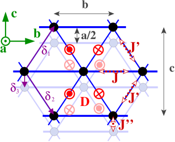
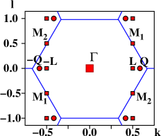
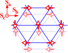
Figure 1: (Color Online) (A) Magnetic sites and exchange couplings of Cs₂CuCl₄ : Even (color) and odd (gray) layers are stacked along the $a$-direction. The signs $\bm{\otimes},\bm{\odot}$ refer to the direction of the DM vector between zig-zag bonds. (B) Reciprocal space plane $(k,l)$, with the projected Brillouin zone, projections of the Brillouin zone center $\Gamma$, the incommensurate (${\bf{Q}},-{\bf{Q}}$) and the commensurate $({\bf{L}},{{\bf{M}}_{1}},{{\bf{M}}_{2}})$ ordering wavevectors indicated. (C) Predicted antiferromagnetic state (Eq. 8) with Bragg peaks at ${{\bf{M}}_{1}}$ and ${{\bf{M}}_{2}}$, showing the orientation of ordered moments projected onto the $a$-$b$ spin plane. Note that here, of necessity, spin coordinates are rotated relative to lattice coordinates.

This spin model can be treated as a lattice gas of hard core bosons. Matsubara01 ; Batyev01 ; Batyev02 ; Gluzman01 ; Nikuni01 In the dilute limit, all quantum effects are incorporated exactly by summing ladder diagrams for the interaction vertices. Beliaev01 ; Abrikosov A Hartree Fock treatment of these effective interactions can be used to obtain the ground state spin structure. We describe further details of the calculation separately for the two cases of longitudinal and transverse magnetic fields.

II.1 Longitudinal Fields

For definiteness, we consider a field in the $c$ direction. We introduce boson creation and annihilation operators $\phi^{\dagger}_{\bf{R}}$ and $\phi^{\phantom{\dagger}}_{\bf{R}}$ and set $S^{c}_{\bf{R}}=\frac{1}{2}-\phi^{\dagger}_{\bf{R}}\phi^{\phantom{\dagger}}_{\bf{R}}$, $S^{+}_{\bf{R}}=S^{a}_{\bf{R}}+iS^{b}_{\bf{R}}=\phi^{\phantom{\dagger}}_{\bf{R}}$ and $S^{-}_{\bf{R}}=S^{a}_{\bf{R}}-iS^{b}_{\bf{R}}=\phi^{\dagger}_{\bf{R}}$. For the spin commutation relations to be satisfied, a hard core constraint on boson number must be imposed by including an on-site repulsion $U$ in the Hamiltonian and taking the limit $U\to\infty$.

The DM interaction is represented by terms cubic in boson creation and annihilation operators, because for this field orientation it couples transverse and longitudinal spin components. Close to the saturation field we are concerned ultimately with an effective description involving only bosons near minima of the dispersion relation generated by the exchange coupling. As argued previously, Veillette01 momentum conservation precludes cubic terms in an effective low energy Hamiltonian. Instead, within second order perturbation theory the DM interactions generate quadratic and quartic couplings between low energy bosons, with magnitude ${\cal O}(D^{2}/J)$. Since $\left|D/J\right|\ll 1$, we neglect altogether the effect of DM interactions in longitudinal fields.

At this point a simplification is possible. In the absence of DM interactions the distinction between odd and even layers disappears. The size of the unit cell in the $a$-direction is halved and that of the Brillouin zone is doubled. We take Fourier transforms using this reduced unit cell. The Hamiltonian (omitting a constant) is

$${\mathcal{H}} =\sum_{\bf{k}}(\epsilon_{\bf{k}}-\mu)\phi^{\dagger}_{\bf{k}}\phi^{\phantom{\dagger}}_{\bf{k}}+\frac{1}{2N}\sum_{{\bf{k}},{\bf{k^{\prime}}},{\bf{q}}}V_{\bf{q}}\phi^{\dagger}_{{\bf{k}}+{\bf{q}}}\phi^{\dagger}_{{\bf{k^{\prime}}}-{\bf{q}}}\phi^{\phantom{\dagger}}_{\bf{k^{\prime}}}\phi^{\phantom{\dagger}}_{\bf{k}},$$ (3)

where $\epsilon_{\bf{k}}=J_{\bf{k}}-J_{\rm min}$ is the boson kinetic energy, $J_{\bf{k}}=1/2\sum_{{\bm{\delta}}}J_{\bm{\delta}}e^{i{\bf{k}}\cdot{\bm{\delta}}}$ is the Fourier transform of the exchange couplings, $\mu=H^{c}_{cr}-H^{c}$ is the boson chemical potential, and $H^{c}_{cr}=J_{{\bf{0}}}-J_{\rm min}$ is the saturation field. The number of lattice sites is $N$ and the interaction vertex is given by $V_{\bf{q}}=2J_{\bf{q}}+2U$. Writing ${\bf{k}}=(h,k,l)$ as shorthand for ${\bf{k}}=2\pi(h/a,k/b,l/c)$, the dispersion relation $\epsilon_{{\bf{k}}}$ has two minima located at the incommensurate wavevectors ${\bf{k}}=\pm{\bf{Q}}=\pm(1,1/2+\epsilon_{0},0)$, where $\sin\pi\epsilon_{0}=J^{\prime}/(2J)$. On reverting to the standard description with two layers in a unit cell, these wavevectors are denoted by ${\bf{Q}}=\pm(0,1/2+\epsilon_{0},0)$ and amplitudes are staggered on the two layers.Coldea2 Note that the degeneracy of the two minima follows from symmetry of the full Hamiltonian Veillette01 and is not lifted by DM interactions.

At this point we can apply standard techniques developed for the interacting Bose gas. Abrikosov With negative $\mu$, the ground state is the boson vacuum. Equivalently, with $H^{c}>H^{c}_{cr}$ the spin system is fully polarized. With positive $\mu$, the boson density is non-zero. Condensation of these bosons at low temperature is equivalent to magnetic order, and we introduce the complex order parameter $\psi_{\bf{q}}=\langle\phi_{\bf{q}}\rangle/\sqrt{N}$. In the dilute regime, the full scattering vertex can be obtained by summing pair interactions in the particle-particle channel. We denote this vertex, for the scattering amplitude of incoming bosons with momenta ${\bf{k}}$ and ${\bf{k^{\prime}}}$ to outgoing states with momenta ${\bf{k}}-{\bf{q}}$ and ${\bf{k^{\prime}}}+{\bf{q}}$, by $\Gamma_{{\bf{q}},{\bf{k}},{\bf{k^{\prime}}}}$. At low density it satisfies the Bethe-Salpeter equation

$$\Gamma_{{\bf{q}},{\bf{k}},{\bf{k^{\prime}}}}\!\!=\!\!V_{\bf{q}}-\frac{1}{N}\sum_{{\bf{q^{\prime}}}}\frac{V_{{\bf{q}}-{\bf{q^{\prime}}}}}{\epsilon_{{\bf{k}}+{\bf{q^{\prime}}}}+\epsilon_{{\bf{k^{\prime}}}-{\bf{q^{\prime}}}}-\epsilon_{{\bf{k}}}-\epsilon_{\bf{k^{\prime}}}}\Gamma_{{\bf{q^{\prime}}},{\bf{k}},{\bf{k^{\prime}}}}\,.$$ (4)

This integral equation can be reduced to a set of linear equations which are readily solved numerically (see Ref. Veillette01, ).

We now proceed to an analysis of the energy of various candidate ground states. This energy can be written in the form of a Landau expansion, in terms of one or more order parameters $\psi_{\bf{q}}$. We first review our earlier results, for behavior immediately below the saturation field. Veillette01 In this regime one expects condensation only at one or both minima of the boson dispersion relation, with wavevectors ${\bf{k}}=\pm{\bf{Q}}$. Allowing for two possible order parameters, the energy per site is

$$E/N =\left(\epsilon_{\bf{Q}}-\mu\right)\left(\left|\psi_{\bf{Q}}\right|^{2}+\left|\psi_{-{\bf{Q}}}\right|^{2}\right)$$

$$+\frac{1}{2}\Gamma_{1}\left(\left|\psi_{\bf{Q}}\right|^{4}+\left|\psi_{-{\bf{Q}}}\right|^{4}\right)+\Gamma_{2}\left|\psi_{\bf{Q}}\right|^{2}\left|\psi_{-{\bf{Q}}}\right|^{2},$$ (5)

with $\Gamma_{1}=\Gamma_{{\bf{0}},{\bf{Q}},{\bf{Q}}}=\Gamma_{{\bf{0}},-{\bf{Q}},-{\bf{Q}}}$ and $\Gamma_{2}=\Gamma_{{\bf{0}},-{\bf{Q}},{\bf{Q}}}+\Gamma_{2{\bf{Q}},-{\bf{Q}},{\bf{Q}}}$. (Here $\epsilon_{\bf{Q}}=0$, but we retain it for future reference). Minimizing the energy with respect to the order parameters, a single component state is favored for $\Gamma_{1}<\Gamma_{2}$. It is the cone state with spin structure $\langle{\bf{S}}_{\bf{R}}\rangle=(\sqrt{n}_{\bf{Q}}\cos(\pm{\bf{Q}}\cdot{\bf{R}}+\alpha),\sqrt{n}_{\bf{Q}}\sin(\pm{\bf{Q}}\cdot{\bf{R}}+\alpha),\frac{1}{2}-n_{\bf{Q}})$, where $n_{\bf{Q}}=(\mu-\epsilon_{\bf{Q}})/\Gamma_{1}$ is the condensate density and $\alpha$ is an arbitrary phase. A two-component state with equal amplitudes for both order parameters is favored for $\Gamma_{1}>\Gamma_{2}$. In this state, ordered moments for a spin fan, with $\langle{\bf{S}}_{\bf{R}}\rangle=(2\sqrt{n}_{\bf{Q}}\cos({\bf{Q}}\cdot{\bf{R}}+\alpha)\cos(\beta),2\sqrt{n}_{\bf{Q}}\cos({\bf{Q}}\cdot{\bf{R}}+\alpha)\sin(\beta),1/2-4n_{\bf{Q}}\cos^{2}({\bf{Q}}\cdot{\bf{R}}+\alpha))$, where $n_{\bf{Q}}=n_{-{\bf{Q}}}=(\mu-\epsilon_{\bf{Q}})/(\Gamma_{1}+\Gamma_{2})$ and $\alpha,\beta$ are arbitrary phases. A numerical evaluation of Eq. 4 yields $\Gamma_{1}=3.79J$ and $\Gamma_{2}=4.67J$, so the cone state is selected. It has energy per site ${E}/{N}=-{(\epsilon_{\bf{Q}}-\mu)^{2}}/{2\Gamma_{1}}$.

At this stage, we have established that the ground state for $\mu=0^{+}$ is the cone state. Next we examine whether there is a transition to a commensurate ground state at a larger value of $\mu$. A first possible commensurate state is one with order at the wavevector ${\bf{L}}=(1,1/2,0)$, using our description with a single layer per unit cell (equivalent to $(0,1/2,0)$ in the standard notation with two layers per unit cell). This is a natural choice because ${\bf{L}}$ lies close to ${\bf{Q}}$, and because the wavevector of incommensurate order is known to move towards ${\bf{L}}$ with increasing $\mu$.Veillette01 We find nevertheless, repeating the calculations we have outlined, but with ${\bf{L}}$ in place of ${\bf{Q}}$ and with $\epsilon_{{\bf{L}}}>0$, that the commensurate spin cone and spin fan states are higher in energy than the incommensurate states, as shown in Fig. 2.

An second possible commensurate state is one with condensates at the wavevectors ${{\bf{M}}_{1}}=\left(1,\frac{1}{2},\frac{1}{2}\right)$ and ${{\bf{M}}_{2}}=\left(1,-\frac{1}{2},\frac{1}{2}\right)$, in our notation (or $\left(0,\frac{1}{2},\frac{1}{2}\right)$ and $\left(0,-\frac{1}{2},\frac{1}{2}\right)$ in the standard notation), and it is in fact at those positions that magnetic Bragg peaks are observed experimentally.Unknown01 The difference ${\bf{\Delta M}}={{\bf{M}}_{2}}-{{\bf{M}}_{1}}$ is half a reciprocal lattice vector so that umklapp scattering between the condensates is allowed and may reduce the energy of the state. We obtain an energy per site

$$E/N =\left(\epsilon_{{{\bf{M}}_{1}}}-\mu\right)\left(\left|\psi_{{\bf{M}}_{1}}\right|^{2}+\left|\psi_{{\bf{M}}_{2}}\right|^{2}\right)$$

$$+\frac{1}{2}\Gamma_{A}\left(\left|\psi_{{\bf{M}}_{1}}\right|^{4}+\left|\psi_{{\bf{M}}_{2}}\right|^{4}\right)+\Gamma_{B}\left|\psi_{{\bf{M}}_{2}}\right|^{2}\left|\psi_{{\bf{M}}_{1}}\right|^{2}$$

$$+\frac{1}{2}\Gamma_{C}\left(\psi^{\ast 2}_{{\bf{M}}_{1}}\psi^{2}_{{\bf{M}}_{2}}+c.c.\right),$$ (6)

where $\Gamma_{A}=\Gamma_{{\bf{0}},{{\bf{M}}_{1}},{{\bf{M}}_{1}}}=\Gamma_{{\bf{0}},{{\bf{M}}_{2}},{{\bf{M}}_{2}}}=3.36J$, $\Gamma_{B}=\Gamma_{{\bf{0}},{{\bf{M}}_{1}},{{\bf{M}}_{2}}}+\Gamma_{{\bf{\Delta M}},{{\bf{M}}_{1}},{{\bf{M}}_{2}}}=0$ and $\Gamma_{C}=\Gamma_{{\bf{\Delta M}},{{\bf{M}}_{1}},{{\bf{M}}_{1}}}=1.30J$. The amplitude $\Gamma_{B}$ is zero because the denominator in Eq. (4), $\epsilon_{{\bf{k}}+{\bf{q^{\prime}}}}+\epsilon_{{\bf{k^{\prime}}}-{\bf{q^{\prime}}}}-\epsilon_{{\bf{k}}}-\epsilon_{\bf{k^{\prime}}}$, depends on only two components of ${\bf{q^{\prime}}}$ for ${\bf{k}}={{\bf{M}}_{1}}$ and ${\bf{k^{\prime}}}={{\bf{M}}_{2}}$. This leads to vanishing interactions, as is familiar from the example of the two dimensional Bose gas.Fisher01

The energy of this commensurate state is minimized by setting $\psi_{{{\bf{M}}_{1}}}=\pm i\psi_{{{\bf{M}}_{2}}}$, giving

$$\frac{E}{N}=-\frac{\left(\epsilon_{{{\bf{M}}_{1}}}-\mu\right)^{2}}{\Gamma_{A}+\Gamma_{B}-\Gamma_{C}}\,.$$ (7)

We find that it is lower than the energy of the incommensurate cone state for fields smaller than $H^{c}_{T1}=0.958H^{c}_{cr}$: see Fig. 2. The proximity of $H^{c}_{T1}$ to $H^{c}_{cr}$ justifies our use of the low density approximation. The components of the ordered moment in this commensurate state are

$$\langle S^{a}_{\bf{R}}\rangle =\sqrt{n_{c}}\left(\cos({{\bf{M}}_{1}}\cdot{\bf{R}}+\alpha)\pm\sin({{\bf{M}}_{2}}\cdot{\bf{R}}+\alpha)\right),$$

$$\langle S^{b}_{\bf{R}}\rangle =\sqrt{n_{c}}\left(\sin({{\bf{M}}_{1}}\cdot{\bf{R}}+\alpha)\mp\cos({{\bf{M}}_{2}}\cdot{\bf{R}}+\alpha)\right),$$

$$\langle S^{c}_{\bf{R}}\rangle =\frac{1}{2}-2n_{c}\,,$$ (8)

where $n_{c}=({\mu-\epsilon_{{\bf{M}}_{1}}})/({\Gamma_{A}+\Gamma_{B}-\Gamma_{C}})$ and $\alpha$ is an arbitrary phase. This structure is illustrated in Fig. 1. In this commensurate state neighboring spins are antiferromagnetically aligned along the chains and in adjacent layers, but perpendicular in adjacent chains. The $\pm$ sign in Eq. 8 reflects the two distinct ways to arrange this perpendicular orientation. The experimental phase diagram in longitudinal field is summarized in Fig. 2, together with the theoretical results obtained here for behavior close to the saturation field, and earlier ones for large $S$.

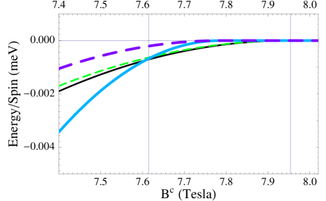
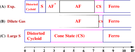
Figure 2: (Color Online) Ground states in longitudinal fields. Top: Energies of states considered [Eqns. (5) and (6)] as a function of longitudinal magnetic field $B^{c}$, computed using $g^{c}=2.30$.Gfactor The thin, thick, short-dashed and long-dashed lines represent, respectively: the incommensurate cone state; the commensurate state with condensates at ${{\bf{M}}_{1}}$ and ${{\bf{M}}_{2}}$; the incommensurate spin-fan; and the commensurate state with condensate at ${\bf{k}}={\bf{L}}$. The incommensurate cone state is the ground state for $B^{c}_{T1}<B^{c}<B^{c}_{cr}$, with $B^{c}_{cr}=7.95T$ and $B^{c}_{T1}=7.615T$. The commensurate state at ${{\bf{M}}_{1}}$ and ${{\bf{M}}_{2}}$ is the ground state for $B^{c}<B^{c}_{T1}$. Bottom: Phase diagram in longitudinal fields: (A) from experiment; (B) from dilute Bose gas calculation; (C) from large S-expansionVeillette01 . Here $S$ denotes an incommensurate phase, and $AF$ and $AF^{*}$ indicate commensurate phases, observed experimentally to have magnetic Bragg peaks at ${{\bf{M}}_{1}}$ and ${{\bf{M}}_{2}}$.

II.2 Transverse fields

In a transverse field, the DM vector is parallel to the field direction and so the DM interaction is quadratic in boson creation and annihilation operators. Using the standard unit cell containing two layers, and introducing separate species of bosons for the even and odd layers, the quadratic Hamiltonian isColdea2

$${\mathcal{H}}\! =\!\sum_{\bf{k}}\!\begin{bmatrix}\phi^{\dagger}_{e{\bf{k}}}\!&\!\phi^{\dagger}_{o{\bf{k}}}\end{bmatrix}\begin{bmatrix}\Omega_{\bf{k}}\!-\!J^{\prime\prime}\!+\!D_{\bf{k}}\!\!\!&\!J^{\prime\prime}_{-{\bf{k}}}\!\\ \!J^{\prime\prime}_{\bf{k}}\!&\!\!\!\Omega_{\bf{k}}\!-\!J^{\prime\prime}\!-\!D_{\bf{k}}\\ \end{bmatrix}\begin{bmatrix}\phi^{\phantom{\dagger}}_{e{\bf{k}}}\\ \phi^{\phantom{\dagger}}_{o{\bf{k}}}\end{bmatrix},$$

where $\Omega_{\bf{k}}=J_{\bf{k}}-J_{\bf{0}}+H^{a}$, evaluated with $J^{\prime\prime}=0$, $D_{\bf{k}}=-D\left(\sin({\bf{k}}\cdot{\bm{\delta}}_{1})+\sin({\bf{k}}\cdot{\bm{\delta}}_{2})\right)$ and $J^{\prime\prime}_{\bf{k}}=J^{\prime\prime}\cos({\bf{k}}\cdot{\bm{\delta}}_{3})$. Diagonalization of this Hamiltonian yields a dispersion relation with two branches $\epsilon^{\pm}_{{\bf{k}}}$. Because of DM interactions, the branches lack inversion symmetry: $\epsilon^{\pm}_{\bf{k}}\neq\epsilon^{\pm}_{-{\bf{k}}}$. Coldea4 Below the saturation field, order appears at the incommensurate wavevectors that minimize $\epsilon^{+}_{\bf{k}}$ and $\epsilon^{-}_{\bf{k}}$.Coldea2 ; Veillette01 ; Coldea4 It is likely that any further transition to a commensurate phase will be disfavored by the reduced symmetry of the dispersion relation in a transverse field. To test this, we have carried out calculations of the energies of commensurate states in a transverse field analogous to the ones described for a longitudinal field. To simplify these calculations, we have treated a model in which the DM vector is not staggered between layers, so that the unit cell contains only a single layer, rather than two. (See Ref. Coldea4, for an alternative approach.) A similar calculation to the one performed in longitudinal fields reveals that the incommensurate state is lowest in energy in transverse fields (see Fig. 3) in agreement with experimental data and the $1/S$ expansion.

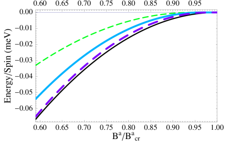
Figure 3: (Color Online) Ground state in transverse fields. Energies of various states as a function of transverse magnetic field $B^{a}$ (normalized with respect to the critical field). The thin, thick, short-dashed and long-dashed lines represent, respectively: the incommensurate cone state; the commensurate state with condensates at ${{\bf{M}}_{1}}$ and ${{\bf{M}}_{2}}$; the incommensurate spin-fan; and the commensurate state with condensate at ${\bf{k}}={\bf{L}}$.

III Summary

In summary, we have studied the magnetic ground states of Cs₂CuCl₄ in the vicinity of the saturation field by treating reversed spins as a dilute Bose gas. In a transverse field we find only an incommensurate ground state , in agreement with experiment and calculations based on the $1/S$ expansion. By contrast, in a longitudinal field there is a transition between an incommensurate state close to the saturation field and a commensurate state at lower field. We propose that this commensurate state is the one recently observed in neutron diffraction.Unknown01

References

- (1) R. Coldea, D. A. Tennant, R. A. Cowley, D. F. McMorrow, B. Dorner, and Z. Tylczynski, J. Phys.: Condens. Matter 8, 7473 (1996).
- (2) R. Coldea, D. A. Tennant, A. M. Tsvelik, and Z. Tylczynski, Phys. Rev. Lett. 86, 1335 (2001).
- (3) R. Coldea, D. A. Tennant, K. Habicht, P. Smeibidl, C. Wolters, and Z. Tylczynski, Phys. Rev. Lett. 88, 137203 (2002).
- (4) R. Coldea, D. A. Tennant, and Z. Tylczynski, Phys. Rev. B 68, 134424 (2003).
- (5) T. Radu, H. Wilhelm, V. Yushankhai, D. Kovrizhin, R. Coldea, Z. Tylczynski, T. Luehmann, and F. Steglich, Phys. Rev. Lett. 95, 127202 (2005).
- (6) R. Coldea and D.A. Tennant (private communication).
- (7) P.W. Anderson, Mater. Res. Bull. 8, 153 (1973).
- (8) M. Bocquet, F. H. L. Essler, A. M. Tsvelik, and A. O. Gogolin, Phys. Rev. B 64, 094425 (2001).
- (9) C. H. Chung, J. B. Marston, and R. H. McKenzie, J. Phys.: Condens. Matter 13, 5159 (2001).
- (10) C. -H. Chung, K. Voelker, and Y. B. Kim, Phys. Rev. B 68, 094412 (2003).
- (11) S. V. Isakov, T. Senthil, and Y. B. Kim, Phys. Rev. B 72, 174417 (2005).
- (12) M. Y. Veillette, A. J. A. James, and F. H. L. Essler, Phys. Rev. B 72, 134429 (2005).
- (13) J. Alicea, O. I. Motrunich, and M. P. A. Fisher, (unpublished), cond-mat/0508536.
- (14) W. Zheng, J. O. Fjaerestad, R. R. P. Singh, R. H. Mackenzie, and R. Coldea, (unpublished), cond-mat/0506400.
- (15) M. Y. Veillette, J. T. Chalker, and R. Coldea, Phys. Rev. B 71, 214426 (2005).
- (16) D. L. Kovrizhin, V. Yushankai, and L. Siurakshina, (unpublished) cond-mat/0509552.
- (17) Experimentally, there appears to be a weak anisotropy within the easy plane, which is not included in the model Hamiltonian, and which we ignore in this paper.
- (18) E. G. Batyev and L. S. Braginskii, Zh. Eksp. Teor. Fiz. 87, 1361 (1984) [Sov. Phys. JETP 60, 781 (1984)].
- (19) E. G. Batyev, Zh. Eksp. Teor. Fiz. 89, 308 (1985) [ Sov. Phys. JETP 62, 173 (1985)].
- (20) S. Gluzman, Z. Phys. B: Condens. Matter 90, 313, (1993).
- (21) T. Nikuni and H. Shiba, J. Phys. Soc. Jpn. 64, 3471 (1995).
- (22) T. Matsubara and H. Matsuda, Prog. Theor. Phys. 16, 569 (1956).
- (23) A. A. Abrikosov, L. P. Gorkov, and I. E. Dzyaloshinskii in Methods of Quantum Field Theory In Statistical Physics, (Dover, New York, 1975).
- (24) S. T. Beliaev, Zh. Eksp. Teor. Fiz. 34, 417 (1958) [Sov. Phys. JETP 7, 289 (1958)]. S. T. Beliaev, Zh. Eksp. Teor. Fiz. 34, 433 (1958) [Sov. Phys. JETP 7, 299 (1958)].
- (25) D. S. Fisher and P. C. Hohenberg, Phys. Rev. B 37, 4936 (1988).
- (26) S. Bailleul, J. Holsa, and P. Porcher, Eur. J. Solid State Inorg. Chem. 31, 432 (1994).