Self-trapping of Bose-Einstein condensates in optical lattices

Abstract

The self-trapping phenomenon of Bose-Einstein condensates (BECs) in optical lattices is studied extensively by numerically solving the Gross-Pitaevskii equation. Our numerical results not only reproduce the phenomenon that was observed in a recent experiment [Anker et al., Phys. Rev. Lett. 94 (2005)020403], but also find that the self-trapping breaks down at long evolution times, that is, the self-trapping in optical lattices is only temporary. The analysis of our numerical results shows that the self-trapping in optical lattices is related to the self-trapping of BECs in a double-well potential. A possible mechanism of the formation of steep edges in the wave packet evolution is explored in terms of the dynamics of relative phases between neighboring wells.

I Introduction

Progress in recent years has shown that a Bose-Einstein condensate(BEC) in an optical lattice is a fascinating periodic system, where the physics can be as rich as in fermionic periodic systems, the main subject of condensed-matter physics. In such a bosonic system, people have observed well-known and long predicted phenomena, such as Bloch oscillations Morsch et al. (2001) and the quantum phase transition between superfluid and Mott-insulatorGreiner et al. (2002). More importantly, there are new phenomena that have been either observed or predicted in this system, for example, nonlinear Landau-Zener tunneling between Bloch bands Jona-Lasinio et al. (2003); Wu and Niu (2000) and the strongly inhibited transport of one dimensional BEC in an optical latticeFertig et al. (2005).

Another intriguing phenomenon, self-trapping, was recently observed experimentally in this systemAnker et al. (2005). In this experiment, a BEC with repulsive interaction was first prepared in a dipole trap. By adiabatically ramping up an optical lattice, the BEC was essentially transformed into a Bloch state at the center of the Brillouin zone. With the optical lattice always on, the BEC was then released into a trap that serves as a one dimensional waveguide. The evolution of the BEC cloud inside the combined potential was studied by taking absorption images. When the number of atoms in the BEC is small, say around 2000, the BEC wave packet was found to expand continuously (which is expected). However, when the number of atoms was increased to about 5000, it was observed that the BEC cloud stops to expand after initially expanding for about 35ms (see Fig.1). This is quite counter-intuitive. Without interaction, a wave packet with a narrow distribution in the Brillouin zone expands continuously inside a periodic potential. One would certainly expect that with a repulsive interaction between atoms the BEC cloud spread faster. This experiment showed the contrary: if the cloud is dense enough, it self-traps and stops spreading.

Figure 1: The width of the BEC wave packet as a function of time for $N=2000$ and $N=5000$. $N$ is the number of atoms in the BEC. The solid lines are our numerical results while the circles and squares are experimental data from Ref.Anker et al. (2005).

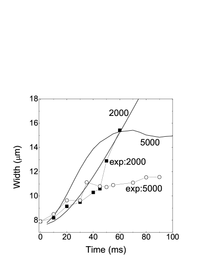
To understand this intriguing phenomenon, we have carried out extensive numerical study of this system with the one-dimensional(1D) Gross-Pitaevskii equation. Our results match quite well with the experimental data as shown in Fig.1. When the atom number $N$ in the BEC is 2000, the agreement between our numerical results and the experiment is excellent; when $N=5000$, our results are about 40% larger than the experimental data. The discrepancy in the latter case is likely caused by the higher density: with higher density the lateral motion of the BEC cloud may become more relevant to the longitudinal expansion; however, the lateral motion is completely ignored in our numerical study as we use the 1D Gross-Pitaevskii equation.

Figure 2: The width of the BEC wave packet as a function of time for $N=1000,2000,3000,4000,5000,7000$, and $50000$.

Very interestingly, we find that the self-trapping is temporary. After a sufficiently long evolution time, the self-trapping breaks down and the wave packet starts to expand again as seen in Fig.2. Since the break-down time is much longer than the observation used in the current experimentAnker et al. (2005), these results need to be verified in future experiments. This breakdown of self-trapping is likely caused by the leakage of atoms at the outmost wells, or as we shall call it the dripping effect. Furthermore, our numerical results show that the steep edges do not necessarily lead to the self-trapping and always appear in the wave packet evolution, independent of its denseness of the BEC cloud. This is different from Ref.Anker et al. (2005), where it was pointed out that the steep edges appearing at the two sides of the wave packet are crucial for the appearance of the self-trapping. The wave packet evolution in the quasi-momentum space is also studied. We find that the wave packet localizes largely near the center of the Brillouin zone; no major interesting features can be identified during the evolution.

Besides, we have analyzed our numerical results in detail, in particular, in terms of the relative atom number difference and the relative phase difference between neighboring wells. With such an analysis, we have confirmed the previous studyAnker et al. (2005) that the self-trapping observed in optical lattices is closely related to the self-trapping of a BEC in the double-well potential Milburn et al. (1997); Smerzi et al. (1997); Albiez et al. (2005). From this analysis, we have also explored a possible mechanism of the formation of steep edges.

Our paper is organized as follows. We shall first present a brief description of our numerical method. We then describe how the wave packets evolve in our numerical simulation. Afterwards, we analyze our numerical results in an attempt to understand our numerical results. The analysis is done from the angle of a BEC in a double-well potential. Summary and some discussion are given at the end.

II Numerical method

To model the experiment, we use the following Gross-Pitaevskii(GP) equation

$$i\hbar{\partial\over\partial t}\psi(\bm{r},t)=-{\hbar^{2}\over 2m}\nabla^{2}\psi(\bm{r},t)+V_{0}\cos(2k_{L}x)\psi(\bm{r},t)+$$

$$\leavevmode\nobreak\ \leavevmode\nobreak\ \leavevmode\nobreak\ \leavevmode\nobreak\ \leavevmode\nobreak\ \leavevmode\nobreak\ +V_{wg}(\bm{r})\psi(\bm{r},t)+\frac{4\pi\hbar^{2}a_{s}}{m}|\psi(\bm{r},t)|^{2}\psi(\bm{r},t)\,,$$ (1)

where $m$ is the atomic mass, $a_{s}$ is the $s$-wave scattering length, $k_{L}$ is the wavelength of the laser that generates the optical lattice, and $V_{wg}(\bm{r})$ describes the waveguide potential. Due to the tight confinement perpendicular to the optical lattice from the waveguide potential, the dynamics of this system is largely one-dimensional. This allows us to integrate out the two perpendicular directions and reduce the above GP equation to

$$i{\partial\psi(x,t)\over\partial t} = -{1\over 2}\nabla^{2}\psi(x,t)+V\cos(x)\psi(x,t)+$$ (2)

$$+ {1\over 2}\omega x^{2}\psi(x,t)+g|\psi(x,t)|^{2}\psi(x,t)\,,$$

were we have made the equation dimensionless. In doing so, we have $x$ in units of $1/2k_{L}$ and $t$ in $m/4\hbar k_{L}^{2}$. The strength of the optical lattice is given $V=V_{0}/16E_{r}$ with $E_{r}=\hbar^{2}k_{L}^{2}/2m$ being the recoil energy. For the nonlinear interaction, we have

$$g={\pi a_{s}m\omega_{\bot}N\over\surd 2\pi\hbar k_{L}}\,,$$ (3)

where $N$ the total number of the BEC in the harmonic trap and $\omega_{\bot}$ is the transverse trapping frequency of the waveguide. The other frequency $\omega$ is so chosen that the initial rms-width of BEC wave packet is $7.6\mu$m as in the experimentsAnker et al. (2005). This width corresponds to about 100 wells occupied. The wave function $\psi$ is normalized to one. In our numerical simulation, we use the following values from the experimentAnker et al. (2005), $\lambda=2\pi/k_{L}=783$nm, $V_{0}=10E_{r}$, and $\omega_{\bot}=2\pi\times 230$Hz.

To simulate the experiment, we prepare our initial wave function $\psi$ to be the ground state in the combined potential of $V\cos(x)+{1\over 2}\omega x^{2}$. This is achieved by integrating Eq.(2) with imaginary time. In the experiment, the waveguide potential also has a longitudinal trapping frequency at $\omega_{\parallel}=2\pi$Hz, which is very weak and can be ignored. Therefore, after obtaining the initial wave function, we completely remove the longitudinal trapping and let the wave function evolve according to the following equation

$$i{\partial\psi\over\partial t}=-{1\over 2}\nabla^{2}\psi+V\cos(x)\psi+g|\psi|^{2}\psi\,.$$ (4)

The evolutions are subsequently recorded and analyzed.

III Wave packet evolution

With the above method, we have computed the evolution of the wave packets for different numbers of atoms in the BEC. As indicated in Eq.(3), the number of atoms in the BEC translates into the nonlinear parameter: larger the atom number $N$ stronger the nonlinearity (or the repulsive interaction). Fig.2 illustrates how the width of a wave packet evolves for different atom numbers.

Figure 3: Time evolution of the wave packet density for $N=5000$.

It is clear from this figure that, when the BEC is dilute and has small atom numbers, $N\lesssim 2000$, the wave packet expands continuously without stopping as one may have expected. Also as expected, in this range, when the number of atoms increases, the expansion becomes faster. The evolution becomes very different when the BEC is denser. We see in Fig.2 that for $N=3000$, the wave packet expansion slows down around 70ms and becomes slower than the wave packet for $N=2000$ around 85ms. This means that we have slower expansion for a denser cloud of repulsive interaction, a rather counter-intuitive result. As the cloud gets denser with more atoms, the expansion slows down further. Around $N=5000$, there even appears a plateau where the cloud stops expanding and becomes self-trapped as observed in the experimentAnker et al. (2005). Fig.2 illustrates a key point in this intriguing self-trapping phenomenon: it does not happen in a sudden and it is a gradual process. Before it happens, the wave packet expansion already slows down for higher enough densities.

What is more interesting is that, in our numerical simulation, the wave packet continues to expand after pausing for 30-40ms. For $N=5000$, the expansion re-starts at $\sim 85$ms, just beyond the longest observation time in Ref.Anker et al. (2005). Therefore, this continued expansion awaits for verification in future experiments. Nevertheless, the counter-intuitive phenomenon, denser clouds expand slower, persists even after the expansion re-starts as we can see in Fig.2. In the next section, we shall offer an explanation of this self-trapping phenomenon and explain why it is only temporary. Just out of curiosity, we also computed the case of very large atom number $N=50,000$; we find that the wave packet is almost never seen to spread. This is likely due to that the self-trapping lasts too long to be observed in our numerical simulations.

Figure 4: Time evolution of the wave packet density for $N=2000$ before $t=80$ms.

Figure 5: Time evolution of the wave packet density for $N=2000$ after $t=80$ms.

Shown in Fig.3 are some snapshots of the time evolution of the wave packet for $N=5000$. Around $t=30$ms, steep edges are seen growing pronounced on both sides of the wave packet. Moreover, in the subsequent evolution, the positions of the steep edges do not move out any further. When compared with Fig.1, it is clear that this appearance of the steep edges coincides with the non-spreading of the wave packet. Therefore, it seems that the steep edges seen in Fig.3 signal the emergence of the self-trapping as suggested in Ref.Anker et al. (2005). The following results indicate otherwise.

Fig.4 shows the time evolution of the wave packet for $N=2000$. Before 80ms (about the longest experimental observation time in Ref.Anker et al. (2005)), there are no steep edges. However, around 85ms, the steep edges begin to appear and grow more and more pronounced as the evolution goes on. What is different from $N=5000$ is that these steep edges continue to move out during the time evolution and the width of the wave packet also grows with time. There is no self-trapping. This clearly shows that the steep edges do not necessarily lead to the self-trapping of the wave packet.

We have also computed how the wave packet evolves in the quasi-momentum space. To achieve this, we expand the wave packet in terms of the Bloch waves belonging to the lowest Bloch band of the linear system with the periodic potential $\cos x$. The results are plotted in Fig.6, where we do not see a large population around $k=1/4$. Therefore, the link between the formation of steep edges and the population at $k=1/4$ believed in Ref.Anker et al. (2005) is not established here.

Figure 6: Time evolution of the wave packet in the quasi-momentum space for $N=5000$.

Figure 7: The dynamic of nonlinear energy of each atom for $N=2000$ (dashed)and $N=5000$ (solid).

Another quantity that can be used to characterize the self-trapping phenomenon is the nonlinear energy of the BEC, which is given by $\int\frac{g}{2}|\psi(x,t)|^{4}dx$. If the wave packet expands continuously, the nonlinear energy should decrease with the expansion. If there is self-trapping, i.e., the wave packet stops to grow, then the nonlinear energy should remain largely constant. Indeed, this is the case as shown in Fig.7, where the nonlinear energy does not decrease and only fluctuates slightly when the self-trapping occurs.

IV relationship to the self-trapping in a double-well

It has been known for a while that the self-trapping also occurs for a BEC in a double-well potential Milburn et al. (1997); Smerzi et al. (1997); WangGF2005 ; Albiez et al. (2005). It is then natural to ask whether the self-trappings in these two different systems are related to each other. Our analysis shows that these two are closely related.

Figure 8: The values of $\xi$ and $s$ of a wave packet at $t=40$ms for $N=5000$. (a) The values of $\xi$ at different wells (The $\xi$ at the $n$th well is for the double wells composed of the $n$th and $n+1$th wells. (b) Phase diagram (or distribution) of $\xi$ and $s$ for this wave packet. The self-trapping occurs at $t=40$ms.

This was already noticed in Ref.Anker et al. (2005) based on numerical results with a tight-binding approximation of the GP equation; here we offer a more detailed analysis with numerical results with the full GP equation. Our analysis leads to a possible explanation why the self-trapping observed in the optical lattice is only temporary and how the steep edges form. For the sake of self-containment and introducing new parameters, we briefly review the self-trapping in the double-well situation.

Figure 9: The values of $\xi$ and $s$ of a wave packet at $t=110$ms for $N=2000$. (a) The values of $\xi$ at different wells (The $\xi$ at the $n$th well is for the double wells composed of the $n$th and $n+1$th wells. (b) Phase diagram (or distribution) of $\xi$ and $s$ for this wave packet. The time 110ms is when the steep edges start to appear.

The Hamiltonian governing the dynamics of a BEC in a double-well potential can be written asMilburn et al. (1997); Smerzi et al. (1997); WangGF2005 ,

$$H_{classical}=-{c\over 2}s^{2}+v\sqrt{1-s^{2}}\cos\theta,$$ (5)

where $\theta=\theta_{b}-\theta_{a}$ is the relative phase between the two wells $a$ and $b$ while $s$ is the fractional population difference $s=(N_{b}-N_{a})/(N_{a}+N_{b})$ with $N_{a}$ and $N_{b}$ being the number of atoms in wells $a$ and $b$, respectively. Previous studies Milburn et al. (1997); Smerzi et al. (1997); WangGF2005 show that there are two types of self-trapping in this system, depending on the ratio $\xi=c/v$ and the population difference $s$. They are: (1) If $1<\xi<2$ and the relative phase $\theta$ is around $\pi$, then the self-trapping occurs when $s>0.5$. This is called ’oscillation type’ self-trapping. (2) If $\xi>2$ and $s>0.5$, another type of self-trapping emerges with the relative phase $\theta$ between the two wells increasing with time. Therefore, it is called ’running phase type’ self-trapping.

Any pair of neighboring wells in the optical lattice can be viewed as a double-well. To establish the link between the self-trappings in the optical lattice and the double-well, we need to compute $\xi$ and $s$ for each pair of the neighboring wells in the optical lattice for a given wave packet. The details of how $\xi$ is computed for neighboring wells in an optical lattice can be found in Appendix A.

Figure 10: Phase diagrams (or distributions) of $s$ and $\xi$ for wave packets at different evolution times. $N=5000$.

Fig.8 shows one set of such calculations for a wave packet with $N=5000$ at $t=40$ms, which is the time when the self-trapping happens. It is clear from Fig.8(a) that there are four pairs of double-wells whose $\xi$ and $s$ satisfy the condition for the “running phase type” self-trapping in the double-well system. Furthermore, two of these four pairs, marked by A and B in Fig.8, are located right at the two edges of the wave packet. (The other two are just nearby, for clarity we do not mark them.) It seems to suggest that these two self-trapped pairs of double-wells serve as two dams stopping the flow of atoms to the outside. Therefore, the self-trapping in the optical lattice appears just alternative manifestation of the self-trapping in the double-well system.

To firmly establish such a link, we have also examined the case $N=2000$, where there is no self-trapping. Fig.9 shows the values $s$ and $\xi$ for the wave packet with $N=2000$ at $t=110$ms. This is the time when the steep edges have already developed. We see from the figure that all the values of $\xi$ are smaller than one: the self-trapping conditions of the double-well system are not satisfied by any pair of neighboring wells in the optical lattice.

The above analysis leads to the following conclusion: when there is self-trapping in the optical lattice, there are neighboring wells that satisfy the self-trapping condition of the double-well system; when there is no self-trapping in the optical lattice, any pair of the neighboring wells in the lattice does not satisfy the double-well self-trapping condition. So established is a solid link between these two self-trapping phenomena. One intuitive way of understanding of this link is such. Once the self-trapping happens in some pairs of neighboring wells around the edges of a wave packet, these self-trapped double-wells, behaving like “dams”, stop the tunneling of atoms towards outside, causing the non-spreading of the wave packet. In Fig.10 we have plotted a series of “phase diagrams”, where the distribution of the $s$-$\xi$ pairs is shown. The square region bounded by the dashed line in each panel is the area where the self-trapping conditions are satisfied. We can see clearly from this figure that the self-trapping happens from about $t=40$ms to 80ms for $N=5000$. We have also checked the cases of $N=7000$ and $N=50,000$ and reached the same conclusion.

This link not only explains why the self-trapping occurs in the optical lattice but also offers a possible mechanism why the self-trapping is temporarily lived. At the outmost wells, the density of the BEC is very low and the self-trapping conditions of the double-well system can never be satisfied. As a result, the atoms will tunnel towards outside. The amount of atoms tunneling out is very small and has not much effect on the evolution of the whole cloud. However, for long evolution times, this small amount of “dripping” can lead to the significant decreasing of atom numbers in the wells, thus destroy the self-trapping. This is similar to that small cracks can cause the collapse of a dam in a long time.

Based on the link between these two self-trappings, it is also possible to understand why the BEC cloud expands slower around $N=3000$ than $N=2000$ seen in Fig.2. As one can imagine, when the cloud density increases, some pairs of the wells will get close to satisfy these self-trapping conditions and eventually satisfy them. For the medium densities,e.g., $N=3000$ there should be a few pairs of the wells that satisfy the conditions just barely. As a result, the self-trapping conditions can be easily or quickly destroyed by the “dripping” effect mentioned above. However, as the cloud expands, the self-trapping conditions can again be satisfied by some pairs of well further inside and then destroyed again. This on-and-off process can dramatically lead to slowing down of the cloud expansion. What is a pity is that this straightforward picture is hard to be corrobarated by our numerical computation because the values $s$ and $\xi$ for neighboring wells can only be computed approximately. Alternative methods may be needed to verify this picture.

Figure 11: The evolution of relative phases for each pair of neighboring wells in the optical lattice. $N=2000$.

V Steep edges

Figure 12: The evolution of relative phases for each pair of neighboring wells in the optical lattice. $N=5000$.

Figure 13: The evolution of relative populations $s$ for each pair of neighboring wells in the optical lattice. $N=2000$.

Figure 14: The evolution of relative populations $s$ for each pair of neighboring wells in the optical lattice. $N=5000$.

There is a mystery in the wave packet evolution yet to be explained, that is, the appearance of steep edges. Our following analysis shows that the formation of steep edges can also be understood in terms of the BEC dynamics in the double-well system. For future convenience, we write down the dynamics in the double-well system

$$\dot{s} = v\sqrt{1-s^{2}}\sin\theta,$$ (6)

$$\dot{\theta} = -cs-{vs\cos\theta\over\sqrt{1-s^{2}}},$$ (7)

which are derived from the Hamiltonian in Eq.(5).

In Fig.11, we have plotted how the relative phases $\theta$ evolve with time for $N=2000$. In our calculation, the relative phase $\theta$ is defined as the phase difference between the middle points in two neighboring wells. Initially, the relative phase is zero for every pair of double-wells in the optical lattice as indicated by a horizontal line. As the evolution goes on, the line of relative phase begins to incline with an increasing slope. The tendency stops when the two end points of the line reach $\pm\pi/2$, respectively. This is around $t=80$ms, right when the steep edges appear. As shown in Fig.12, the situation is similar for $N=5000$. We also observe from Figs.13&14 that the relative populations in the middle of the wave packet remain largely zero before the appearance of steep edges.

According to Eq.(6), at $\theta\sim\pi/2$ and $s\sim 0$, the tunneling or transfer of atoms between these neighboring wells is the largest. This means that there are more atoms flowing into some particular wells than going out, thus generating steep edges. We notice that right after the appearance of the steep edges. both $s$ and $\theta$ become rather “random”. This is likely due to the complicated dynamics caused by steep edges.

VI conclusion

With the GP equation, we have studied the wave packet dynamic of a BEC in a one-dimensional optical lattices. We find an intriguing self-trapping phenomenon in the expansion of the wave packet, agreeing with a recent experimentAnker et al. (2005). Moreover, we find that the self-trapping is only temporary and the wave packet continues to grow at long evolution times that are beyond the current experimentAnker et al. (2005). The analysis of our numerical results shows that the self-trapping in the optical lattice is closely related to the self-trapping found in the system of a BEC in a double-well potential. We also showed that the steep edges appearing the wave packet evolution do not necessarily lead to self-trapping and they can also be understood in terms of the dynamics in the double-well systems.

Appendix A Computation of $\xi$ in optical lattices

We choose one well and its neighbor as a double well trap. The GP equation is as Eq. (4) except the potential is replaced by $V(x)=V\cos(x)$ for $|x|<2\pi$ and $V(x)=V$ for $|x|>2\pi$. Then we write the wave function as a two-mode wave function: $\phi=au_{1}(x)+bu_{2}(x)$ and let $|a|^{2}=N_{a}/(N_{a}+N_{b})$ and $|b|^{2}=N_{b}/(N_{a}+N_{b})$ ($N_{a}$ is the particle number in well a and $N_{b}$ the particle number in well b). Plugging the double mode wave function into the GP equation with potential $V(x)$ and using the tight-binding approximation, we obtain the effective Hamiltonian:

$$H_{eff}=-c/2(|a|^{2}-|b|^{2})^{2}+v(a^{*}b+ab^{*}),$$ (8)

where the parameter $c=(N_{a}+N_{b})Ng\int|u_{1}(x)|^{4}dx$ and $v=N\int(-{1\over 2}\triangledown u_{1}^{*}(x)\triangledown u_{2}(x)+V^{\prime}(x)u_{1}^{*}(x)u_{2}(x))dx$. The wave function $u_{1}(x)$ (or $u_{2}(x)$) is obtained as a ground state from Eq.(4) with single well: $\tilde{V}(x)=V\cos(x)$ for $0<x<2\pi$ and $\tilde{V}(x)=V$ for other $x$ values.

References

- Morsch et al. (2001) O. Morsch, J. Müller, M. Cristiani, D. Ciampini, and E. Arimondo, Phys. Rev. Lett. 87, 140402 (2001).
- Greiner et al. (2002) M. Greiner, O. Mandel, T. Esslinger, T. Hänsch, and I. Bloch, Nature 415, 39 (2002).
- Jona-Lasinio et al. (2003) M. Jona-Lasinio, O. Morsch, M. Cristiani, N. Malossi, J. H. Müller, E. Courtade, M. Anderlini, and E. Arimondo, Phys. Rev. Lett. 91, 230406 (2003).
- Wu and Niu (2000) B. Wu and Q. Niu, Phys. Rev. A 61, 023402 (2000).
- Fertig et al. (2005) C. Fertig, K. O’Hara, J. Huckans, S. Rolston, W. Phillips, and J. Porto, Phys. Rev. Lett. 94, 120403 (2005).
- Anker et al. (2005) T. Anker, M. Albiez, R. Gati, S. Hunsmann, B. Eiermann, A. Trombettoni, and M. K. Oberthaler, Phys. Rev. Lett. 94, 020403 (2005).
- Milburn et al. (1997) G. J. Milburn, J. Corney, E. M. Wright, and D. F. Walls, Phys. Rev. A 55, 4318 (1997).
- Smerzi et al. (1997) A. Smerzi, S. Fantoni, S. Giovanazzi, and S. R. Shenoy, Phys. Rev. Lett. 79, 4950 (1997).
- (9) Guan-Fang Wang, Li-Bin Fu, and Jie Liu, arXiv:cond-mat/0509572.
- Albiez et al. (2005) M. Albiez, R. Gati, J. Fölling, S. Hunsmann, M. Cristiani, and M. K. Oberthaler, Phys. Rev. Lett. 95, 010402 (2005).