Aging behavior of spin glasses under bond and temperature perturbations from laser illumination

Abstract

We have studied the nonequilibrium dynamics of spin glasses subjected to bond perturbation, which was based on the direct change in the spin-spin interaction $\Delta J$, using photo illumination in addition to temperature change $\Delta T$. Differences in time-dependent magnetization are observed between that under $\Delta T+\Delta J$ and $\Delta T$ perturbations with the same $\Delta T$. This differences shows the contribution of $\Delta J$ to spin-glass dynamics through the decrease in the overlap length. That is, the overlap length $L_{\Delta T+\Delta J}$ under $\Delta T+\Delta J$ perturbation is less than $L_{\Delta T}$ under $\Delta T$ perturbation. Furthermore, we observe the crossover between weakly and strongly perturbed regimes under bond cycling accompanied by temperature cycling. These effects of bond perturbation strongly indicates the existence of both chaos and the overlap length.

I Introduction

Spin glass has been studied for the past several decades, but many questions about the nonequilibrium dynamics of spin glass still remain. To clarify the nature of spin glass below the transition temperature, the aging behaviorLundgren et al. (1983) in the relaxation of magnetization in spin glasses has been actively studied. Especially, the aging of spin glasses subjected to perturbations $\Delta X$, such as changes in temperature $\Delta T$ and in bond interaction $\Delta J$, has been extensively studied because it shows characteristic behaviors peculiar to spin glasses, such as memory and rejuvenation.Jonasson et al. (1998); Jonsson et al. (1999) These behaviors were interpreted in terms of the phenomenological scaling theory, called the droplet model.Fisher, Huse (1988a, b); bray,Moore (1987) According to this theory, the memory and rejuvenation effects are explained in terms of the concept of chaos accompanied by the overlap length $L_{\Delta X}$.bray,Moore (1987); Fisher, Huse (1988a) The correlation between two equilibrium states, before and after the perturbation, disappears at the length scale $L$ beyond the overlap length $L_{\Delta X}$. However, the chaotic nature appears even at weak perturbation $\Delta X$ that satisfies $L<L_{\Delta X}$. Scheffler et al. (2003); Sales et al. (2002); Jonsson et al. (2003) At strong perturbation $\Delta X$ that satisfies $L>L_{\Delta X}$, the aging effect before the perturbation is not easily removed, but the memory effect is observed. These contradictory aspects can be explained based on the ghost domain scenario.Yoshino et al. (2001); Scheffler et al. (2003); Yoshino (2003); Jonsson, Mathieu, Nordblad, Yoshino, Aruga Katori, Ito (2004) Thus, the crossover between a weakly perturbed regime ($L<L_{\Delta X}$) and a strongly perturbed regime ($L<L_{\Delta X}$)Yoshino (2003); Jonsson, Mathieu, Nordblad, Yoshino, Aruga Katori, Ito (2004) should be clarified so that we can gain an intrinsic understanding of the rejuvenation and memory effects based on the droplet picture.

So far, the experimental studiesnordblad et al. (1987); Granberg et al. (1988); granberg et al. (1990); Bert et al. (2004); Jonsson, Mathieu, Nordblad, Yoshino, Aruga Katori, Ito (2004) and simulationsPicco et al. (2001); Berthier et al. (2002, 2005) of spin glasses, have been conducted exclusively under the temperature cycling protocol. In such an experimental protocol based on temperature change, however, this change inevitably affects the thermal excitation of the droplet and thus leads to strong separation of the time scales.Yoshino et al. (2001) This makes it difficult to demonstrate the existence temperature chaos. In fact, several papers55bouchaud ; Berthier et al. (2002); berthier et al. (2003); Berthier et al. (2005) claim that the rejuvenation-memory effects observed in temperature cycling can be attributed to the differences among the length scales caused by the change in temperature. If the direct change in the bond,$\Delta J$, can be used in this kind of experiment without the change in time scales, it is expected that the chaotic effect and the overlap length could be more clearly analyzed.

The direct change in the spin-spin interaction $\Delta J$ can be realized through the photo excitation of carriers using a semiconductor spin glass, E.g., Cd_1-xMn_xTe.Galazka et al. (1980); nordblad et al. (1986); mauger ; Zhou et al. (1989) The relaxation in thermoremanent magnetization and that in isothermal remanent magnetization of Cd_1-xMn_xTe were observed under unpolarized light illumination.nordblad et al. (1994) Recently, we studied the aging behavior of Cd_1-xMn_xTe under photo illumination, and showed that the $\Delta J$ contribution can be deduced by comparing the data under the $\Delta T+\Delta J$ and $\Delta T$ perturbations with the same $\Delta T$. sato,hori (2004) To date, however, there has been no systematic study of aging behavior under bond perturbation. It is essential to obtain evidence of the existence of the chaotic effect and of the change in the overlap length expected in the droplet modelFisher, Huse (1988a, b) through the analysis of bond perturbation data.

In this study we first confirm that bond perturbation using photo illumination affects the spin-glass dynamics. We estimated that $\Delta J\sim 0.14\sim 0.40$K at $\Delta T=0.26$K. The second purpose is to clarify the characteristics of overlap length and to specify the crossover between weakly and strongly perturbed regimes to demonstrate the validity of the droplet picture.

II EXPERIMENTAL DETAILS

The sample was a single crystal of Cd_0.63Mn_0.37Te (band gap energy $E_{g}=2.181$eV) that was prepared using the vertical Bridgeman technique. The magnetization of the sample, which was a plate 1.2 mm thick, was measured by a Quantum Design MPMS5 superconducting quantum interference device (SQUID) magnetometer. Figure 1 shows the temperature dependent magnetization under FC (field-cooled) and ZFC (zero-field-cooled) conditions in $H=100$Oe.CdMnTe_spinglass The spin-freezing temperature $T_{f}\sim 10.7$K was evaluated. Light was guided to the sample through a quartz optical fiber so as to be parallel to an external magnetic field. The light source was a green He-Ne laser with $\lambda=543.5$nm, (2.281eV), where this photon energy was slightly larger than the band gap energy of the sample. One side of the sample was coated with carbon. If light was illuminated on the carbon-coated side, the light was absorbed in a carbon black body and, thus only the thermal contribution $\Delta T$ appeared. When the light was illuminated on the opposite side, a change in bond interaction $\Delta J$ appeared in addition to $\Delta T$.Kawai,Sato (1999) We determined the sample temperature during the illumination based on the change in field-cooled magnetization as shown in FIG. 1. The photo-induced magnetization in Cd_0.63Mn_0.37Te was scarcely observed (less than 0.01 of the total magnetization change by the photo illumination),Kawai,Sato (1999) and thus we were able to neglect it. The light intensity was adjusted so as to obtain the same increment of sample temperatures under both the illumination conditions. This made it possible to consider only the $\Delta J$ contribution by comparing the $\Delta T+\Delta J$ data with the $\Delta T$ data. We note that the change in temperature by the illumination was given to a sample with step-like heating and cooling.Kawai,Sato (1999) Thus we could also neglect the effect of the finite cooling/heating rate.Jonsson, Mathieu, Nordblad, Yoshino, Aruga Katori, Ito (2004); Picco et al. (2001)

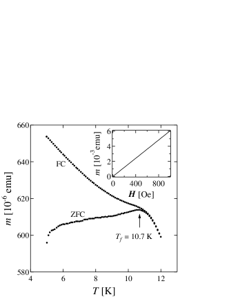
Figure 1: Temperature dependence of ZFC and FC magnetizations of Cd_0.63Mn_0.37Te in $H=100$ Oe. The freezing temperature of $\sim 10.7$K estimated by this graph. The inset shows the field dependence of the magnetization at 7K ($=T_{m}$).

The time dependence of magnetization was measured according to the following procedure. (Fig. 2) The sample was zero-field-cooled down to $T_{m}$ as rapidly as possible ($\sim 10$K/min) from 30K which is above the transition temperature $T_{g}$. Then, the temperature $T_{m}$ was held for $t_{\rm w}$ (=3000s) (initial aging stage). After that, the perturbation was given to the sample during $t_{\rm p}$ using the photo illumination (perturbation stage). After the light was turned off, a magnetic field $H$ of 100 Oe, at which the linear field-dependent magnetization was held (inset of FIG. 1)), was subsequently applied. After $t_{\rm s}\sim 60$s, the magnetic field $H$ of 100 Oe is stabilized, and then the magnetization $M$ was measured as a function of time $t$ (healing stage).

The dynamics of a spin glass below $T_{g}$ is governed by excitations of the droplet.Fisher, Huse (1988a) The size $L_{T_{m}}(t)$ of the droplet, which was thermally activated at $T_{m}$ within the time scale $t$, is given by the following equation,Fisher, Huse (1988a)

$$L_{T_{m}}(t)\sim L_{0}{\left[\frac{k_{B}T_{m}\ln(t/\tau_{0})}{\Delta(T_{m})}\right]}^{1/\psi}.$$ (1)

Consequently, a significant difference in time scales existed even between two close temperatures, $T_{m}$ and $T_{m}+\Delta T$. Therefore, we define the effective duration $t_{\rm eff}(T_{m})$ of the perturbation Yoshino et al. (2001) according to

$$L_{T_{m}+\Delta T}(t_{p})=L_{T_{m}}(t_{\rm eff}),$$ (2)

or

$$t_{\rm p}(T_{m}+\Delta T)=\tau_{0}(t_{\rm eff}(T_{m})/\tau_{0})^{T_{m}/(T_{m}+\Delta T)},$$ (3)

where $\tau_{0}$ ($\sim\hbar/J\sim 10^{-13}$s ) is a microscopic time scale.tau_value When we discuss the data below, we convert the actual duration of the perturbation $t_{\rm p}(T_{m}+\Delta T)$ into the effective duration $t_{\rm eff}(T_{m})$.

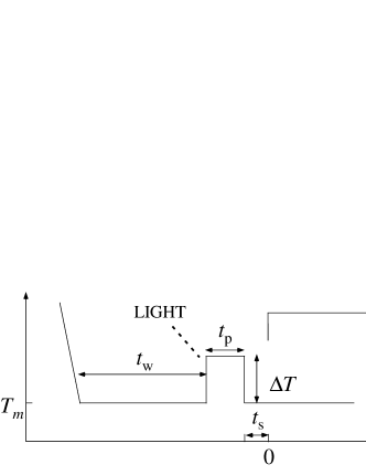
Figure 2: Experimental protocol of bond-cycling process under photo illumination. The sample was first cooled to $T_{m}=7$K and aged during $t_{\rm w}=3000$s (initial aging stage). The perturbation was subsequently added during $t_{\rm p}$ (perturbation stage) using photo illumination. After the perturbation was stopped, $H$ of 100 Oe was applied and the magnetization was measured as a function of $t$ (healing stage).

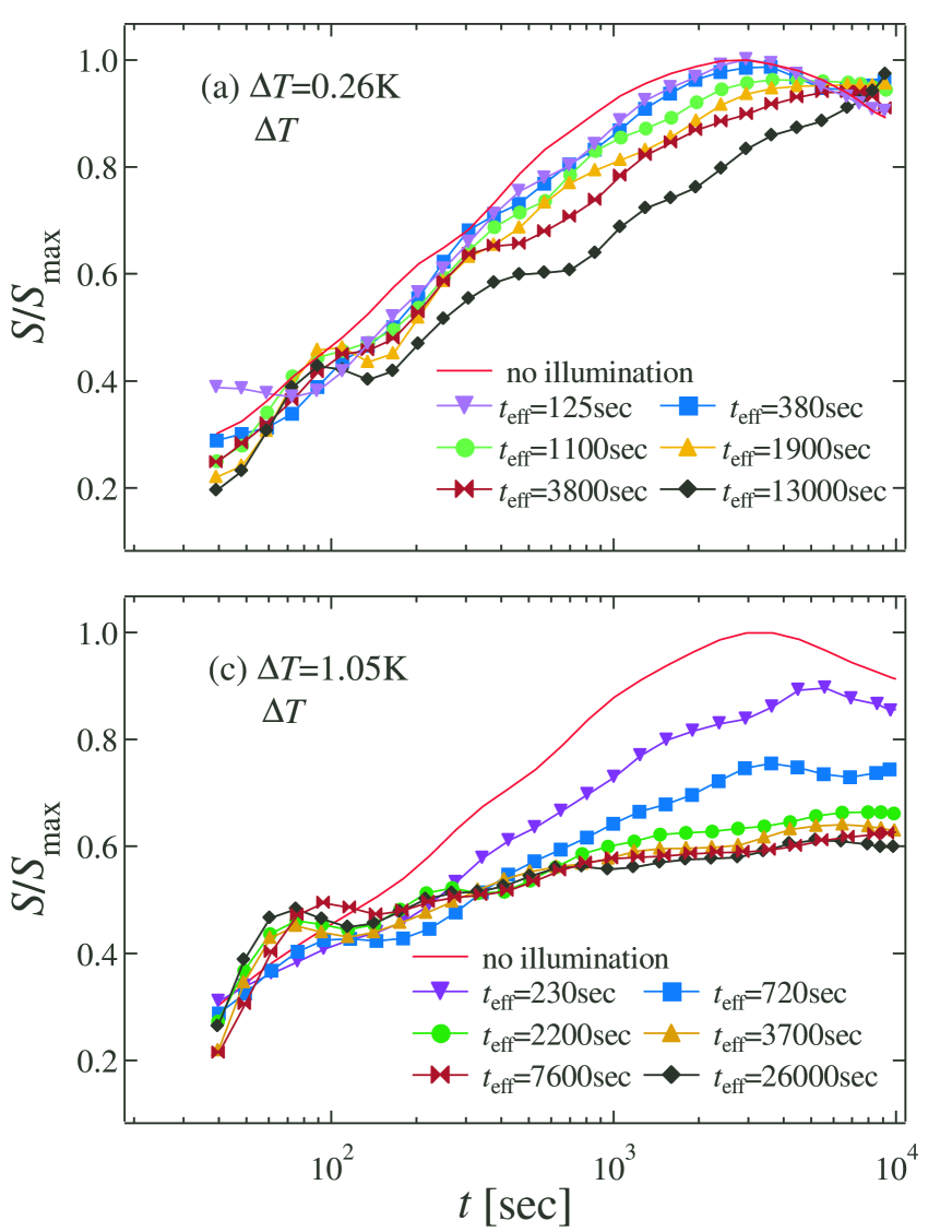
Figure 3: (Color online) Time dependence of the relaxation rate $S$ at 7K. Solid curves show $S$, measured after the waiting time $t_{\rm w}=3000$s without illumination (isothermal aging). Figure (a) (filled symbol) and (b) (open symbol) show the relaxation rates $S$ at various $t_{\rm eff}$ for $\Delta T=0.26$K under $\Delta T$ and $\Delta T+\Delta J$ perturbations, respectively. Figure (c) (filled symbol) and (d) (open symbol) show the relaxation rates $S$ at various $t_{\rm eff}$ for $\Delta T=1.05$K under $\Delta T$ and $\Delta T+\Delta J$ perturbations, respectively. All the data are normalized by the maximum height of $S$ without photo illumination.

III EXPERIMENTAL RESULTS

We focused on the relaxation rate of the magnetization, $S=(1/H)dM/d\log t$, measured under the various conditions of strength and duration of the perturbation. Since we observed the peaks in the perturbation time-dependent data of $S$, the height of each peak and the corresponding peak position are important for our discussion.

The solid curves in FIG. 3 show the time dependence of the relaxation rate $S$, measured after the aging time $t_{\rm w}=3000$s without illumination (isothermal aging). These curves show a peak at $t\sim 3000$s, which is a typical behavior observed in many spin glasses.Granberg et al. (1988)

FIG. 3 also shows the typical data of perturbation time-dependent $S$ at $T_{m}$ (=7K) of the sample, where the constant temperature increment $\Delta T$ (=0.26K, 1.05K) is added during $t_{\rm eff}$ for the perturbation. The left figures ((a) and (c)) and the right figures ((b) and (d)) show the data under $\Delta T$ and $\Delta T+\Delta J$ perturbations, respectively. All the data are normalized by the maximum height of $S$ without photo illumination. In FIGs. 3(a) and 3(b) ($\Delta T=0.26$K), the peak in $S$ at $t\sim t_{\rm w}$ (we call this the main peak) becomes gradually depressed compared with the isothermal aging curve as $t_{\rm eff}$ increases. The depression of $S$ in Fig. 3(b) is more pronounced than that in FIG. 3(a) at the same $t_{\rm eff}$. In addition, the peak position in the main peak shifts to a longer time as $t_{\rm eff}$ increases in both FIGs. 3(a) and 3(b). In FIGs. 3(c) and 3(d) ($\Delta T=1.05K$), the main peak in $S$ is depressed with increasing $t_{\rm eff}$ in a more pronounced way compared with the data at $\Delta T=0.26$K. For long $t_{\rm eff}$, $S$ becomes almost flat, but the main peak is incompletely erased. Furthermore, in FIGs. 3(c) and 3(d), a small peak appears around $t\sim 100$s (we call this the sub peak) except for short $t_{\rm eff}$, and the sub-peak becomes more pronounced with increasing $t_{\rm eff}$. The sub-peak in FIG. 3(d) is less sensitive to $t_{\rm eff}$ compared with that in FIG. 3(c). In FIG. 3(d), the sub-peak is so close to the main peak that the two peaks are insufficiently separable. We note that some curves in $S$ in FIG. 3 show a sudden increase at large values of $t$ (e.g., S for $t_{\rm eff}\sim 7600$s in FIG. 3(d) ($\Join$ symbols)). This may be due to a small fluctuation in the sample temperature.

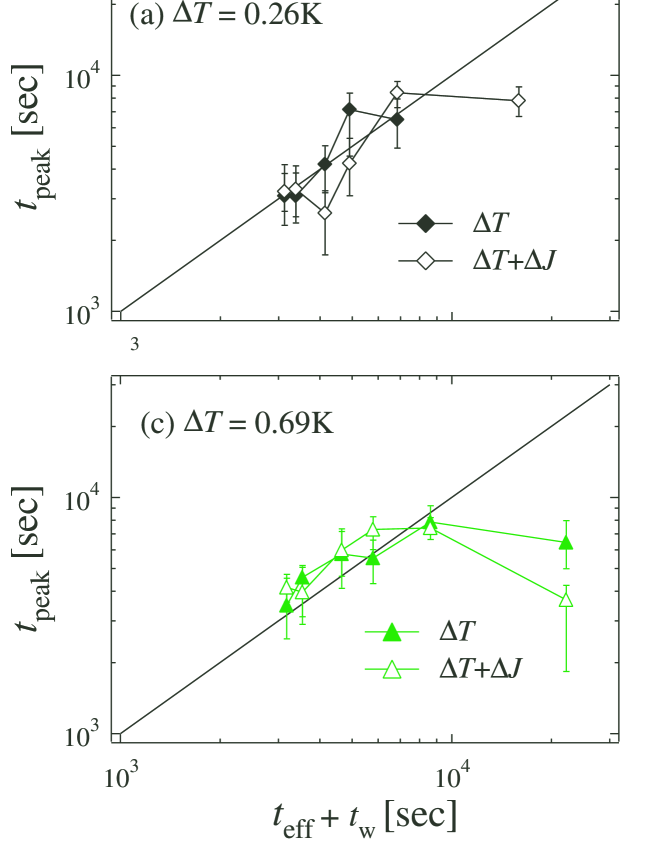
Figure 4: (Color online) The $t_{\rm eff}+t_{\rm w}$ dependent $t_{\rm peak}$ at various values of $\Delta T$. The increments of temperature under photo illumination, $\Delta T$, are 0.26K, 0.40K, 0.69K, 1.05K. Solid lines satisfies the equation $t_{\rm peak}=t_{\rm w}+t_{\rm eff}$. Filled symbols and open symbols show $t_{\rm peak}$ under $\Delta T$ and $\Delta T+\Delta J$ perturbations, respectively. The inset shows $t_{\rm eff}$-dependent $t^{\prime}_{\rm peak}$. The symbols in the inset correspond to those in the main frame.

IV DISCUSSION

IV.1 Theory based on the ghost domain scenario

Recently, aging behavior under the bond or temperature cycle has been explained based on the behavior of domains in terms of the ghost domain picture.Yoshino et al. (2001); Yoshino (2003); Jonsson, Mathieu, Nordblad, Yoshino, Aruga Katori, Ito (2004) In the following paragraphs, we interpret our results based on the behavior of the domain under the bond or temperature cycle in the same way. We divide our experimental protocol into three stages according to Fig. 2: the initial aging stage in which the equilibrium state $\Gamma_{A}$ belongs to the environment $A-(T_{m},J)$, the perturbation stage in which the equilibrium state $\Gamma_{B}$ belongs to the new environment $B-(T_{m}+\Delta T,J+\Delta J)$, and the healing stage at the environment $A$.

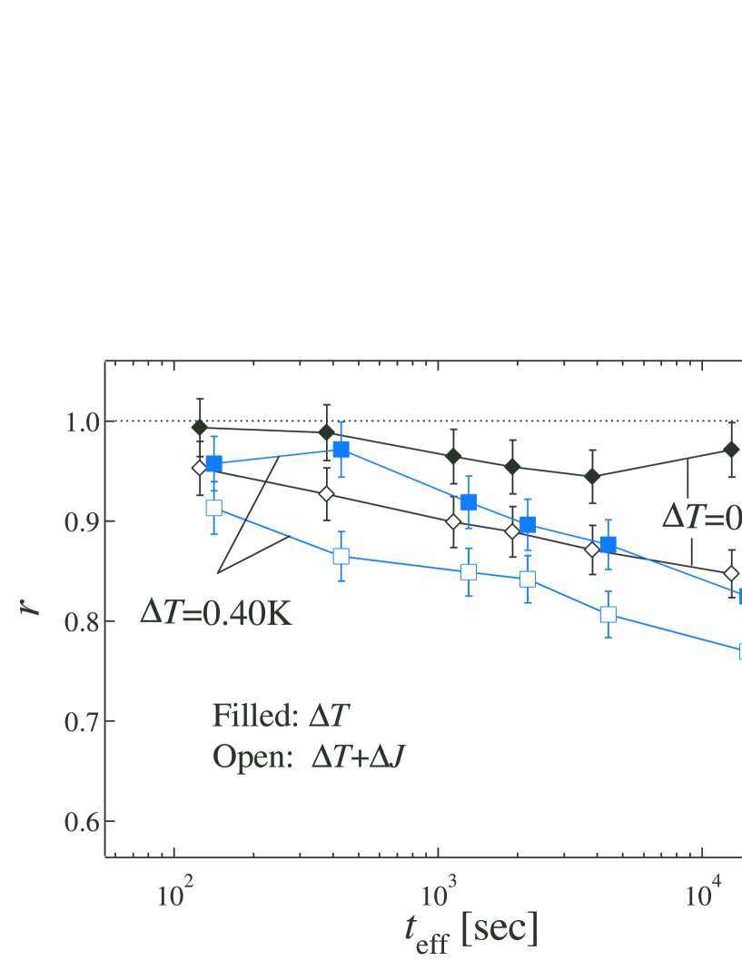
Figure 5: (Color online) The $t_{\rm eff}$ dependent $r$ at various values of $\Delta T$. The increments of temperature under photo illumination, $\Delta T$, are 0.26K, 0.40K, 0.69K and 1.05K. The filled and open symbols show $r$ under $\Delta T$ and $\Delta T+\Delta J$ perturbations, respectively. The inset shows $t_{\rm eff}$-dependent $r^{\prime}$. The symbols in the inset correspond to those in the main frame.

In the initial aging stage, the domains belonging to $\Gamma_{A}$ at $T_{m}$ grow during $t_{\rm w}$ according to Eq. (1). In the perturbation stage, the perturbation $\Delta X$ ($\Delta T$ or $\Delta T+\Delta J$) is applied from $t_{\rm w}$ to $t_{\rm w}$+$t_{\rm p}$. During the perturbation stage, the ”overlap” between the equlibrium states $\Gamma_{A}$ and $\Gamma_{B}$ disappears at the length scale beyond the overlap length $L_{\Delta X}$. The relation between $L_{\Delta X}$ and the perturbation $\Delta X$ is given as bray,Moore (1987); Fisher, Huse (1988a):

$$L_{\Delta X}=L_{0}|\Delta X/J|^{-1/\zeta}.$$ (4)

The chaos exponent $\zeta$ is given by $\zeta=d_{s}/2-\theta$ $(>0)$, where $d_{s}$ is a fractal dimension and $\theta$ is a stiffness exponent. Theoretically, temperature and bond perturbations are equivalent with respect to the overlap length $L_{\Delta X}$.Yoshino (2003)

We can distinguish the weakly and strongly perturbed regimes based on the relationship between overlap length $L_{\Delta X}$ and the domain size grown during each stages. Yoshino (2003); Jonsson, Mathieu, Nordblad, Yoshino, Aruga Katori, Ito (2004) If $L_{T_{m}+\Delta T}(t_{\rm p})<L_{\Delta X}$, a weakly perturbed regime appears, in which the rejuvenation scarcely emerges.Jonsson et al. (2003) If all the $L_{T_{m}}(t_{\rm w})$, $L_{T_{m}+\Delta T}(t_{\rm p})$, and $L_{T_{m}}(t)$ are greater than $L_{\Delta X}$, a strongly perturbed regime appears, in which the initial spin configuration is unstable with respect to droplet excitation and a new equilibrium state appears. This suggests a chaotic nature. The chaos, however, does not appear abruptlyScheffler et al. (2003); Sales et al. (2002), and there exists a crossover between the weakly and strongly perturbed regimes.

In the weakly perturbed regime, the domain belonging to $\Gamma_{A}$ is weakly modified and the order parameter $\rho$ slowly decreases in the perturbation stage. The order parameter in the domains is easily recovered during the healing stage. Thus, the recovery time $\tau_{\rm rec}$, which is necessary for the order parameter to saturate to 1, is given as

$${\tau}_{\rm rec}^{\rm weak}\sim t_{\rm eff}.$$ (5)

In this regime, the size of domain belonging to $\Gamma_{A}$ grows accumulatively so as to neglect the perturbation.

In the strongly perturbed regime, the spin configuration in domains belonging to $\Gamma_{A}$ is completely random beyond the length scale of $L_{\Delta X}$, and the domains belonging to $\Gamma_{B}$ grow during the perturbation stage. However, the effect of the initial domain of $\Gamma_{A}$ remains as a ghostYoshino (2003); Jonsson, Mathieu, Nordblad, Yoshino, Aruga Katori, Ito (2004), i.e., the domains, that grow up to $L_{T_{m}}(t_{\rm w})$ during initial aging, can vaguely keep their overall shapes (which are called ghost domain), and the domain interiors are significantly modified due to the growth of domains $\Gamma_{B}$. Thus, the order parameter $\rho$ significantly decreases (but does not reach zero). When the perturbation is removed, the system recovers the initial spin configuration (healing stage). The recovery time $\tau_{\rm rec}$ is given as

$$\tau_{\rm rec}^{\rm strong}\gg t_{\rm eff}.$$ (6)

In this regime, the domain belonging to $\Gamma_{A}$ grows non-accumulatively.

IV.2 The role of the relaxation rate under the cycling

The relaxation rate $S$ is characterized under the temperature or bond perturbations shown in Sec. IV.1, through the peak position and height in the time dependent $S$. First, we define the characteristic time $t_{\rm peak}$ corresponding to the position of the main peak. The value of $t_{\rm peak}$ is shown as a function of $t_{\rm eff}+t_{\rm w}$ in FIG. 4 D If the aging is accumulative, the spin configuration at $T_{m}+\Delta T$ in the perturbation stage is equivalent to that under the isothermal aging at $T_{m}$ for $t_{\rm eff}$. This results in the following relation:

$$t_{\rm peak}\sim t_{\rm w}+t_{\rm eff},$$ (7)

which corresponds to the reference line in FIG. 4. In the strongly perturbed regime ($L\gg L_{\Delta X}$), on the other hand, the chaotic nature becomes effective and the position of the main peak shifts to a shorter time compared with the accumulative aging curve. In this case, $t_{\rm peak}$ satisfies the relation,

$$t_{\rm peak}<t_{\rm w}+t_{\rm eff}.$$ (8)

During the healing stage, the order parameter of $\Gamma_{A}$ starts to restore the domain structure grown during initial aging, and this is probably reflected in the height of the main peak. Thus, in order to characterize the change in the peak built in $S$, we define the relative peak height $r$, which is the ratio of the height in the main peak under the perturbation to that without perturbation. In other words, $r$ is the measure of the memory after the perturbation.Jonsson, Mathieu, Nordblad, Yoshino, Aruga Katori, Ito (2004) The value of $r$ is shown as a function of $t_{\rm eff}$ in FIG. 5.

In the completely weakly perturbed regime ($L_{T_{m}}(t_{\rm eff})\ll L_{\Delta X}$), the order parameter fully recovers at $t\sim t_{\rm peak}$ according to Eq. (5). However, close to the strongly perturbed regime (the crossover regime between the weakly and strongly perturbed regimes), the order parameter does not completely recover at $t=t_{\rm w}+t_{\rm eff}$. This leads to the decrease in the height of main peak. In the strongly perturbed regime, the order parameter insufficiently recovers because of the long recovery time ${\tau}_{\rm rec}^{\rm strong}$ given in Eq. (6). Thus, $r$ is gradually depressed as $t_{\rm eff}$ increases because of the rapid increase in ${\tau}_{\rm rec}^{\rm strong}$. In addition, when the period $t_{\rm s}$ is necessary until the applied field is stabilized in a superconducting magnet after the perturbation is removed, the domain grows for $t_{\rm s}$ up to the size $L_{T_{m}}(t_{\rm s})$. This reflects the sub-peak.Jonsson, Mathieu, Nordblad, Yoshino, Aruga Katori, Ito (2004) Thus, the sub-peak becomes pronounced as the rejuvenation effects become clear.

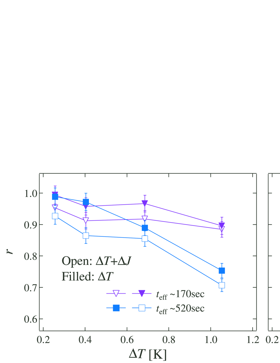
Figure 6: (Color online) The $\Delta T$-dependent $r$ at various values of $t_{\rm eff}$. Almost the same values of $t_{\rm eff}$ are gathered together in one graph. The left, middle, and right figures show $r$ under $t_{\rm eff}\sim 170$ and $520$s, $t_{\rm eff}\sim 1400$ and $2300$s, and $t_{\rm eff}\sim 4400$ and 18000s, respectively. THe filled and open symbols show $r$ under $\Delta T$ and $\Delta T+\Delta J$ perturbations, respectively.

IV.3 Bond-cycling experiment

We try to classify our data, obtained under various perturbation conditions, into the following four categories: the weakly perturbed regime (we call this the $W$ regime); the crossover regime, which is close to the weakly perturbed regime (we call this the $WC$ regime); the crossover regime, which is close to the strongly perturbed regime (we call this the $SC$ regime); and the strongly perturbed regime (we call this the $S$ regime). The criteria for the classification are abridged in TABLE 1. The classification is mainly performed based on FIG. 4 and FIG. 5 in which $t_{\rm peak}$ and $r$ are arranged as a function of $t_{\rm eff}$ under various amplitudes of $\Delta T$. The condition, i.e., $t_{\rm eff}$ is variable and $\Delta T$ is constant, corresponds to the situation that the domain size $L_{T_{m}}(t_{\rm eff})$ grown during the perturbation stage is variable while the overlap lengths $L_{\Delta T}$ and $L_{\Delta T+\Delta J}$ are constant. In addition, we also pay attention to the sub-peak whose position and relative height are shown as $t^{\prime}_{\rm peak}$ and $r^{\prime}$ in the insets in FIG. 4(d) and FIG. 5(b), respectively.

First we pay attention to the data at $\Delta T=0.26$K under $\Delta T$ perturbation. As shown in FIG. 4(a), the values of $t_{\rm peak}$ almost merge into the reference curve except for the data at the longest $t_{\rm eff}+t_{\rm w}$, where the main peak for the longest $t_{\rm eff}$ should appear at time much longer than the present observation time window ($\sim 10^{4}$s). The sub-peak cannot be observed, and $r$ scarcely decreases from 1 (FIG .5). Therefore, all the data at $\Delta T=0.26$K under $\Delta T$ perturbation satisfy the criteria for the $W$ regime in Table1. Thus, the accumulative aging proceeds in this condition.

Under the $\Delta J$ perturbation in addition to $\Delta T=0.26$K, the $t_{\rm peak}$ except for the longest $t_{\rm eff}$ satisfies Eq. (7), and the $t_{\rm peak}$, at the longest $t_{\rm eff}$, is shorter than $t_{\rm w}+t_{\rm eff}$ (FIG. 4(a)). The value of $r$ clearly decreases from 1 except for the shortest $t_{\rm eff}$ (FIG. 5). This indicates that $\Delta J$ perturbation decreases the overlap length according to Eq. (4). Under $\Delta T+\Delta J$ perturbation with $\Delta T$=0.26K, thus, the system is not completely in the $W$ regime except for the shortest $t_{\rm eff}$, and the chaotic nature partially emerges. Thus, this regime is in the $WC$ regime except for the shortest $t_{\rm eff}$, at which the system belongs to the $W$ regime.

Under both the perturbations with $\Delta T=0.40$K (see Fig 4(b)), the values of $t_{\rm peak}$ almost merge into the reference curve except for the data at the longest $t_{\rm eff}+t_{\rm w}$. At the longest $t_{\rm eff}+t_{\rm w}$, the values of $t_{\rm peak}$ under both the perturbations merge together, but lie below the reference curve. Under $\Delta T$ perturbation, $r$ is clearly lower than 1 except for the small $t_{\rm eff}$, while $r$ under $\Delta T+\Delta J$ perturbation is clearly lower than 1 over all range of $t_{\rm eff}$ (FIG. 5). The sub-peak cannot be observed under either perturbations. Therefore, at $\Delta T=0.40$K under the $\Delta T$ perturbation, the system belongs to the $WC$ regime except for short $t_{\rm eff}$, at which the system belongs to the $W$ regime. Under the $\Delta T+\Delta J$ perturbation, the system belongs to the $WC$ regime.

Next, we turn to the data under the strongest perturbation ($\Delta T=1.05$K) prior to the discussion of complex behavior under the medium perturbation ($\Delta T=0.69$K). At $\Delta T=1.05$K, $t_{\rm peak}$ cannot be determined at $\Delta T=1.05$K because the $S$ curves are so flattened except for the short $t_{\rm eff}$ (see FIG. 4(d)). The value of $r$ rapidly decreases as $t_{\rm eff}$ increases and becomes almost constant in the long $t_{\rm eff}$ region, in which $r$ under both the perturbations merge (FIG. 5). The sub-peak under $\Delta T$ perturbation is observed except for the shortest $t_{\rm eff}$ and becomes pronounced with increasing $t_{\rm eff}$ (see the inset of FIG.5). In the strongly perturbed regime, the chaotic effect significantly emerges and the main peak satisfies Eq. (8). In addition, the sub-peak, which is attributed to the rejuvenation, is observed around the time necessary to stabilize the applied field, i.e., $t_{\rm s}\sim 100$s. Under the perturbation with $\Delta T=1.05$K, thus, the system at long $t_{\rm eff}$ may be in the $S$ regime, where the order parameter $\rho$ becomes saturated to a level common to both kinds of perturbations and the rejuvenation effect becomes noticeable. Except for the long $t_{\rm eff}$, the system would not necessarily be classified into the $S$ regime, because $\rho$ is not saturated although the sub-peak is observable. Therefore, this system may belong to the $SC$ regime. The system at the shortest $t_{\rm eff}$ under $\Delta T$ perturbation is classified into the $WC$ regime because of the absence of the sub-peak.

At $\Delta T=0.69$K, $t_{\rm peak}$ almost merges into the reference curve except for the data at the longest $t_{\rm eff}+t_{\rm w}$. At the longest $t_{\rm eff}$, however, the $t_{\rm peak}$ under $\Delta T+\Delta J$ perturbation is shorter than that under $\Delta T$ perturbation. Moreover, the sub-peak appears under $\Delta T+\Delta J$ perturbation only at the longest $t_{\rm eff}$ (see the inset of FIG. 4). Under both the perturbations with $\Delta T=0.69$K, $r$ rapidly decreases from 1 as $t_{\rm eff}$ increases, but does not become saturated (FIG. 5). Under the $\Delta T+\Delta J$ perturbation with $\Delta T=0.69$K, thus, the system at the longest $t_{\rm eff}$ gets into the $SC$ regime, whereas it does not under the $\Delta T$ perturbation. Under the $\Delta T$ perturbation with $\Delta T=0.69$K, the system belongs to the $WC$ regime except for the shortest observation time, at which it belongs to the $W$ regime because $r$ scarcely deviates from 1.

To clearly evaluate the overlap length under both the perturbations, $r$ is abridged under the condition that $t_{\rm eff}$ is constant and $\Delta T$ is variable (FIG. 6). This mirrors the situation that the domain size grown during the perturbation stage is fixed while the overlap length $L_{\Delta T+(\Delta J)}$ is varied. At the shortest $t_{\rm eff}$ ($\sim 170$s) under $\Delta T$ perturbation, $r$ scarcely deviates from 1 as $\Delta T$ increases. This indicates that $\tau_{\rm rec}$ is so short that the order parameter in ghost domains easily recovers. At long $t_{\rm eff}$, $r$ rapidly decreases as $\Delta T$ increases. This shows the crossover from the weakly to the strongly perturbed regimes through the decrease in the overlap length. The values of $r$ are smaller under $\Delta T+\Delta J$ perturbation than under $\Delta T$ perturbation, but the difference in $r$ between the perturbations becomes indistinct as $\Delta T$ increases. Ultimately it disappears at large $\Delta T$ due to the extremely long recovery time.

Table 1: The defenition of classification of our data under various perturbation conditions. (1) The condition $t_{\rm peak}=t_{\rm eff}+t_{w}$ is satisfied. (2) Sub peak is observed. (3) The condition $r\sim 1$ is satisfied. (4) The value of r attains the saturation value. For example, the data that belongs to the $W$ regime satisfy the conditon (1) and (3), does not satisfy (2) and (4).

Regime	(1)	(2)	(3)	(4)
$W$	Y	N	Y	N
$WC$	Y	N	N	N
$SC$	Y	Y	N	N
$S$	N	Y	N	Y

FIG. 7 shows a schematic phase diagram in which the perturbation conditions are classified into the four regimes. In this figure, the boundary curves are guides to help the eyes grasp the qualitative aspect. As $t_{\rm eff}$ and $\Delta T$ increase, a systematic change from the $W$ to the $S$ regime is observed in the case of both the $\Delta T$ and $\Delta T+\Delta J$ perturbations. In FIG. 7, we find a feature in which the boundary curve in the $\Delta T+\Delta J$ perturbation data lies below the corresponding boundary curve in the $\Delta T$ perturbation data. This can be interpreted in terms of the decrease in the overlap length due to the additional perturbation $\Delta J$.

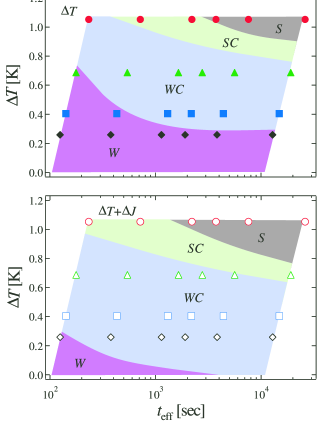
Figure 7: (Color online) Schematic phase diagram where our data are classified into the four regimes: the weakly perturbed regime ($W$ regime); the crossover regime, which is close to the weakly perturbed regime ($WC$ regime); the crossover regime, which is close to the strongly perturbed regime ($SC$ regime); the strongly perturbed regime ($S$ regime) (bottom to top). The upper and lower figures show the diagram under $\Delta T$ and $\Delta T+\Delta J$ perturbations, respectively.

IV.4 The effect of the bond perturbation

The order parameter under $\Delta T+\Delta J$ perturbation are smaller than those under $\Delta T$ perturbation with the same $\Delta T$ as mentioned above. These indicate that $\Delta J$ perturbation decreases the order parameter through the decrease in the overlap length. This is clearly demonstrated in FIG. 7 through the shift of boundary curves. The behavior of the sub-peak, observed under both perturbations with $\Delta T=1.05$K, suggests that the rejuvenation effect becomes pronounced due to the additional $\Delta J$, because the $t^{\prime}_{\rm peak}$ is longer and $r^{\prime}$ is larger under the $\Delta T+\Delta J$ perturbation than under the $\Delta T$ perturbation (see the inset of Fig. 4(d) and Fig. 5).

In addition, we pay attention to the feature in which $r$ under $\Delta T+\Delta J$ perturbation with $\Delta T=0.26$K is significantly smaller than $1$ while $r$ under $\Delta T$ perturbation is practically equal to $1$ as $t_{\rm eff}$ approaches zero, as shown in FIG. 5. This suggests that the $\Delta J$ perturbation decreases the order parameter whereas the $\Delta T$ perturbation does not, even at infinitesimal $t_{\rm eff}$. Thus, at $\Delta T=0.26$K, the effect of $\Delta T$ perturbation on the order parameter is so small that the $\Delta J$ perturbation makes the dominant contribution. Based on the feature in which $r$ under $\Delta T+\Delta J$ perturbation with $\Delta T=$0.26K is practically equal to that under $\Delta T$ perturbation at $\Delta T=0.40$K, we estimate that $\Delta J=0.14\sim 0.40$K at $\Delta T=0.26$K.

V Conclusion

The bond perturbation $\Delta J$, under photo illumination, affects the aging behavior of semiconductor spin glass. We then estimated that $\Delta J\sim 0.14\sim 0.40$K at $\Delta T=0.26$K. Thus, the bond perturbation $\Delta J$ can significantly change the bond configuration, although the photo-induced magnetization in Cd_0.63Mn_0.37Te is negligible small.Kawai,Sato (1999) This effect cannot be explained in terms of the strong separation of the time scales on different length scales. We attribute it to the decrease in the overlap length, i.e. $L_{\Delta T+\Delta J}<L_{\Delta T}$. Furthermore, we observed the crossover from weakly to strongly perturbed regimes in the bond cycling accompanied by the temperature cycling. These experimental results strongly suggest that ”chaos” and the overlap length, which are the key concepts in the droplet picture, exist because the contribution of bond perturbation appears only in the overlap length.

In the future, it will be necessary to conduct the ”pure” bond cycling experiment under photo illumination where there is no change in temperature. In addition, the mechanism of the bond perturbation using photo illumination should be clarified.

References

- Lundgren et al. (1983) L. Lundgren, P. Svedlindh, P. Nordblad, and O. Beckman, Phys. Rev. Lett. 51, 911 (1983).
- Jonasson et al. (1998) K. Jonason, E. Vincent, J. Hammann, J.-P Bouchaud, and P. Nordblad, Phys. Rev. Lett. 81, 3243 (1998).
- Jonsson et al. (1999) T. Jonsson, K. Jonason, P. Jönsson, and P. Nordblad, Phys. Rev. B. 59, 8770 (1999).
- Fisher, Huse (1988a) D. S. Fisher and D. A. Huse, Phys. Rev. B 38, 386 (1988).
- Fisher, Huse (1988b) D. S. Fisher and D. A. Huse, Phys. Rev. B 38, 373 (1988).
- bray,Moore (1987) A. J. Bray and M. A. Moore, Phys. Rev. Lett. 58, 57 (1987).
- Scheffler et al. (2003) F. Scheffler, H. Yoshino, and P. Maass, Phys. Rev. B 68, 060404(R) (2003).
- Sales et al. (2002) M. Sales, and H. Yoshino, Phys. Rev. E 65, 066131 (2002).
- Jonsson et al. (2003) P. E. Jönsson, H. Yoshino, and P. Nordblad, Phys. Rev. Lett. 90, 059702 (2003).
- Yoshino et al. (2001) H. Yoshino, A. Lemaître, and J.-P. Bouchaud, Eur. Phys. J. B 20, 367 (2001).
- Yoshino (2003) H. Yoshino, J. Phys. A 36, 10819 (2003).
- Jonsson, Mathieu, Nordblad, Yoshino, Aruga Katori, Ito (2004) P. E. Jönsson, R. Mathieu, P. Nordblad, H. Yoshino, H. Aruga Katori, and A. Ito, Phys. Rev. B 70, 174402 (2004).
- nordblad et al. (1987) P. Nordblad, P. Svedlindh, L. Sandlund, and L. Lundgren, Phys. Lett. A 120, 475 (1987).
- Granberg et al. (1988) L. Sandlund, P. Svedlindh, P. Granberg, P. Nordblad, and L. Lundgren, J. Appl. Phys. 64, 5616 (1988).
- granberg et al. (1990) P. Granberg, L. Lundgren, and P. Nordblad, J. Magn. Magn. Mater. 92, 228 (1990).
- Bert et al. (2004) F. Bert, V. Dupuis, E. Vincent, J. Hammann, and J.-P. Bouchaud, Phys. Rev. Lett. 92, 167203 (2004).
- Picco et al. (2001) M. Picco, F. Ricci-Tersenghi, and F. Ritort, Phys. Rev. B 63, 174412 (2001).
- Berthier et al. (2002) L. Berthier and J.-P. Bouchaud, Phys. Rev. B 66, 054404 (2002).
- Berthier et al. (2005) L. Berthier and A. P. Young, Phys. Rev. B 71, 214429 (2005).
- (20) J.-P. Bouchaud, V. Dupuis, J. Hammann, and E. Vincent, Phys. Rev. B 65, 024439 (2002).
- berthier et al. (2003) L. Berthier and J.-P. Bouchaud, Phys. Rev. Lett 90, 059701 (2003).
- Galazka et al. (1980) R. R. Galazka, S. Nagata, and P. H. Keesom, Phys. Rev. B 22, 3344 (1980).
- nordblad et al. (1986) P. Nordblad, P. Svedlindh, J. Ferré, and M. Ayadi, J. Magn. Magn. Mater. 59, 250 (1986).
- (24) A. Mauger, J. Ferré, M. Ayadi, and P. Nordblad, Phys. Rev. B 37, 9022 (1988); A. Mauger, J. Ferré, and P. Beauvillain, ibid. 40, R862 (1989).
- Zhou et al. (1989) Y. Zhou, C. Rigaux, A. Mycielski,M. Menant, and N. Bontemps, Phys. Rev. B 40, R8111 (1989).
- nordblad et al. (1994) M. Smith, A. Dissanayake, and H. X. Jiang, Phys. Rev. B. 49, 4514 (1994).
- sato,hori (2004) T. Sato and A. Hori, J. Magn. Magn.Mater. 272-276, 1337 (2004).
- Kawai,Sato (1999) H. Kawai and T. Sato, J. Appl. Phys. 85, 7310 (1999).
- (29) As shown in Fig.1, the FC susceptibility increases as temperature decreases, which is different from the conventional spin glass behavior. This is attributed to the paramagnetic contribution from the small magnetic clusters, which are not belonging to the freezing spins. See Ref.22.
- (30) The typical spin-flip time in spin glass has been evaluated s, e.g., s for Cd0.6Mn0.4Te and s for Cd0.55Mn0.45Te are evaluated [See A. Mauger et al., Phys. Rev. B 37, 9022(1988) and M. Saint-Paul and J. L. Tholence and W. Giriat, Solid State Commun. 60, 621(1986)]. The duration of the perturbation is insensitive to the value of , and we assume the typical spin-flip time of s in the present work.
- Granberg et al. (1988) P. Granberg, L. Sandlund, P. Nordblad, P. Svedlindh, and L. Lundgren, Phys. Rev. B 38, 7097 (1988).