Generalised extreme value statistics and sum of correlated variables

Abstract

We show that generalised extreme value statistics –the statistics of the $k^{\mathrm{th}}$ largest value among a large set of random variables– can be mapped onto a problem of random sums. This allows us to identify classes of non-identical and (generally) correlated random variables with a sum distributed according to one of the three ($k$-dependent) asymptotic distributions of extreme value statistics, namely the Gumbel, Fréchet and Weibull distributions. These classes, as well as the limit distributions, are naturally extended to real values of $k$, thus providing a clear interpretation to the onset of Gumbel distributions with non-integer index $k$ in the statistics of global observables. This is one of the very few known generalisations of the central limit theorem to non-independent random variables. Finally, in the context of a simple physical model, we relate the index $k$ to the ratio of the correlation length to the system size, which remains finite in strongly correlated systems.

1 Introduction

One of the cornerstones of probability theory is the celebrated central limit theorem, stating that under general assumptions, the distribution of the sum of independent random variables converges, once suitably rescaled, to a Gaussian distribution. This theorem provides one of the foundations of statistical thermodynamics and, from a more practical point of view, legitimates the use of Gaussian distributions to describe fluctuations appearing in experimental or numerical data.
However, this general theorem breaks down in several situations of physical interest, when the assumptions made to derive it are no longer fulfilled. For instance, if the random variables contributing to the sum have an infinite variance, the distribution of the sum is no longer Gaussian, but becomes a Lévy distribution [1]. This has deep physical consequences, for instance in the context of laser cooling [2] or in that of glasses [3, 4]. Though the central limit theorem applies to a class of correlated variables, the martingale differences [5, 6], it is generally inapplicable to sums of strongly correlated, or alternatively, strongly non-identical random variables. In this case, no general mathematical theory is available, but experimental as well as numerical distributions of the fluctuations of global observables in correlated systems often present an asymmetric shape, with an exponential tail on one side and a rapid fall-off on the other side. Such distributions are usually well described by the so-called generalised Gumbel distribution with a real index $a$. The latter is one of the limit distributions appearing, for integer values $a=k$, as the distribution of the $k^{\mathrm{th}}$ extremal value of a set of independent and identically distributed random variables [7, 8]. For instance, Bramwell and co-workers argued that the generalised Gumbel distribution with $a\approx 1.5$ reasonably describes the large scale fluctuations in many correlated systems [9]. Since then, the generalised Gumbel distribution has been reported in various contexts [10, 11, 12, 13, 14]. Yet, the interpretation of such a distribution in the context of extreme value statistics (EVS) is far from obvious. This issue led to a debate around the possible existence of a (hidden) extreme process which might dominate the statistics of sums of correlated variables in physically relevant situations [15, 16, 17, 18]. Still, no evidence for such a process has been found yet. And even if one accepts that some extremal process is at play, a conceptual difficulty remains, as speaking of the $k^{\mathrm{th}}$ largest value for non-integer $k$ simply does not make sense.
In this article we propose another interpretation of the usual EVS in terms of statistics of sums of correlated variables. Within this framework the extension to real positive values of $k$ is straightforward and avoids any logical problem. Usual EVS then appears as a particular case of a more general problem of limit theorem for sums of correlated variables belonging to a given class.
The article is organised as follows. In Section 2 we present the link between usual EVS and sums of correlated variables, and propose a more general problem of random sums, which is studied is the next sections. In Section 3, we present in detail the simple problem of sum –already presented shortly by one of us in a previous publication [19]– associated with the EVS of exponential random variables. Section 4 deals with the extension to the more general problem of random sums defined in Section 2, and it is shown that the asymptotic distribution of the sum, is either a (generalised) Gumbel, Fréchet or Weibull distribution. Finally, we discuss in Section 5 some physical interpretations of our results.

2 Equivalence between extreme value statistics and sums of correlated variables

2.1 Standard extreme value statistics

The asymptotic theory of EVS, which found applications for instance in physics [20], hydrology [21], seismology [22] and finance [23], is also part of the important results of probability theory. Consider a random variable $X$, distributed according to the probability density $P$, and let $\mathfrak{X}_{N}$ be a set of $N$ realisations of this random variable. Now instead of considering the sum of these $N$ realisations as in the central limit theorem, one is interested in the study of the distribution of the $k^{\mathrm{th}}$ maximal value $z_{k}$ of $\mathfrak{X}_{N}$. The major result of EVS is that, in the limit $N\rightarrow\infty$, the probability density of $z_{k}$ does not depend on the details of the original distribution $P$: There are only three different types of distributions, depending on the asymptotic behaviour of $P$ [7, 8]. In particular, in the case where $P$ decreases faster than any power laws at large $x$, the variable $z_{k}$ is distributed according to the Gumbel distribution

$$G_{k}(z_{k})=\frac{k^{k}\theta_{k}}{\Gamma(k)}\exp\left[-k\theta_{k}(z_{k}+\nu_{k})-ke^{-\theta_{k}(z_{k}+\nu_{k})}\right],$$ (1)

$$\theta_{k}^{2}=\Psi^{\prime}(k),\quad\nu_{k}=\frac{1}{\theta_{k}}\big{[}\ln k-\Psi(k)\big{]},$$

where $\Psi(x)=\frac{\mathrm{d}}{\mathrm{d}x}\ln\Gamma(x)$ is the digamma function. Note that from the point of view of EVS, $k\in\mathbb{N}^{*}$ by construction. Yet, if one forgets about EVS, the expression (1) is also formally valid for $k=a$ real and positive.

2.2 Reformulation as a problem of sum

Let us consider again the set $\mathfrak{X}_{N}$ defined here above. We then introduce the ordered set of random variables, $z_{k}=x_{\sigma(k)}$, where $\sigma$ is the ordering permutation such that $z_{1}\geq z_{2}...\geq z_{N}$. One can now define the increments of $z$ with the following relations:

$$u_{k} \equiv z_{k}-z_{k+1},\ \forall\ 1\leq k\leq N-1,$$

$$u_{N} \equiv z_{N}.$$

Then by definition, the following identity holds

$$z_{n}\equiv\mathop{\mathrm{Max}^{(n)}}\Big{[}\mathfrak{X}_{N}\Big{]}=\sum_{k=n}^{N}u_{k},$$ (2)

where $\mathop{\mathrm{Max}^{(n)}}$ is the $n^{\mathrm{th}}$ largest value of the set $\mathfrak{X}_{N}$, showing that an extreme value problem may be reformulated as a problem of sum of random variables $U_{k}$.
Besides, as these new random variables have been obtained through an ordering process, they are a priori non-independent and non-identically distributed. This is confirmed by the computation of the joint probability $\tilde{J}_{k,N}(u_{k},...,u_{N})$ which is given by

$$\tilde{J}_{k,N}(u_{k},...,u_{N}) = N!\int_{0}^{\infty}\mathrm{d}z_{N}P(z_{N})\int_{z_{N}}^{\infty}\mathrm{d}z_{N-1}P(z_{N-1})...\int_{z_{2}}^{\infty}\mathrm{d}z_{1}P(z_{1})$$

$$\qquad\qquad\times\delta(u_{N}-z_{N})\prod_{n=k}^{N-1}\delta(u_{n}-z_{n}+z_{n+1}),$$

$$= N!\left[\prod_{n=k}^{N}P\left(\sum_{i=n}^{N}u_{i}\right)\right]\int_{u_{k}+...+u_{N}}^{\infty}\mathrm{d}z_{k-1}P(z_{k-1})...\int_{z_{2}}^{\infty}\mathrm{d}z_{1}P(z_{1}).$$

By recurrence it is easy to demonstrate the following relation,

$$\int_{u}^{\infty}\mathrm{d}z_{k-1}P(z_{k-1})...\int_{z_{2}}^{\infty}\mathrm{d}z_{1}P(z_{1})=\frac{1}{(k-1)!}F(u)^{k-1},$$

with $F(u)\equiv\int_{u}^{\infty}\mathrm{d}z\ P(z)$, leading to

$$\tilde{J}_{k,N}(u_{k},...,u_{N})=\frac{N!}{(k-1)!}\;F\left(\sum_{i=k}^{N}u_{i}\right)^{k-1}\prod_{n=k}^{N}P\left(\sum_{i=n}^{N}u_{i}\right).$$

The probability $\tilde{J}_{k,N}$ is actually a probability at $N^{\prime}=N+1-k$ points, and a shift of indices allows one to write it in the final form:

$$\qquad\qquad J_{N^{\prime}}(u_{1},...,u_{N^{\prime}})=\frac{(N^{\prime}+k-1)!}{(k-1)!}\;F\left(\sum_{i=1}^{N^{\prime}}u_{i}\right)^{k-1}\prod_{n=1}^{N^{\prime}}P\left(\sum_{i=n}^{N^{\prime}}u_{i}\right).$$ (3)

In the general case, this expression does not factorise, i.e. one cannot find $N^{\prime}$ functions $\pi_{n}$ such that

$$J_{N^{\prime}}(u_{1},...,u_{N^{\prime}})=\prod_{n=1}^{N^{\prime}}\pi_{n}(u_{n}),$$

and the random variables $U_{n}$ are thus non-independent.

2.3 Extension of the joint probability

Up to now, we only reformulated the usual extreme value statistics as a problem of sum, by some trivial manipulations. Basically, we have two equivalent problems with the same asymptotic distribution, e.g., the standard Gumbel distribution if $P$ is in the Gumbel class. Let us now point out that Eq. (3) is a particular case of the following joint distribution

$$J_{N}(u_{1},...,u_{N})=\frac{\Gamma(N)}{Z_{N}}\;\Omega\left[F\left(\sum_{n=1}^{N}u_{n}\right)\right]\prod_{n=1}^{N}P\left(\sum_{i=n}^{N}u_{i}\right)$$ (4)

where $\Omega(F)$ is an (arbitrary) positive function of $F$, and where $Z_{N}$ is given by

$$Z_{N}=\int_{0}^{1}\mathrm{d}v\,\Omega(v)\,(1-v)^{N-1}.$$ (5)

Eq. (3) is recovered by choosing $\Omega(F)=F^{k-1}$. Note that by extending the definition of the joint probability, we lost the equivalence between the two original problems. In other words, we are generalising the problem of statistics of sums and not the extreme value one. In the rest of this article, we study the limit distribution of a sum of correlated random variables satisfying the generalised joint probability (4).
Let us note finally that one can easily generate from the joint probability (4) other joint probabilities that lead to the same asymptotic distribution for the sum, by summing over a set $\mathcal{S}$ of permutations over $[1,...,N]$

$$J_{N}^{\mathcal{S}}(u_{1},...,u_{N})=\frac{1}{\mathcal{N}(\mathcal{S})}\sum_{\sigma\in\mathcal{S}}J_{N}(u_{\sigma(1)},...,u_{\sigma(N)}),$$

$\mathcal{N}(\mathcal{S})$ being the cardinal of S. This may allow in particular some symmetry properties between the variables to be restored. Indeed, starting for instance from independent and non-identically distributed random variables, this procedure leads to a set of non-independent and identically distributed random variables with the same statistics for the sum.

3 The exponential case

Though in general the joint probability does not factorise, there is a particular case where it does. For pedagogical purposes, we discuss this case separately, before dealing with the general case in Section 4. To allow the joint probability $J_{N}$ defined by (4) to factorise, the function $P$ has to satisfy the following property:

$$\forall(x,y),\ P(x+y)=P(x)P(y).$$

That is to say that $P$ must be exponential: $P(x)=\kappa e^{-\kappa x}$, with $\kappa>0$. As a result, one has $F(x)=e^{-\kappa x}$, and the factorisation criterion on $J_{N}$ translates into the following condition on $\Omega$

$$\forall(F_{1},F_{2}),\ \Omega(F_{1}F_{2})=\Omega(F_{1})\Omega(F_{2}),$$

so that $\Omega$ must be a power law: $\Omega(F)=F^{a-1}$ (the prefactor may be set to $1$ without loss of generality), with $a>0$ to ensure the convergence of the integral defining $Z_{N}$ given in Eq. (5). In such a case, one finds

$$Z_{N}=\frac{\Gamma(N)\Gamma(a)}{\Gamma(N+a)},$$ (6)

and the joint probability could be written in the factorised form (2.2), with

$$\pi_{n}(u_{n})=(n+a-1)\kappa\,e^{-(n+a-1)\kappa u_{n}}.$$ (7)

Therefore, for $a=k$ integer, if one sums independent and non-identically distributed random variables $U_{n}$, $n=1,...,N$, obeying (7), the distribution of the sum converges to a Gumbel distribution $G_{k}$ in the limit $N\rightarrow\infty$. Note that the particular case $k=1$ has been previously studied by Antal et alin the context of $1/f$ noise [24]. In the following of this section, we shall establish that for $a$ real, the distribution of the sum of the $U_{n}$’s converges towards the generalised Gumbel distribution $G_{a}$ for $N\rightarrow\infty$, as announced in a previous publication [19].
To this aim, let us define the random sum $S_{N}=\sum_{n=1}^{N}U_{n}$, where $U_{n}$ is distributed according to (7), with $a$ real and positive. The distribution of $S_{N}$ is denoted by $\Upsilon_{N}$. As the $U_{n}$’s are independent, the Fourier transform of $\Upsilon_{N}$ is simply given by

$$\mathcal{F}\left[\Upsilon_{N}\right](\omega)=\prod_{n=1}^{N}\mathcal{F}\left[\pi_{n}\right](\omega)=\prod_{n=1}^{N}\left(1+\frac{i\omega}{\kappa(n+a-1)}\right)^{-1}.$$ (8)

The first two moments of the distribution read

$$\langle S_{N}\rangle = \sum_{n=1}^{N}\langle U_{n}\rangle=\frac{1}{\kappa}\sum_{n=1}^{N}\frac{1}{n+a-1},$$ (9)

$$\sigma_{N}^{2} = \sum_{n=1}^{N}\mathrm{Var}(U_{n})=\frac{1}{\kappa^{2}}\sum_{n=1}^{N}\frac{1}{(n+a-1)^{2}}.$$ (10)

In order to get a well-defined distribution in the limit $N\rightarrow\infty$, let us introduce the reduced variable $\mu$ by

$$\mu=\frac{s-\langle S_{N}\rangle}{\sigma},\ \mathrm{with}\ \sigma=\lim_{N\rightarrow\infty}\sigma_{N}.$$

Note that the fact that $\sigma<\infty$ breaks the Lindeberg’s condition, allowing an eventual breakdown of the central limit theorem [25]. The distribution of $\mu$, $\Phi_{N}$, is then given by $\Phi_{N}(\mu)=\sigma\Upsilon_{N}(\sigma\mu+\langle S_{N}\rangle)$. The Fourier transform of $\Phi=\lim_{N\rightarrow\infty}\Phi_{N}$ reads, using (8,9)

$$\mathcal{F}\left[\Phi_{\infty}\right](\omega)=\lim_{N\rightarrow\infty}\mathcal{F}\left[\Phi_{N}\right](\omega)=\prod_{n=1}^{\infty}\left(1+\frac{i\omega}{\sigma\kappa(n+a-1)}\right)^{-1}\exp\left(\frac{i\omega}{\sigma\kappa(n+a-1)}\right).$$

The last part of the previous expression has to be compared with the Fourier transform given in Appendix A, leading to

$$\Phi_{\infty}(\mu)=G_{a}(\mu).$$

This result shows that it is possible to obtain quite directly the generalised Gumbel distribution with a real index $a$, not from an extremal process, but from a sum of independent non-identically distributed random variables. As already pointed out, the fact that the random variables $U_{n}$ are uncorrelated is a specificity of the exponential distribution. A natural question is then to know whether this result survives for a more general class of distributions $P$ and functions $\Omega$. We address this question in the next section.

4 Generalised extreme value distributions

In the general case, the random variables $U_{n}$ are non-independent, so we have to deal with the joint probability (4). Accordingly, the route to the asymptotic limit distribution will be quite different from the exponential case.

4.1 Distribution of the sum for finite $N$

Consider a set of realisations $\{u_{n}\}$ of $N$ (correlated) random variables $U_{n}$, with the joint probability (4). We then define as above the random variable $S_{N}=\sum_{n=1}^{N}U_{n}$, and let $\Upsilon_{N}$ be the probability density of $S_{N}$. Then $\Upsilon_{N}$ is given by

$$\Upsilon_{N}(s)=\int_{0}^{\infty}\mathrm{d}u_{N}...\mathrm{d}u_{1}J_{N}(u_{1},...,u_{N})\;\delta\left(s-\sum_{n=1}^{N}u_{n}\right).$$

Inserting (4), one obtains

$$\Upsilon_{N}(s)=\frac{\Gamma(N)}{Z_{N}}\,P(s)\,\Omega\big{(}F(s)\big{)}\,I_{N}(s),$$

with

$$I_{N}(s)=\int_{0}^{\infty}\mathrm{d}u_{N}P(u_{N})\int_{0}^{\infty}\mathrm{d}u_{N-1}P(u_{N}+u_{N-1})...\int_{0}^{\infty}\mathrm{d}u_{1}\delta\left(s-\sum_{n=1}^{N}u_{n}\right).$$

To evaluate $I_{N}$, let us start by integrating over $u_{1}$, using

$$\int_{0}^{\infty}\mathrm{d}u_{1}\delta\left(s-\sum_{n=1}^{N}u_{n}\right)=\Theta\left(s-\sum_{n=2}^{N}u_{n}\right),$$

where $\Theta$ is the Heaviside distribution. This changes the upper bound of the integral over $u_{2}$ by $u_{2}^{\mathrm{max}}=\max\left(0,s-\sum_{n=2}^{N}u_{n}\right)$. Then the integration over $u_{2}$ leads to

$$\int_{0}^{u_{2}^{\mathrm{max}}}\mathrm{d}u_{2}P(u_{2})=\left[F\left(\sum_{n=3}^{N}u_{n}\right)-F(s)\right]\Theta\left(s-\sum_{n=3}^{N}u_{n}\right),$$

By recurrence it is then possible to show that

$$I_{N}(s)=\frac{1}{\Gamma(N)}\Big{(}1-F(s)\Big{)}^{N-1},$$

finally yielding the following expression for $\Upsilon_{N}$:

$$\Upsilon_{N}(s)=\frac{1}{Z_{N}}\,P(s)\,\Omega\big{(}F(s)\big{)}\,\Big{(}1-F(s)\Big{)}^{N-1}.$$ (11)

In the following sections, we assume that $\Omega(F)$ behaves asymptotically as a power law $\Omega(F)\sim\Omega_{0}\,F^{a-1}$ when $F\to 0$ ($a>0$). Under this assumption, we deduce from Eq. (11) the different limit distributions associated with the different classes of asymptotic behaviours of $P$ at large $x$.

4.2 The Gumbel class

In this section we focus on the case where $P$ is in the Gumbel class, that is, $P(x)$ decays faster than any power law at large $x$. Note that the exponential case studied above precisely belongs to this class. Our aim is to show that, after a suitable rescaling of the variable, the limit distribution obtained from (11) is the generalised Gumbel distribution $G_{a}$, where $a$ characterises the asymptotic behaviour of $\Omega(F)$ for $F\rightarrow 0$.

To that purpose, we define $s^{*}_{N}$ by $F(s^{*}_{N})=a/N$. If $a$ is an integer, this is nothing but the typical value of the $a^{\mathrm{th}}$ largest value of $s$ in a sample of size $N$. As $P$ is unbounded we have

$$\lim_{N\rightarrow\infty}s^{*}_{N}=+\infty.$$

Let us introduce $g(s)=-\ln F(s)$ and, assuming $g^{\prime}(s_{N})\neq 0$, define the rescaled variable $v$ by

$$s=s^{*}_{N}+\frac{v}{g^{\prime}(s^{*}_{N})}.$$ (12)

For large $N$, one can perform a series expansion of $g$ around $s^{*}_{N}$:

$$g(s)=g(s^{*}_{N})+v+\sum_{n=1}^{\infty}\frac{1}{n!}\frac{g^{(n)}(s^{*}_{N})}{g^{\prime}(s^{*}_{N})^{n}}\,v^{n}.$$

For $P$ in the Gumbel class, $g^{(n)}(s^{*}_{N})/g^{\prime}(s^{*}_{N})^{n}$ is bounded as a function of $n$ so that the series converges. In addition, one has

$$\lim_{N\rightarrow\infty}\frac{g^{(n)}(s^{*}_{N})}{g^{\prime}(s^{*}_{N})^{n}}=0,\ \forall n\geq 2,$$

so that $g(s)$ may be written as

$$g(s)=g(s^{*}_{N})+v+\varepsilon_{N}(v),\quad\mathrm{with}\lim_{N\rightarrow\infty}\varepsilon_{N}(v)=0.$$ (13)

Given that $P(s)=g^{\prime}(s)\,F(s)$, one gets using Eqs. (11) and (13)

$$\Phi_{N}(v) = \frac{1}{g^{\prime}(s_{N}^{*})}\Upsilon_{N}(s)$$

$$= \frac{1}{Z_{N}}\frac{g^{\prime}(s)}{g^{\prime}(s_{N}^{*})}\,F(s)\,\Omega\big{(}F(s)\big{)}\Big{(}1-F(s)\Big{)}^{N-1},$$

where $s$ is given by Eq. (12). For $P$ in the Gumbel class, it can be checked that, for fixed $v$

$$\lim_{N\rightarrow\infty}\frac{g^{\prime}\big{(}s_{N}^{*}+v/g^{\prime}(s_{N}^{*})\big{)}}{g^{\prime}(s_{N}^{*})}=1.$$

Besides, $F\big{(}s_{N}^{*}+v/g^{\prime}(s_{N}^{*})\big{)}\rightarrow 0$ when $N\rightarrow\infty$, so that one can use the small $F$ expansion of $\Omega(F)$. Altogether, one finds

$$\Phi_{N}(v)\sim\frac{\Omega_{0}}{Z_{N}}\left(\frac{a}{N}\right)^{a}e^{-av-a\varepsilon_{N}(v)}\left[1-\frac{a}{N}\,e^{-v-\varepsilon_{N}(v)}\right]^{N-1}$$

Using a simple change of variable in Eq. (5), one can show that

$$\lim_{N\rightarrow\infty}\frac{N^{a}Z_{N}}{\Omega_{0}}=\Gamma(a)$$

It is then straightforward to take the asymptotic limit $N\to\infty$, leading to

$$\Phi_{\infty}(v)=\frac{a^{a}}{\Gamma(a)}\exp\left[-av-ae^{-v}\right].$$

In order to recover the usual expression for the generalised Gumbel distribution, one simply needs to introduce the reduced variable

$$\mu=\frac{v-\langle v\rangle}{\sigma_{v}},$$

with, $\Psi$ being the digamma function,

$$\langle v\rangle=\ln a-\Psi(a),\quad\sigma_{v}^{2}=\Psi^{\prime}(a).$$

The variable $\mu$ is then distributed according to a generalised Gumbel distribution (1).
To sum up, if one considers the sum $S_{N}$ of $N\gg 1$ random variables linked by the joint probability (4), then the asymptotic distribution of the reduced variable $\mu$ defined by

$$\mu=\frac{s_{N}-\langle S_{N}\rangle}{\sigma_{N}},$$

with

$$\langle S_{N}\rangle=s^{*}_{N}+\frac{\ln a-\Psi(a)}{g^{{}^{\prime}}(s^{*}_{N})},\quad\sigma_{N}=\frac{\sqrt{\Psi^{\prime}(a)}}{g^{{}^{\prime}}(s^{*}_{N})}.$$

is the generalised Gumbel distribution (1). More generally, the approach developed in this paper to relate EVS with sums of non-independent random variables, and then generalise the problem of sum, may be summarised as shown on Fig. 1 on the example of the Gumbel class.

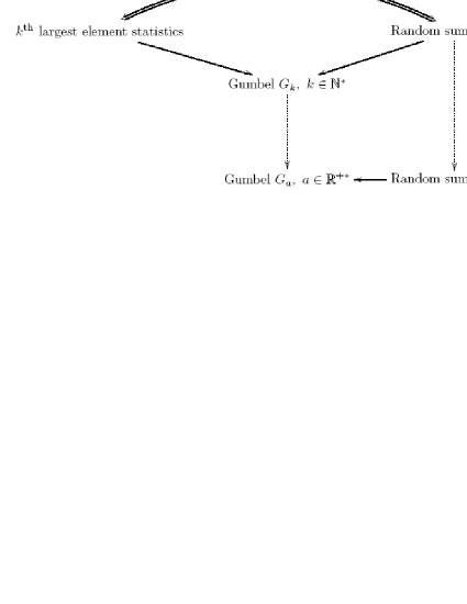
Figure 1: Generalisation of EVS via sums of non-independent variables.

4.3 Extension to the Fréchet and Weibull classes

Let us now consider the cases where $P$ belongs either to the Fréchet class, that is $P$ has a power law tail

$$P(x)\mathop{\hbox to0.0pt{\hss${}\sim{}$}}\limits_{\;\;x\rightarrow\infty}\frac{P_{0}}{x^{1+\eta}},\quad\eta>0,$$

with $P_{0}>0$ a constant, or to the Weibull class, that is $P$ has an upper bound $A$ and behaves as a power law in the vicinity of $A$

$$\forall x>A,\ P(x)=0$$

$$P(x)\mathop{\hbox to0.0pt{\hss${}\sim{}$}}\limits_{\;\;x\rightarrow A^{-}}\tilde{P}_{0}\,(A-x)^{\beta-1},\quad\beta>0.$$ (14)

with $\tilde{P}_{0}$ an arbitrary positive prefactor. A calculation similar to the one used in the Gumbel case allows the asymptotic distributions to be determined. Considering first the Fréchet class, we define $s_{N}^{*}$ through $F(s_{N}^{*})=a/N$ as above, and introduce the scaling variable $v=s/s_{N}^{*}$. This gives for the distribution $\Phi_{N}^{\mathrm{f}}(v)$

$$\Phi_{N}^{\mathrm{f}}(v)\sim\frac{a^{a}\Omega_{0}}{N^{a}Z_{N}}\frac{\eta}{v^{1+a\eta}}\left(1-\frac{a}{Nv^{\eta}}\right)^{N-1}.$$

Taking the limit $N\rightarrow\infty$, the asymptotic distribution reads

$$\Phi_{\infty}^{\mathrm{f}}(v)=\frac{a^{a}}{\Gamma(a)}\frac{\eta}{v^{1+a\eta}}e^{-a/v^{\eta}}.$$

One can rescale the variable $v$ with respect either to the mean value or to the standard deviation $\sigma$. In this latter case, one finds

$$\sigma=\frac{a^{1/\eta}}{\Gamma(a)}\left[\Gamma(a)\Gamma\left(a-\frac{2}{\eta}\right)-\Gamma\left(a-\frac{1}{\eta}\right)^{2}\right]^{1/2}.$$

Introducing $\mu=v/\sigma$ we get

$$F_{a}(\mu) = \frac{\eta\Lambda^{a}}{\Gamma(a)}\frac{1}{\mu^{1+a\eta}}\exp\left(-\Lambda\mu^{-\eta}\right),$$

$$\Lambda = \Gamma(a)^{\eta}\left[\Gamma(a)\Gamma\left(a-\frac{2}{\eta}\right)-\Gamma\left(a-\frac{1}{\eta}\right)^{2}\right]^{-\eta/2}.$$

Calculations for the Weibull class are very similar, given that the scaling variable is now $v=(A-s)/(A-s_{N}^{*})$. Skipping the details, the asymptotic distribution reads

$$\Phi_{\infty}^{\mathrm{w}}(v)=\frac{\beta\,a^{a}}{\Gamma(a)}\,v^{a\beta-1}e^{-av^{\beta}}$$

After rescaling to normalise the second moment

$$\sigma=\frac{a^{-1/\beta}}{\Gamma(a)}\left[\Gamma(a)\Gamma\left(a+\frac{2}{\beta}\right)-\Gamma\left(a+\frac{1}{\beta}\right)^{2}\right]^{1/2},$$

one obtains

$$W_{a}(\mu) = \frac{\beta}{\Gamma(a)}\Lambda^{a}\mu^{\beta a-1}\exp\left(-\Lambda\mu^{\beta}\right),$$

$$\Lambda = \Gamma(a)^{-\beta}\left[\Gamma(a)\Gamma\left(a+\frac{2}{\beta}\right)-\Gamma\left(a+\frac{1}{\beta}\right)^{2}\right]^{\beta/2}.$$

Thus here again, the distributions appearing in EVS are generalised into distributions of sums, including a real parameter $a$ coming from the asymptotic behaviour of the function $\Omega$.
Note that the generalised Fréchet and Weibull distributions found above may also arise from a different statistical problem. As already noticed by Gumbel [7] in the context of EVS, the Fréchet and Weibull distributions may be related to the Gumbel distribution through a simple change of variable. If a random variable $X$ is distributed according to a Gumbel distribution $G_{a}$, then the distribution of the variable $Y=e^{\lambda X}$ ($\lambda>0$) is a generalised Fréchet distribution. As $X$ is defined as a sum of correlated random variables associated with a joint probability (4) with $P$ in the Gumbel class, $Y$ appears as the product of variables with $P$ in the Fréchet class. Similarly, the generalised Weibull distribution may also be obtained from the Gumbel distribution by the change of variable $Y=e^{-\lambda X}$.
In summary, one sees that the reformulation of standard EVS by means of the joint probability (4) allows a natural and straightforward definition of all the generalised extreme value statistics. As already stressed, this generalisation breaks the equivalence with the extreme value problem: there is no associated extreme process leading to the generalised extreme value distributions $G_{k}$, $F_{k}$ or $W_{k}$ with $k$ real. At the level of the joint probability (4), the equivalence with EVS only holds if $\Omega(F)$ is a pure power-law of $F$, with an integer exponent $k$. Yet, concerning the asymptotic distribution, extreme value distributions are recovered as soon as $\Omega(F)\sim\Omega_{0}\,F^{k-1}$ for $F\rightarrow 0$ (with $k$ integer), that is, when $\Omega$ is regular in $F=0$.

5 Physical interpretation

Up to now we presented a mathematical result about sums of random variables, linked by the joint probability (4). This joint probability leads to non-Gaussian distributions that may be interpreted as the result of correlations between those variables. All the informations about the correlation are included in $J_{N}$. From a physicist point of view, this is not completely satisfying: The degree of correlation is indeed usually quantified by the correlation length. At first sight it is disappointing that we can not extract such a quantity from (4). One has to realise however that up to now we only dealt with numbers, without giving any physical meaning to any of those numbers. To get some physical information from our result, we have to put some physics in it first, giving an interpretation of the $u_{n}$, explaining also how those quantities are arranged in time or space, introducing then a notion of distance or time between the $u_{n}$ and the dimensionality of space. The results presented in the previous sections could therefore describe various physical situations. In this section we illustrate this idea by studying a simple model.
Let us consider a one-dimensional lattice model with a continuous variable $\phi_{x}$ on each site $x=1,...,L$. Although we do not specify the dynamics explicitly, we have in mind that the $\phi_{x}$’s are strongly correlated. One can define the Fourier modes $\hat{\phi}_{q}$ associated to $\phi_{x}$ through

$$\hat{\phi}_{q}=\sum_{x=1}^{L}\phi_{x}e^{iqx}.$$

A natural global observable is the integrated power spectrum (“energy”) $E=\sum_{x}\phi_{x}^{2}$. From the Parseval theorem, $E$ may also be expressed as a function of $\hat{\phi}_{q}$ as $E=\sum_{q}|\hat{\phi}_{q}|^{2}$. We now assume that the squared amplitudes $u_{n}=|\hat{\phi}_{q}|^{2}$, with $q=2\pi n/L$, follow the statistics defined by Eq. (4). For simplicity, we consider the simplest case where $P(z)=\kappa e^{-\kappa z}$ and $\Omega(F)=F^{a-1}$, although more complicated situations may be dealt with. This actually generalises the study of the $1/f$ noise by Antal et al[24]. The power spectrum is given by

$$\langle|\hat{\phi}_{q}|^{2}\rangle=\left[\kappa\left(\frac{|q|L}{2\pi}+a-1\right)\right]^{-1}\propto\frac{1}{|q|+m},$$ (15)

$$m=\left(\frac{2\pi(a-1)}{L}\right)^{-1}.$$

The correlation function $C(r)$, given by the inverse Fourier transform of $|\hat{\phi}_{q}|^{2}$,

$$C(r)=\mathcal{F}^{-1}\left[\langle|\hat{\phi}_{q}|^{2}\rangle\right](r),$$ (16)

can be computed using (15), leading to :

$$C(r)\propto-\sin(mr)\;\mathrm{si}(mr)-\cos(mr)\;\mathrm{ci}(mr),$$

where $\mathrm{si}$ and $\mathrm{ci}$ are respectively the sine and cosine integral functions [27]. The correlation length is therefore defined as the typical length scale of $C(r)$:

$$\xi=m^{-1}=\frac{L}{2\pi(a-1)}.$$

Thus $\xi$ appears to be proportional to the system size, which was expected from the breaking of the central limit theorem . The particular case of a $1/f$ noise ($a=1$) then corresponds to a highly correlated system, with $\xi/L\rightarrow\infty$. For $a\approx 1.5$, a value often reported in physical systems [9], one gets $\xi/L\simeq 0.15$: The correlation is weaker but $\xi$ still diverges with $L$ [18].
Altogether, this simple model may be thought of as a minimal model, that allows some generic properties of more complex correlated physical systems to be understood.
Obviously not all correlated systems will exhibit generalised EVS: A well-known counter-example is the 2D Ising model at its critical temperature [28]. Strictly speaking the generalised EVS can only be obtained if it exists $P$ such as the joint probability is given by (4). The number of observations of distributions close to a generalised Gumbe distribution suggests however that the expression (4) is general enough to reasonably approximate the real joint probability in many situations. This would explain the ubiquity of the generalised Gumbel in correlated systems.
More practically, the generalised extreme value distributions also appear as natural fitting functions for global fluctuations. If one is measuring fluctuations of some global quantities, it seems quite reasonable to fit them with an asymptotic distribution which could possibly take into account a violation of the hypothesis of the central limit theorem. The generalised EVS are one of the few such distributions. Using the reduced variable $\mu$, there is only one free parameter in the Gumbel class, $a$, which quantifies the deviation from the CLT.

6 Conclusion

In this article, we established that the so-called generalised extreme value distributions are the asymptotic distributions of random sums, for particular classes of random variables defined by Eq. (4), which do not satisfy the hypothesis underlying the central limit theorem. Interestingly, this is one of the very few known generalisations of the central limit theorem to non-independent random variables. In this framework, it becomes clear that it is vain to look for a hidden extreme process when one of the extreme value distributions is observed in a problem of global fluctuations. Therefore qualifying such distributions of generalised extreme value statistics is somehow misleading. The parameter $a$ quantifies the dependence of the random variables, although further physical inputs are needed to give a physical interpretation to this parameter. Within a simple model of independent Fourier modes, $a$ is related in a simple way to the ratio of the correlation length to the system size, a ratio that remains constant in the thermodynamic limit for strongly correlated systems. Besides, we believe that the classes of random variables defined by Eq. (4) may be regarded as reference classes in the context of random sums breaking the central limit theorem, due to their mathematically simple form. Along this line of thought, it is not so surprising that distributions close to the generalised Gumbel distribution are so often observed in the large scale fluctuations of correlated systems, as for instance in the case of the XY model at low temperature.

Appendix A Fourier transform of the generalised Gumbel distribution

In this Appendix we give an expression for the Fourier transform of generalised Gumbel distribution $G_{a}$ defined by

$$G_{a}(x)=\frac{\theta a^{a}}{\Gamma(a)}\exp\left[-a\theta(x+\nu)-ae^{\theta(x+\nu)}\right],$$

with $\theta^{2}=\Psi^{\prime}(a)$ and $\theta\nu=\ln a-\Psi(a)$. The Fourier transform of $G_{a}$ is defined by

$$\mathcal{F}\left[G_{a}\right](\omega) = \int_{-\infty}^{+\infty}\mathrm{d}x\;e^{-i\omega x}G_{a}(x).$$

Letting $u=a\exp(-\theta(x+\nu))$, we obtain

$$\mathcal{F}\left[G_{a}\right](\omega) = \frac{1}{\Gamma(a)}a^{-i\omega/\theta}e^{i\nu\omega}\int_{0}^{\infty}\mathrm{d}u\;u^{i\omega/\theta+a-1}e^{-u},$$

$$= \frac{e^{i\nu\omega}}{a^{i\omega/\theta}}\frac{\Gamma\left(\frac{i\omega}{\theta}+a\right)}{\Gamma(a)}.$$

Using the identity [27]

$$\Gamma(1+z)=e^{-\gamma z}\prod_{n=1}^{\infty}\frac{e^{z/n}}{1+\frac{z}{n}},$$ (17)

one finally obtains, with $\alpha=a-1$,

$$\mathcal{F}\left[G_{a}\right](\omega) = \frac{e^{i\left(\nu-\frac{\gamma}{\theta}\right)\omega}}{(1+\alpha)^{i\omega/\theta}}\prod_{n=1}^{\infty}\frac{\exp\left(\frac{i\omega}{n\theta}\right)}{1+\frac{i\omega}{\theta(n+\alpha)}}$$

$$= \left\{\frac{e^{i\left(\nu-\frac{\gamma}{\theta}\right)\omega}}{(1+\alpha)^{i\omega/\theta}}\exp\left[\frac{i\omega}{\theta}\sum_{n=1}^{\infty}\left(\frac{1}{n}-\frac{1}{n+\alpha}\right)\right]\right\}\prod_{n=1}^{\infty}\frac{\exp\left(\frac{i\omega}{n(\theta+\alpha)}\right)}{1+\frac{i\omega}{\theta(n+\alpha)}}.$$

The identity (17) leads to

$$\frac{\mathrm{d}\ln\Gamma(1+\alpha)}{\mathrm{d}\alpha}=-\gamma+\sum_{n=1}^{\infty}\left(\frac{1}{n}-\frac{1}{n+\alpha}\right),$$ (18)

and therefore we obtain, using (10)

$$\theta^{2}=\frac{\mathrm{d}^{2}\ln\Gamma(1+\alpha)}{\mathrm{d}\alpha^{2}}=\sum_{n=1}^{\infty}\frac{1}{(n+\alpha)^{2}}=\sigma^{2}.$$

Furthermore, the relation (18) leads to

$$\left(\nu\theta-\gamma\right)-\ln\left(1+\alpha\right)+\sum_{n=1}^{\infty}\left(\frac{1}{n}-\frac{1}{n+\alpha}\right) = (\nu\theta-\gamma)-\ln a+\left(\gamma+\frac{\mathrm{d}\ln\Gamma}{\mathrm{d}a}\right),$$

$$= 0.$$

So finally we have

$$\mathcal{F}\left[G_{a}\right](\omega)=\prod_{n=1}^{\infty}\frac{\exp\left(\frac{i\omega}{\theta(n-1+a)}\right)}{1+\frac{i\omega}{\theta(n-1+a)}}.$$

References

References

- [1] P. Lévy, Théorie de l’addition de variables aléatoires (Gauthier-Villard, Paris, 1954 ; édition J. Gabay, 2003)
- [2] F. Bardou, J.-P. Bouchaud, A. Aspect and C. Cohen-Tannouji, Lévy statistics and Laser cooling (Cambridge University Press, 2002)
- [3] J.-P. Bouchaud and A. Georges, Phys. Rep. 195, 127 (1990)
- [4] J.-P. Bouchaud, J. Phys. I (France) 2, 1705 (1992)
- [5] P. Billingsley, Proc. Am. Math. Soc. 12, 788 (1961)
- [6] I.A. Ibragimov, Theo. Proba. Appl. 8, 83 (1963)
- [7] E. J. Gumbel, Statistics of Extremes (Columbia University Press, 1958; Dover publication, 2004)
- [8] J. Galambos, The asymptotic theory of extreme order statistics (Wiley & Sons, 1987)
- [9] S. T. Bramwell et al, Phys. Rev. Lett. 84, 3744 (2000)
- [10] A. Noullez and J.-F. Pinton, Eur. Phys. J. B, 28, 231 (2002)
- [11] C. Chamon et al, J. Chem. Phys., 121, 10120 (2004)
- [12] C. Pennetta, E. Alfinito, L. Reggiani and S. Ruffo, Semicond. Sci. Technol., 19, S164 (2004)
- [13] A. Duri, H. Bissig, V. Trappe and L. Cipelletti, Phys. Rev. E, 72, 051401 (2005)
- [14] P. A. Varotsos, N. V. Sarlis, H. K. Tanaka and E. S. Skordas, Phys. Rev. E, 72, 041103 (2005)
- [15] K. Dahlstedt and H. J. Jensen, J. Phys. A: Math. Gen., 34, 11193 (2001)
- [16] N. W. Watkins, S. C. Chapman and G. Rowland, Phys. Rev. Lett, 89, 208901 (2002)
- [17] S.T. Bramwell et al, Phys. Rev. Lett, 89, 208902 (2002)
- [18] M. Clusel, J.-Y. Fortin and P. C. W. Holdsworth, Phys. Rev. E, 70, 046112 (2004)
- [19] E. Bertin, Phys. Rev. Lett., 95, 170601 (2005)
- [20] J.-P. Bouchaud and M. Mézard, J. Phys. A: Math. Gen., 30, 7997 (1997)
- [21] R.W. Katz, M.B. Parlangi and P. Naveau, Advances in Water Ressources, 25, 1287 (2002)
- [22] D. Sornette, L. Knopoff, Y. Kagan and C. Vannest, J. Geophys. Res., 101, 13883 (1996)
- [23] F. Longin, Journal of Banking and Finance, 24, 1097 (2000)
- [24] T. Antal, M. Droz, G. Györgyi and Z. Rácz, Phys. Rev. Lett., 87, 240601 (2001)
- [25] W. Feller, An introduction to probability theory and its applications, vol. 1, 3rd edition, Wiley & sons (1968).
- [26] R. P. Feynman, The Character of physical laws, MIT Press (1967)
- [27] I.S. Gradshteyn and I.M. Ryzhik, Table of integrals, series, and products (Academic Press, 5th edition, 1994)
- [28] A.D. Bruce, J. Phys. C, 14, 3667 (1981)