Quantum beat phenomenon presence in coherent spin dynamics of spin-2 ⁸⁷Rb atoms in a deep optical lattice

Abstract

Motivated by the recent experimental work (A. Widera, et al, Phys. Rev. Lett. 95, 19045), we study the collisional spin dynamics of two spin-2 ⁸⁷Rb atoms confined in a deep optical lattice. When the system is initialized as $|0,0\rangle$, three different two-particle Zeeman states are involved in the time evolution due to the conservation of magnetization. For a large magnetic field $B>0.8$ Guass, the spin coherent dynamics reduces to a Rabi-like oscillation between the states $|0,0\rangle$ and $|1,-1\rangle$. However, under a small magnetic field, a general three-level coherent oscillation displays. In particular, around a critical magnetic field $B_{c}\simeq 0.48$ Guass, the probability in the Zeeman states $|2,-2\rangle$ exhibits a novel quantum beat phenomenon, ready to be confirmed in future experiments.

Spinor Bose-Einstein condensates (BEC) in purely optical traps has opened a new direction in study of confined dilute atomic gases ho ; ohmi ; law ; pu ; ciobanu ; koashi ; you , and many fascinating phenomena originating from the spin degrees of freedom have been observed stamper-kurn ; barrett ; schmaljohann ; chang ; kuwamoto ; higbie . Among them, coherent spin-exchange dynamics induced by interatomic collisions has been investigated in several recent experiments with BEC condensates in an optical lattice schmaljohann ; chang ; kuwamoto ; sengstock , where coherent control of the evolution with a magnetic field to apply different phase shifts to the spin states has also been demonstrated nature-physics .

More recently, coherent spin-mixing oscillations in a Mott insulating state of hyperfine spin-2 ⁸⁷Rb atoms in deep optical lattices have been reported widera-prl in a system of many isolated of a pair of atoms on each lattice site. A weakly damped Rabi-like oscillation between two-particle Zeeman states with equal magnetization displays in the large magnetic field, the oscillation frequency and amplitudes are precisely determined by the spin-exchange couplings and the second order Zeeman shifts. However, when the external magnetic field is weak, three different two-particle Zeeman states with equal magnetization are involved, and a general feature of three-level coherent oscillations are expected among the possible spin collisional processes.

In this paper, we present the detailed calculations of the coherent evolutions of a pair of spin-2 ⁸⁷Rb atoms in a deep optical trap. When the system is initialized as $|0,0\rangle$, for a large magnetic field typically $B>0.8G$, the spin coherent dynamics reduces to a Rabi-like oscillation between the states $|0,0\rangle$ and $|1,-1\rangle$, which has been observed in the excellent experiment widera-prl . However, for a weak magnetic field, a three-level coherent oscillation displays. Around a critical magnetic field $B_{c}\approx 0.48G$ for the typical parameters, it is more interesting that the probability in the Zeeman state $|2,-2\rangle$ exhibits a novel quantum beat phenomenon, which is possible to be observed in further experiments.

For a pair of spin-2 boson atoms in a deep optical trap, the general interaction is given by

$$V=g_{0}\mathbf{P}_{0}+g_{2}\mathbf{P}_{2}+g_{4}\mathbf{P}_{4},$$ (1)

where $g_{F}=4\pi\hslash^{2}a_{F}/M\int\mathbf{dr}\left|\varphi\right|^{4}$, with $M$ the mass of the atom, $a_{F}$ the s-wave scattering lengths in the total spin-F channel, $\mathbf{P}_{F}$ the projection operator for a total hyperfine spin-F state with $\mathbf{P}_{0}+\mathbf{P}_{2}+\mathbf{P}_{4}=1$, and $\varphi$ is the spin-independent spatial wave function of the ground state in the potential trap.

For a pair of atoms, one could use the relation $\mathbf{S}_{1}\mathbf{\cdot S}_{2}=-6\mathbf{P}_{0}-3\mathbf{P}_{2}+4\mathbf{P}_{4}$ to rewrite the interaction into

$$V=c_{0}+c_{1}\mathbf{S}_{1}\mathbf{\cdot S}_{2}+c_{2}\mathbf{P}_{0},$$ (2)

with $c_{0}=(4g_{2}+3g_{4})/7$, $c_{1}=(g_{4}-g_{2})/7$, $c_{2}=(7g_{0}-10g_{2}+3g_{4})/7$ and $\mathbf{P}_{0}=\mathbf{\Theta}^{\dagger}\Theta/10$ ciobanu ; koashi , where $\Theta^{\dagger}=2b_{2}^{\dagger}b_{-2}^{\dagger}-2b_{1}^{\dagger}b_{-1}^{\dagger}+b_{0}^{\dagger}b_{0}^{\dagger}$ creates a pair of atoms in the spin singlet when applied to the vacuum, and$\ b_{m}^{\dagger}$ the creation operator. Since the total spin angular momentum and its z-component are conserved, the interaction can be diagonalized with the eigenvalues $\overset{\_}{E}_{j=4}=10c_{1}$, $\overset{\_}{E}_{j=2}=3c_{1}$, and $\overset{\_}{E}_{j=0}=c_{2}$, where $j$ is the good quantum number of the total angular momentum. The corresponding eigenstates are described by $\left|\phi_{j,m}\right\rangle$. It should be noted that one could not directly obtain the atom populations in these eigenstates experimentally. Instead, the populations of atom pairs in Zeeman states $\left|m_{1},m_{2}\right\rangle$ could be easily obtained by absorption imaging after a few milliseconds of time-of-flight (TOF) with a magnetic gradient field.

When the atom pair is initialized as the Zeeman state $\left|0,0\right\rangle$, other two-particle Zeeman states in the subspace of $m_{1}+m_{2}=0$ are involved in the time evolutions due to the conservation of the total spin z-component magnetization. Introducing the following notation

$$\left|1,-1\right\rangle = (\left|m_{1}=1,m_{2}=-1\right\rangle+\left|m_{1}=-1,m_{2}=1\right\rangle)/\sqrt{2},$$

$$\left|2,-2\right\rangle = (\left|m_{1}=2,m_{2}=-2\right\rangle+\left|m_{1}=-2,m_{2}=2\right\rangle)/\sqrt{2},$$

$$\left|0,0\right\rangle = \left|m_{1}=0,m_{2}=0\right\rangle,$$ (3)

we can explicitly express the two-particle Zeeman states in terms of linear combinations of the eigenstates $\left|\phi_{j,m}\right\rangle$.

$$\left|0,0\right\rangle = \sqrt{\frac{18}{35}}\left|\phi_{4,0}\right\rangle-\sqrt{\frac{2}{7}}\left|\phi_{2,0}\right\rangle+\sqrt{\frac{1}{5}}\left|\phi_{0,0}\right\rangle,$$

$$\left|1,-1\right\rangle = \sqrt{\frac{16}{35}}\left|\phi_{4,0}\right\rangle+\sqrt{\frac{1}{7}}\left|\phi_{2,0}\right\rangle-\sqrt{\frac{2}{5}}\left|\phi_{0,0}\right\rangle,$$

$$\left|2,-2\right\rangle = \sqrt{\frac{1}{35}}\left|\phi_{4,0}\right\rangle+\sqrt{\frac{4}{7}}\left|\phi_{2,0}\right\rangle+\sqrt{\frac{2}{5}}\left|\phi_{0,0}\right\rangle,$$ (4)

where the coefficients in front of the eigenstates $\left|\phi_{j,m}\right\rangle$ for each Zeeman states $\left|m_{1},m_{2}\right\rangle$ are just given by the Clebsh-Gordon (C-G) coefficients. Therefore, the wave function of the system at any time $t$ can be expressed

$$\left|\psi_{t}\right\rangle=C_{0}(t)\left|0,0\right\rangle+C_{1}(t)\left|1,-1\right\rangle+C_{2}(t)\left|2,-2\right\rangle,$$

with

$$C_{0}(t) = \frac{18}{35}\exp(-i\overset{\_}{E}_{4,0}t)+\frac{2}{7}\exp(-i\overset{\_}{E}_{2,0}t)+\frac{1}{5}\exp(-i\overset{\_}{E}_{0,0}t),$$

$$C_{1}(t) = \frac{\sqrt{288}}{35}\exp(-i\overset{\_}{E}_{4,0}t)-\frac{\sqrt{2}}{7}\exp(-i\overset{\_}{E}_{2,0}t)-\frac{\sqrt{2}}{5}\exp(-i\overset{\_}{E}_{0,0}t),$$

$$C_{2}(t) = \frac{\sqrt{18}}{35}\exp(-i\overset{\_}{E}_{4,0}t)+\frac{\sqrt{8}}{7}\exp(-i\overset{\_}{E}_{2,0}t)+\frac{\sqrt{2}}{5}\exp(-i\overset{\_}{E}_{0,0}t).$$ (5)

The corresponding probabilities in each Zeeman state are easily derived

$$P_{0} = \frac{473}{1225}+\frac{72}{245}\cos\omega_{1}t+\frac{4}{35}\cos\omega_{2}t+\frac{36}{175}\cos\omega_{3}t,$$

$$P_{1} = \frac{436}{1225}-\frac{48}{245}\cos\omega_{1}t+\frac{4}{35}\cos\omega_{2}t-\frac{48}{175}\cos\omega_{3}t,$$

$$P_{2} = \frac{316}{1225}-\frac{24}{245}\cos\omega_{1}t-\frac{8}{35}\cos\omega_{2}t+\frac{12}{175}\cos\omega_{3}t,$$

where $\omega_{1}=\overset{\_}{E}_{4,0}-\overset{\_}{E}_{2,0}$, $\omega_{2}=\overset{\_}{E}_{2,0}-\overset{\_}{E}_{0,0}$, and $\omega_{3}=\overset{\_}{E}_{4,0}-\overset{\_}{E}_{0,0}$. Clearly, the spin dynamics of the system displays a three-level coherent oscillation with three different frequencies and comparable amplitudes. We have plotted these probabilities in Fig.1. We would like to emphasize that the oscillation frequencies are determined by the eigenvalues, instead of the off-diagonal matrix elements, of the $3\times 3$ model Hamiltonian matrix.

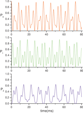
Figure 1: Probabilities of the two-particle Zeeman states in the absence of magnetic field.

In the presence of a magnetic field, the linear and quadratic Zeeman terms should be included into the interaction Hamiltonian sengstock

$$H=V-p(S_{1z}+S_{2z})+q(S_{1z}^{2}+S_{2z}^{2}),$$ (6)

where $p=\mu_{B}B/2\hbar$, the ground state hyperfine splitting $\omega_{hfs}\approx 2\pi\times 6.835GHz$ for ⁸⁷Rb atoms, and $q=p^{2}/\omega_{hfs}\approx 450B^{2}Hz/G^{2}$. In this case, the total spin angular momentum is no longer conserved, but its z-component is still conserved. Therefore, we can work in the subspace of $m_{1}+m_{2}=0$, in which the second order Zeeman shift can influence the spin dynamics. In the complete bases of $\left|0,0\right\rangle$, $\left|1,-1\right\rangle$, and $\left|2,-2\right\rangle$, the effective Hamiltonian could be expressed as:

$$H_{eff}=\left[\begin{array}[]{ccc}9.82J&7.02J&-0.05J\\ 7.02J&8.15J+2q&3.35J\\ -0.05J&3.35J&3.22J+8q\end{array}\right],$$ (7)

where we have used $a_{0}=89.4a_{B}$, $a_{2}=94.5a_{B}$, and $a_{4}=106.0a_{B}$ for ⁸⁷Rb atoms ciobanu , and $J=\frac{4\pi\hbar^{2}n^{2}}{M}\int\mathbf{dr}\left|\varphi\right|^{4}$ is typically chosen as $129.02Hz$. To solve this Hamiltonian, one has to employ the numerical method. Using the harmonic wave function to approximate $\varphi$, one could estimate

$$Ja_{B} \sim \frac{a_{B}\hbar^{2}}{\pi M}\sqrt{\frac{2}{\pi}}(\frac{k}{\hbar}\sqrt{2V_{0}M})^{3/2}$$ (8)

$$= 4.08v^{3/4}Hz,$$

where $V_{0}=v\frac{\hbar^{2}k^{2}}{2M}$ is the depth of the lattice potential. In the Mott insulating regime, $v$ is large and we simply choose $v=100$. In Fig.2a, the eigenvalues of the effective Hamiltonian ($\overset{\_}{E}_{1}>\overset{\_}{E}_{2}>\overset{\_}{E}_{3}$) have been presented as a function of the magnetic field.

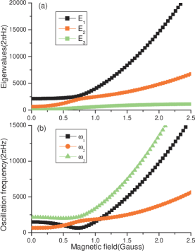
Figure 2: Eigenvalues of the effective model in (a) and the corresponding three oscillation frequencies in (b) as a function of magnetic field.

In the presence of the second order Zeeman shift, three two-particle Zeeman states can still be expressed in terms of three eigenstates

$$\left|0,0\right\rangle = U_{11}\left|\overset{\_}{E}_{1}\right\rangle+U_{12}\left|\overset{\_}{E}_{2}\right\rangle+U_{13}\left|\overset{\_}{E}_{3}\right\rangle,$$

$$\left|1,-1\right\rangle = U_{21}\left|\overset{\_}{E}_{1}\right\rangle+U_{22}\left|\overset{\_}{E}_{2}\right\rangle+U_{23}\left|\overset{\_}{E}_{3}\right\rangle,$$

$$\left|2,-2\right\rangle = U_{31}\left|\overset{\_}{E}_{1}\right\rangle+U_{32}\left|\overset{\_}{E}_{2}\right\rangle+U_{33}\left|\overset{\_}{E}_{3}\right\rangle,$$ (9)

where nine coefficients are calculated numerically and are plotted as a function of the magnetic field in Fig.3a. It can be seen that $U_{11}$ and $U_{33}\,$become very small and reduce quickly to zero as the magnetic field is increased. When $U_{11}=0$, the initial state is just a superposition of two eigenstates only $\left|0,0\right\rangle\simeq U_{12}\left|\overset{\_}{E}_{2}\right\rangle+U_{13}\left|\overset{\_}{E}_{3}\right\rangle$, so it will not jump into third eigenstate $\left|\overset{\_}{E}_{1}\right\rangle$. Similar to the previous procedure, the probabilities of the Zeeman states are obtained as the form of

$$P_{0} = A_{00}+A_{01}\cos\omega_{1}t+A_{02}\cos\omega_{2}t+A_{03}\cos\omega_{3}t,$$

$$P_{1} = A_{10}+A_{11}\cos\omega_{1}t+A_{12}\cos\omega_{2}t+A_{13}\cos\omega_{3}t,$$

$$P_{2} = A_{20}+A_{21}\cos\omega_{1}t+A_{22}\cos\omega_{2}t+A_{23}\cos\omega_{3}t,$$

with the amplitudes as combinations of the coefficients $U_{ij}$

$$A_{00} = U_{11}^{4}+U_{12}^{4}+U_{13}^{4},\,A_{10}=U_{11}^{2}U_{12}^{2}+U_{12}^{2}U_{22}^{2}+U_{13}^{2}U_{23}^{2},\,A_{20}=U_{11}^{2}U_{31}^{2}+U_{12}^{2}U_{32}^{2}+U_{13}^{2}U_{33}^{2},\text{\ \ \ \ }$$

$$A_{01} = 2U_{11}^{2}U_{12}^{2},\text{ \ \ \ \ \ \ \ \thinspace\thinspace}A_{11}=2U_{11}U_{12}U_{21}U_{22},\text{\ \ \ \ \ \ \ \ \ \ \ \ }A_{21}=2U_{11}U_{12}U_{31}U_{32},$$

$$\text{ }A_{02} = 2U_{12}^{2}U_{13}^{2},\,\ \ \ \ \ \ \ \ \,A_{12}=2U_{12}U_{13}U_{22}U_{23},\ \ \ \ \ \ \ \ \ \ \ \ A_{22}=2U_{12}U_{13}U_{32}U_{33},\text{ \ \ }$$

$$\text{\ }A_{03} = 2U_{11}^{2}U_{13}^{2},\text{ \ \ \ \ \ \ \ \thinspace\thinspace}A_{13}=2U_{11}U_{13}U_{21}U_{23},\ \ \ \ \ \ \ \ \ \ \ \ A_{23}=2U_{11}U_{13}U_{31}U_{33},$$ (10)

and the frequencies are given by

$$\omega_{1}=\overset{\_}{E}_{1}-\overset{\_}{E}_{2},\omega_{2}=\overset{\_}{E}_{2}-\overset{\_}{E}_{3},\omega_{3}=\overset{\_}{E}_{1}-\overset{\_}{E}_{3}.$$

There are simple relations between the amplitudes of each oscillations and the frequencies:

$$A_{0n}+A_{1n}+A_{2n}=\delta_{n,0},\text{ \ }\omega_{3}=\omega_{1}+\omega_{2}.$$ (11)

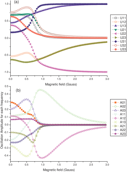
Figure 3: Expansion coefficients of the two-particle Zeeman states in terms of eigenstates $U_{ij}$ in (a) and the amplitudes of each frequency oscillation $A_{ij}$ in (b) as a function of magnetic field.

As the magnetic field $B$ gradually increases, the frequencies $\omega_{i}$ of the spin oscillations are determined by the eigenvalues $\overset{\_}{E}_{n}$, while the amplitudes of each frequency oscillation are determined by the coefficients $U_{ij}$. By focusing on the amplitudes $A_{mn}$ for each oscillation frequency as the functions of the magnetic field shown in Fig.3b, we can clearly demonstrate how the system crossovers from a three-level ($\left|2,-2\right\rangle$, $\left|1,-1\right\rangle$, $\left|0,0\right\rangle$) coherent oscillation without any selection rules into a two-level ($\left|1,-1\right\rangle$, $\left|0,0\right\rangle$) Rabi-like oscillation.

When the large magnetic field is typically larger than $0.8G$, which is a reasonable magnitude compared to the experimental parameters widera-prl , all amplitudes $A_{mn}$ begin to fall quickly down to zero except for $A_{02}$ and $A_{12}$. Thus, $P_{2}(t)$ could be neglected and $P_{0}$ and $P_{1}$ are reduced into an oscillation with a cosine form, i.e., the system oscillates between $\left|0,0\right\rangle$ and $\left|1,-1\right\rangle$ like a Rabi oscillation. In Fig.4, we have plotted the probabilities of the three Zeeman states at $B=1.2G$. To find out the more detailed reason, one must look into the coefficients $U_{ij}$ shown in Fig.3b: $U_{11}$ and $U_{33}\,$become very small and reduce quickly to zero, $A_{m1}$ and $A_{m3}$ ($m=1,2,3)$ including $U_{11}$ fall down to zero, and $A_{22}$ including $U_{33}$ falls down to zero too. In the extreme limit of $q/J\gg 1$, all $U_{ij}$ are zero except $U_{13},\,U_{22,}\,U_{31}$ equal to $1$. Then the initial state $\left|0,0\right\rangle$ just corresponds to one eigenstate, so there will be no spin-exchange collisional dynamics.

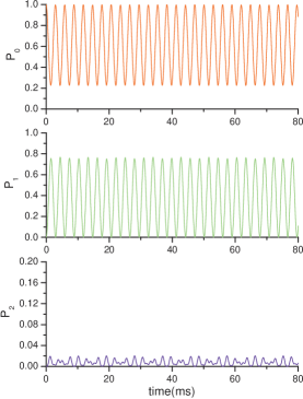
Figure 4: Probabilities of the two-particle Zeeman states in the large magnetic field $B=1.2G$.

However, in the weak magnetic field regime, the amplitudes of three frequencies in $P_{0}$, $P_{1}$ and $P_{2}$ are all finite and comparable, displaying the three-level coherent oscillations. As $B$ is gradually increasing, the different eigenvalues grow with different slopes. Around a critical magnetic field $B_{c}\approx 0.48G$,  $\omega_{1}$ and $\omega_{2}$ are very close to each other, $A_{01}\simeq A_{02}\simeq 0.15$, $\,A_{03}\simeq 0.35$, $\ A_{11}\simeq A_{12}\simeq 0$, $\,A_{13}\simeq-0.42$, $\,A_{21}\simeq A_{22}\simeq-0.15$,  and$\ A_{23}\simeq 0.07$. Since $A_{23}$ is small with compared to the beat amplitude (roughly $2A_{21}$ or $2A_{22}$), there appears a clear quantum beating phenomenon presence in the probability of the Zeeman state $|2,-2\rangle$. Meanwhile, the corresponding probability $P_{0}(t)$ exhibits a combination of a beating oscillation and a sinusoidal one with the frequency $2\omega$, because the sinusoidal amplitude $A_{03}\$is comparable to the beat amplitude (roughly $2A_{01}$ or $2A_{02}$). $P_{1}(t)$ just corresponds to a single frequency oscillation. In Fig.5, we have plotted the three probabilities at $B=0.47G$. Considering that this novel phenomenon is very sensitive to the external magnetic field, the critical point might be accurately determined by fine-tuning the external field experimentally.

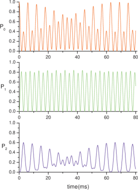
Figure 5: Probabilities of the two-particle Zeeman states at $B=0.47G$ around the critical magnetic field.

In conclusion, we have studied the collisional spin dynamics of an isolated spin-2 ⁸⁷Rb atom pairs confined in a deep optical lattice. Although our calculations could not consider the damping of the oscillations, some clear experimental predictions are given in the weak magnetic field limit, and we have also demonstrated the presence of a crossover from the three-level to two-level coherent spin dynamics. In particular, when the system is initialized as $|0,0\rangle$ and the magnetic field $B_{c}\approx 0.48G$, the probability in the two-particle Zeeman state $|2,-2\rangle$ will exhibit a quantum beat phenomenon, which is ready to be confirmed in future experiments.

The authors are indebted to Prof. Li You for his many stimulating discussions, and G. M. Zhang is supported by NSF-China (Grant No. 10125418 and 10474051).

References

• (1) Tin-Lun Ho, Phys. Rev. Lett. 81, 742 (1998).
• (2) T. Ohmi and K. Machida, J. Phys. Soc. Jpn. 67, 1822 (1998).
• (3) C. K. Law, H. Pu, and N. P. Bigelow, Phys. Rev. Lett. 81, 5257 (1998).
• (4) H. Pu, C. K. Law, and S. Raghavan, J. H. Eberly, and N. P. Bigelow, Phys. Rev. A 60, 1463 (1999).
• (5) C. V. Ciobanu, S. -K. Yip, and Tin-Lun Ho, Phys. Rev. A 61, 033607 (2000).
• (6) M. Koashi and M. Ueda, Phys. Rev. Lett. 84, 1066 (2000); Phys. Rev. A 65, 063602 (2002).
• (7) W. Zhang, D. L. Zhou, M. -S. Chang, M. S. Chapman, L. You, Phys. Rev. A 72, 013602 (2005).
• (8) D. M. Stamper-Kurn and W. Ketterle, in Coherent Matter Waves, edited by R. Kaiser, C. Westbrook, and F. David (Springer, New York, 2001).
• (9) M. D. Barrett, J. A. Sauer, and M. S. Chapman, Phys. Rev. Lett. 87, 010404 (2001).
• (10) H. Schmaljohann, M. Erhard, J. KronjΓ€ger, M. Kottke, S. von Staa, L. Cacciapuoti, J. J. Arlt, K. Bongs, and K. Sengstock, Phys. Rev. Lett. 92, 040402 (2004).
• (11) M. -S. Chang, C. D. Hamley, M. D. Barrett, J. A. Sauer, K. M. Fortier, W. Zhang, L. You, and M. S. Chapman, Phys. Rev. Lett. 92, 140403 (2004).
• (12) T. Kuwamoto, K. Araki, T. Eno, and T. Hirano, Phys. Rev. A 69, 063604 (2004).
• (13) J. M. Higbie, L. E. Sadler, S. Inouye, A. P. Chikkatur, S. R. Leslie, K. L. Moore, V. Savalli, and Stamper-Kurn, Phys. Rev. Lett. 95, 050401 (2005).
• (14) J. KronjΓ€ger, C. Becker, M. Brinkmann, R. Walser, P. Navez, K. Bongs, and K. Sengstock, cond-mat/0509083.
• (15) M. -S Chang, Q. Qin, W. Zhang, L. You and M. S. Chapman, Nature Physics 1, 111 (2005).
• (16) A. Widera, F. Gerbier, S. FΓΆling, T. Gericke, O. Mandel, and I. Bloch, Phys. Rev. Lett. 95, 190405 (2005).