Superfluid-Insulator transitions of bosons on Kagome lattice at non-integer fillings

Abstract

We study the superfluid-insulator transitions of bosons on the Kagome lattice at incommensurate filling factors $f=1/2$ and $2/3$ using a duality analysis. We find that at $f=1/2$ the bosons will always be in a superfluid phase and demonstrate that the $T_{3}$ symmetry of the dual (dice) lattice, which results in dynamic localization of vortices due to the Aharonov-Bohm caging effect, is at the heart of this phenomenon. In contrast, for $f=2/3$, we find that the bosons exhibit a quantum phase transition between superfluid and translational symmetry broken Mott insulating phases. We discuss the possible broken symmetries of the Mott phase and elaborate the theory of such a transition. Finally we map the boson system to a XXZ spin model in a magnetic field and discuss the properties of this spin model using the obtained results.

I Introduction

The superfluid (SF) to Mott insulators (MI) transitions of strongly correlated lattice bosons systems, described by extended Hubbard models, in two spatial dimensions have recently received a great deal of theoretical interest. One of the reasons for this renewed attention is the possibility of experimental realization of such models using cold atoms trapped in optical lattices bloch1 ; kasevitch1 . However, such transitions are also of interest from a purely theoretical point of view, since they provide us with a test bed for exploring the recently developed theoretical paradigm of non-Landau-Ginzburg-Wilson (LGW) phase transitions senthil1 . In the particular context of lattice bosons in two spatial dimensions, a general framework for such non-LGW transitions has been developed and applied to the case of square lattice balents1 . An application of these ideas for triangular lattice has also been carried out burkov1 .

The typical paradigm of non-LGW transitions that has been proposed in the context of lattice bosons in Refs. balents1, and burkov1, is the following. For non-integer rational fillings $f=p/q$ of bosons per unit cell of the underlying lattice ($p$ and $q$ are integers), the theory of phase transition from the superfluid to the Mott insulator state is described in terms of the vortices which are non-local topological excitations of the superfluid phase, living on the dual lattice.fisher1 ; tesanovic1 These vortices are not the order parameters of either superfluid or Mott insulating phases in the usual LGW sense. Thus the theory of the above mentioned phase transitions are not described in terms of the order parameters on either side of the transition which is in contrast with the usual LGW paradigm of phase transitions. Also, as explicitly demonstrated in Ref. balents1, , although these vortices are excitations of a featureless superfluid phase, they exhibit a quantum order which depends on the filling fraction $f$. It is shown that the vortex fields describing the transition form multiplets transforming under projective symmetry group (projective representations of the space group of the underlying lattice). It is found that this property of the vortices naturally and necessarily predicts broken translational symmetry of the Mott phase, where the vortices condense. Since this translational symmetry breaking is dependent on the symmetry group of the underlying lattice, geometry of the lattice naturally plays a key role in determining the competing ordered states of the Mott phase and in the theory of quantum phase transition between the Mott and the superfluid phases.

In this work, we apply the theoretical framework developed in Refs. balents1, to bosons on Kagome lattice described by the extended Bose-Hubbard Hamiltonian

$$H_{\rm boson} = -t\sum_{\left<ij\right>}\left(b_{i}^{\dagger}b_{j}+{\rm h.c.}\right)+\frac{U}{2}\sum_{i}n_{i}\left(n_{i}-1\right)$$ (1)

$$+V\sum_{\left<ij\right>}n_{i}n_{j}-\mu\sum_{i}n_{i}$$

at boson fillings $f=1/2$ and $2/3$. Here $t$ is the boson hopping amplitude between nearest neighbor sites, $U$ is the on-site interaction, $V$ denotes the strength of the nearest neighbor interaction between the bosons and $\mu$ is the chemical potential.

The main motivation of this study is two fold. First, since the geometry of the underlying lattice plays a significant role in determining the nature of the Mott phase, we expect that such phases in Kagome lattice would be distinct from their square balents1 or triangular burkov1 counterparts studied so far. In particular, the dual of the Kagome lattice is the dice lattice which is known to have $T_{3}$ symmetry vidal1 . It is well known that the particles in a magnetic field on such lattice experience a destructive Aharonov-Bohm interference effect at special values of the external magnetic flux leading to dynamic localization of the particles. This phenomenon is termed as Aharonov-Bohm caging in Ref. vidal1, . In the problem at hand, the vortices reside on the dual (dice) lattice and the boson filling $f$ acts as the effective magnetic flux for these vortices. Consequently, we find that at filling $f=1/2$, the vortices become localized within the Aharonov-Bohm cages vidal1 and can never condense. As a result, the bosons always have a featureless superfluid ground state. Such localization of vortices and consequently the absence of a Mott phase for bosons is a direct consequence of the geometry of the Kagome (or it’s dual dice) lattice and is distinctly different from expected and previously studied behaviors of bosons on square or triangular lattices balents1 ; burkov1 whose dual lattices do not have $T_{3}$ symmetry. In contrast, for $f=2/3$, we find that there is a translational symmetry broken Mott phase and discuss the possible competing ordered states in the Mott phase based on the vortex theory at a mean-field level. We also address the question of quantum phase transition from such an ordered state to the superfluid and write down an effective vortex field theory for describing such a transition.

The second motivation for undertaking such a study comes from the interest in physics of XXZ models with ferromagnetic $J_{x}$ and antiferromagnetic $J_{z}$ interaction in a longitudinal magnetic field $B_{l}$

$$H_{\rm XXZ} = -J_{x}\sum_{\left<ij\right>}\left(S_{i}^{x}S_{j}^{x}+S_{i}^{y}S_{j}^{y}\right)+J_{z}\sum_{\left<ij\right>}S_{i}^{z}S_{j}^{z}$$ (2)

$$-B_{l}\sum_{i}S^{z}_{i}$$

where $J_{x}>0$ and $J_{z}>0$ are the strengths of transverse and longitudinal nearest neighbor interactions. Such spin models on Kagome lattice have been widely studied numerically cabra1 ; sergei1 . Further, the large $J_{z}$ limit of this model (in the presence of an additional transverse magnetic field) has also been studied before sondhi1 . A couple of qualitative points emerge from these studies. First, in the absence of external field $B_{l}$, such models on Kagome lattice do not exhibit $S_{z}$ ordering for any values of $J_{z}/J_{x}$. This absence of ordering is an unique property of the Kagome lattice and it has been conjectured that the ground state is quantum disordered.sondhi1 Second, for $B_{l}\neq 0$ and net magnetizations $m=\left<S_{z}\right>=\hbar/6,\hbar/3$, the model exhibit a quantum phase transition between a featureless state with $\left<S_{x}\right>\neq 0$ to a translational symmetry broken ordered state with finite $m$. Using a simple Holstein-Primakoff transformation which maps the $H_{\rm XXZ}$ (Eq. 2) to hardcore Bose-Hubbard model $H_{1}$ (Eq. 4), we show that it is possible to understand both of these features analytically at least at a qualitative level. The absence $S_{z}$ ordering for $B_{l}=0$ (which corresponds to average boson filling $f=1/2$) turns to be a natural consequence of Aharonov-Bohm caging phenomenon discussed earlier. Further, the results from the analysis of the Boson model at $f=2/3$ can also be carried over to study the possible $S_{z}$ orderings of the spin model at net magnetization $\hbar/3$ which allows us to make contact with recent numerical studies in Refs. sergei1, and cabra1, .

The organization of the paper is as follows. In the next section, we map between the spin model $H_{\rm XXZ}$ to an boson model and carry out a duality analysis of this boson model. The dual Lagrangian so obtained is analyzed in Sec. III for both filling factors $f=1/2$ and $2/3$. This is followed by a discussion of the results in Sec. IV. Some details of the calculations are presented in Appendices A, B and C.

II Duality Analysis

To analyze the spin model $H_{\rm XXZ}$, our main strategy is to map it to a Boson model using the well-known Holstein-Primakoff transformation

$$S^{+}_{i}=(S_{i}^{-})^{\ast}\equiv b_{i}\quad S_{i}^{z}\equiv\left(b_{i}^{\dagger}b_{i}-\frac{1}{2}\right)$$ (3)

Such a transformation maps $H_{\rm XXZ}$ to $H_{1}$ given by

$$H_{1} = -t\sum_{\left<ij\right>}\left(b_{i}^{\dagger}b_{j}+{\rm h.c.}\right)$$ (4)

$$+V\sum_{\left<ij\right>}(n_{i}-f)(n_{j}-f)$$

with the hardcore constraint $n_{i}\leq 1$ on each site. The parameters of the hardcore boson model $H_{1}$ are related to those of $H_{\rm XXZ}$ as

$$J_{x} = 2t,\quad J_{z}=V,\quad B_{l}=zV\left(f-\frac{1}{2}\right)$$ (5)

where $z$ is the boson coordination number. In the Mott phases, the average boson density is locked to some number and this will be $f$ in Eqs.4 and 5. In this work, we will consider the superfluid-insulator transitions with the average boson density fixed across the transition.

In what follows, we would carry out a duality analysis of the hardcore boson model. Such a duality analysis of the boson model is most easily done by imposing the hardcore constraint in $H_{1}$ (Eq. 4) by a strong on-site Hubbard term potential to obtain $H_{\rm boson}$ (Eq. 1). In the limit of strong U the qualitative nature of the phases of the model is expected to be the same as that of the hardcore model. Hence for rest of the work, we shall consider the boson model $H_{\rm boson}$. Also, since we are going to carry out a duality analysis of this model, we shall not bother about precise relations between parameters of $H_{1}$ and $H_{\rm boson}$, but merely represent $\mu$ to be a chemical potential which forces a fixed filling fraction $f$ of bosons as shown in previous work balents1 .

The dual representation of $H_{\rm boson}$ can be obtained in the same way as in Refs. balents1, ; burkov1, . The details of the duality transformation are briefly sketched in Appendix A. The dual theory turns out to be a theory of U(1) vortices, residing on the sites of the dual (dice) lattice shown in Fig. 1, coupled to a fictitious magnetic field which depends on the boson filling $f$. The dual action is given by

$$S_{d} = \frac{1}{2e^{2}}\sum_{p}\left(\epsilon_{\mu\nu\lambda}\Delta_{\nu}A_{b\lambda}-f\delta_{\mu\tau}\right)^{2}$$ (6)

$$-y_{v}\sum_{b,\mu}\left(\psi_{b+\mu}^{\dagger}e^{2\pi iA_{b\mu}}\psi_{b}+{\rm h.c}\right)$$

$$+\sum_{b}r|\psi_{b}|^{2}+u|\psi_{b}|^{4}+....$$

where $\psi_{b}$ are the vortex field living on the site $b$ of the dual (dice) lattice, $A_{b\mu}$ is the U(1) dual gauge field so that $\epsilon_{\tau\nu\lambda}\Delta_{\nu}A_{b\lambda}=n_{i}$ where $n_{i}$ is the physical boson density at site $i$, $\sum_{p}$ denotes sum over elementary rhombus of the dice lattice$,\Delta_{\mu}$ denotes lattice derivative along $\mu=x,y,\tau$, and $f$ is the average boson density. The magnetic field seen by the vortices is therefore the physical boson density. Note that the vortex action $S_{d}$ is not self-dual to the boson action obtained from $H_{\rm boson}$. Therefore we can not, in general, obtain a mapping between the parameters of the two actions, except for identifying $\epsilon_{\tau\nu\lambda}\Delta_{\nu}A_{b\lambda}$ as the physical boson density balents1 ; burkov1 . Therefore, in the remainder of the paper, we shall classify the phases of this action based on symmetry consideration and within the saddle point approximation as done in Ref. balents1, .

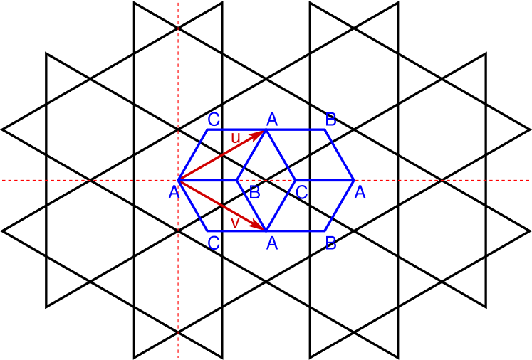
Figure 1: Kagome lattice (thin black line) and the unit cell of its dual dice (thick blue lines) lattice. The three inequivalent sites $A$, $B$ and $C$ of the dice lattice are shown in the figure. The sides of the rhombus $ABAC$ have length $a$ and angles $\pi/3$. The basis vectors ${\bf u}=(3a/2,\sqrt{3}a/2)$ and ${\bf v}=(3a/2,-\sqrt{3}a/2)$ that span the dice lattice are shown as arrowed lines. Note that the $A$ sides reside in the center of the hexagons of the Kagome lattice while the $B$ and $C$ sites reside in the center of the triangles.

The transition from a superfluid ($\left<\psi_{b}\right>=0$) to a Mott insulating phase in $S_{d}$ can be obtained by tuning the parameter $r$. For $r>0$, we are in the superfluid phase. Note that the saddle point of the gauge fields $A_{b\mu}$ in action corresponds to $\epsilon_{\tau\nu\lambda}\Delta_{\nu}{\bar{A}}_{b\lambda}=f$, so that the magnetic field seen by the vortices is pinned to the average boson filling $f$. Now as we approach the phase transition point $r=0$, the fluctuations about this saddle point ($\left<\psi_{b}\right>=0$, ${\bar{A}}_{by}=fx$) increase and ultimately destabilize the superfluid phase in favor of a Mott phase with $\left<\psi_{b}\right>\neq 0$. Clearly, in the above scenario, the most important fluctuations of the vortex field $\psi_{b}$ are the ones which has the lowest energy. This prompts us to detect the minima of the vortex spectrum by analyzing the kinetic energy term of the vortices

$$H_{\rm kinetic} = -y_{v}\sum_{b,\alpha}\left(\psi_{b+\alpha}^{\dagger}e^{2\pi i{\bar{A}}_{b}}\psi_{b}+{\rm h.c}\right)$$ (7)

where the sum over $\alpha$ is carried out over the six-fold (for $A$ sites in Fig. 1) or three-fold (for $B$ and $C$ sites) coordinated sites surrounding the site $b$.

The analysis of $H_{\rm kinetic}$ amounts to solving the Hofstadter problem on the dice lattice which has been carried out in Ref. vidal1, . We shall briefly summarize the relevant part of that analysis. It is found that the secular equation obtained from $H_{\rm kinetic}$ for boson filling factor $f$ is given by vidal1

$$\epsilon\psi_{A}(x,\kappa) = \psi_{B}(x+a)+\psi_{C}(x-a)$$

$$+2\cos\left[\frac{\gamma}{a}\left(x-a/4\right)+\kappa\right]\psi_{B}(x-a/2)$$

$$+2\cos\left[\frac{\gamma}{a}\left(x+a/4\right)+\kappa\right]\psi_{C}(x+a/2)$$

$$\epsilon\psi_{B}(x,\kappa) = \psi_{A}(x-a)$$

$$+2\cos\left[\frac{\gamma}{a}\left(x+a/4\right)+\kappa\right]\psi_{A}(x+a/2)$$

$$\epsilon\psi_{C}(x,\kappa) = \psi_{A}(x-a)$$ (8)

$$+2\cos\left[\frac{\gamma}{a}\left(x-a/4\right)+\kappa\right]\psi_{A}(x-a/2)$$

where $A$, $B$ and $C$ denote inequivalent sites of the dice lattice, $\gamma=2\pi f=2\pi\phi/\phi_{0}$ for the boson filling $f$, and $\phi$ is the dual flux through an elementary rhombus of the lattice. Here $\psi=(\psi_{A},\psi_{B},\psi_{C})$ is the vortex wavefunction which has been written as $\psi_{b}\equiv\psi(x,y)=\psi(x,\kappa)\exp(i\kappa n)$ with $\kappa={\sqrt{3}}k_{y}a/2$ and integer $n=2y/(\sqrt{3}a)$, a is the lattice spacing of the dice lattice, and $\epsilon$ is the energy in units of vortex fugacity $y_{v}$. For obtaining the solutions corresponding to $\epsilon\neq 0$, we eliminate for $\psi_{B}$ and $\psi_{C}$ from Eq. 8 to arrive at an one-dimensional equation for $\psi_{A}(x=3ma/2,\kappa)\equiv\psi_{A}(m,\kappa)$

$$\left(\frac{\epsilon^{2}-6}{2\cos\left(\gamma/2\right)}\right)\psi_{A}(m,\kappa)=2\cos\left(3\gamma m+2\kappa\right)\psi_{A}(m,\kappa)$$

$$+2\cos\left[\frac{3\gamma}{2}\left(m-1/2\right)+\kappa\right]\psi_{A}(m-1,\kappa)$$

$$+2\cos\left[\frac{3\gamma}{2}\left(m+1/2\right)+\kappa\right]\psi_{A}(m+1,\kappa)$$ (9)

where we have used the fact that with our choice of origin the $A$ sites have $x=3ma/2$ with integer $m$. For rational boson filling $f=p/q$, Eq. 9 closes after translation by $q$ periods. However, for $q=3q^{\prime}\,[q^{\prime}\in{\rm integer}]$, this periodicity is reduced to $q^{\prime}$ vidal1 .

A key feature of the wavefunction $\psi$ that we would be using in the subsequent analysis is its transformation property under all distinct space group operations of the dice lattice. Therefore we collect all such transformations here for any general filling $f$. Such operations for the dice lattice, as seen from Fig. 1, involve translations $T_{u}$ and $T_{v}$ along vectors $u=(3a/2,{\sqrt{3}}a/2)$ and $v=(3a/2,-{\sqrt{3}}a/2)$, rotations $\pi n/3$ for any integer n, and reflection $I_{x}$ about the $x$ axis. It is easy to check that these are the basic symmetry operations that must leave the Hamiltonian invariant and all other symmetry operations can be generated by their appropriate combinations. Following methods outlined in Ref. balents1, , one finds the following transformation properties for the wavefunctions:

$$T_{\alpha=u,v}:\psi(x,y)\rightarrow\psi(x-\alpha_{x},y-\alpha_{y})\omega^{\alpha_{x}y2/\sqrt{3}}$$ (10)

$$I_{x}:\psi(x,y)\rightarrow\psi^{\ast}(x,-y)$$ (11)

$$R_{\pi/3}:\psi_{A}(x,y)\rightarrow\psi_{A}\left([x+\sqrt{3}y]/2,[y-\sqrt{3}x]/2\right)$$

$$\times\omega^{\left[\left(y^{2}-x^{2}\right)/4+\sqrt{3}xy/2\right]}$$

$$\psi_{B}(x,y)\rightarrow\psi_{C}\left([x+\sqrt{3}y]/2,[y-\sqrt{3}x]/2\right)$$

$$\times\omega^{\left[\left(y^{2}-x^{2}\right)/4+\sqrt{3}xy/2\right]}$$

$$\psi_{C}(x,y)\rightarrow\psi_{B}\left([x+\sqrt{3}y]/2,[y-\sqrt{3}x]/2\right)$$

$$\times\omega^{\left[\left(y^{2}-x^{2}\right)/4+\sqrt{3}xy/2\right]}$$ (12)

where $(x,y)$ are the coordinates of the dice lattice and $\omega=\exp(2\pi if)$, Here $\psi$ may denote either $\psi_{A}(x=3ma/2,y=\sqrt{3}na/2)$ or $\psi_{B}$ and $\psi_{C}$ at appropriate positions within the unit cell. Note that all other above mentioned symmetry operations can be generated by combination of the operations listed in Eqs. 10..12. For example $I_{y}=I_{x}R_{\pi}=I_{x}R_{\pi/3}^{3}$ and under this transformation $\psi_{A}(x,y)\rightarrow\psi_{A}^{\ast}(-x,y)$ and $\psi_{B,C}(x,y)\rightarrow\psi_{C,B}^{\ast}(-x,y)$. Some details of the algebra leading to Eqs. 10..12 is sketched in Appendix B.

In what follows, we are going to analyze the vortex theory for $f=1/2$ and $f=2/3$ which turns out to be the simplest possible physically interesting fractions to analyze.

III Phases for $f=1/2$ and $2/3$

III.1 f=1/2

The key difference between square and triangular lattices analyzed previously balents1 ; burkov1 and the Kagome lattice studied in this work, comes out when we study the filling fraction $f=1/2$. From Eq. 9, we find that for $f=1/2$, $\gamma=\pi$, so that the entire spectrum collapses into three infinitely degenerate bands $\epsilon=0,\pm\sqrt{6}$. This situation is in sharp contrast to the square or the triangular lattices where the vortex spectrum for rational boson fillings $f=p/q$ has a fixed number of well defined minima. It is possible that vortex-vortex interaction may make the degeneracy finite, but it is unlikely to be lifted completely by interaction vidal1 . Therefore the vortex band has zero or at least extremely small bandwidth with no well-developed minima at any wavevector which implies that the vortices shall never condense comment1 . Consequently, we do not expect to have a Mott insulating state at $f=1/2$, as seen in previous Monte Carlo studies $H_{1}$ on Kagome lattice sergei1 . Comparing the parameters of $H_{1}$ and $H_{\rm XXZ}$ (Eq. 5), we find that such an absence of Mott phase also implies that XXZ models on Kagome lattice will have no $S_{z}$ ordering for $B_{l}=0$. This result was also obtained by numerical study of the related transverse field Ising model on the Kagome latticesondhi1 .

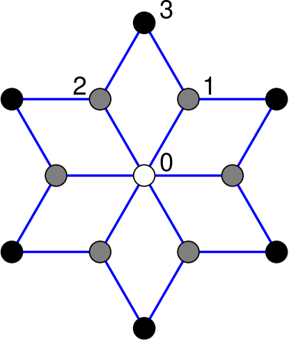
Figure 2: Aharonov-Bohm cage for a vortex on site $0$ of the dice lattice. The probability amplitude for the particle to be at $3$ vanishes due to destructive interference between amplitudes from the paths $0\rightarrow 1\rightarrow 3$ and $0\rightarrow 2\rightarrow 3$. Consequently the vortex can never propagate beyond the rim of the cage (black circles) and is dynamically localized. Analogous cages can be constructed for vortices on sites $B$ and $C$ vidal1 .

Physically, the collapse of the vortex spectrum into three degenerate bands can be tied to localization of the vortex within the so-called Aharonov-Bohm cages as explicitly demonstrated in Refs. vidal1, . An example of such a cage is shown in Fig. 2. A vortex whose initial wavepacket is localized at the central (white) $A$ site can never propagate beyond the black sites which form the border of the cage. This can be understood in terms of destructive Aharonov-Bohm interference: The vortex has two paths $0\rightarrow 1\rightarrow 3$ and $0\rightarrow 2\rightarrow 3$ to reach the rim site $3$ from the starting site $0$. The amplitudes from these paths destructively interfere for $f=1/2$ to cancel each other and hence the vortex can never propagate beyond the rim of the cage. Similar cages can be constructed for vortices with initial wavepacket at sites $B$ and $C$ vidal1 . This dynamic localization of the vortex wavepackets in real space, demonstrated and termed as Aharonov-Bohm caging in Ref. vidal1, , naturally leads to spreading of the vortex wavepacket in momentum space. Hence the vortex spectrum has no well-defined minima at any momenta leading to the absence of vortex condensation.

The question naturally arises regarding the nature of the boson ground state at $f=1/2$ (or equivalently ground state of XXZ model at $B_{l}=0$ and $J_{z}\gg J_{x}$). The dual vortex theory studied here can only predict the absence of vortex condensation due to dynamic localization of the vortices leading to persistence of superfluidity (or $S_{x}$ ordering for XXZ model) at all parameter values. Beyond this, numerical studies are required to discern the precise nature of the state. Previous studies of the transverse Ising model, which is related to the XXZ model, in Ref. sondhi1, have conjectured this state to be a spin liquid state. However, the Monte Carlo studies of the XXZ modelsergei1 did not find any sign of spin liquid state.

III.2 f=2/3

In contrast to $f=1/2$, the physics for $f=2/3$ (or $f=1/3$) turns out to be quite different. In this case, we do not have any dynamic localization effect and the vortex spectrum has well defined minima. Note that for $f=2/3$, Eq. 9 closes after one period and the magnetic Brillouin zone becomes identical to the dice lattice Brillouin zone without a magnetic field vidal1 . As a result, Eq. 9, admits a simple analytical solution

$$\epsilon = -\left(6-2\cos\left(2\kappa\right)+4\cos\left(\kappa\right)\cos(k_{m})\right)^{1/2}$$

$$\psi_{A}(x,y) = \exp\left(im3k_{x}a/2+\kappa n\right)$$ (13)

where we have $\kappa\in(0,\pi)$ and $k_{x}\in(0,4\pi/3)$, and $k_{m}=3k_{x}a/2$. The spectrum has two minima in the magnetic Brillouin zone at $(k_{x}a,\kappa)=(0,\pi/3)\,{\rm and}\,(2\pi/3,2\pi/3)$. The eigenfunctions $\psi=\left(\psi_{A},\psi_{B},\psi_{C}\right)$ , corresponding to these two minima can be obtained from Eqs. 13 and 8. They are

$$\psi_{1} = \exp(i\pi n/3)(c,-c,0)$$

$$\psi_{2} = \exp\left[\frac{2\pi in}{3}+i\pi m\right](c,0,-c)$$ (14)

where $c$ is a normalization constant. Thus the low energy properties of the vortex system can then be characterized in terms of the field $\Phi$:

$$\Phi = \psi_{1}({\bf x})\varphi_{1}({\bf x},t)+\psi_{2}({\bf x})\varphi_{2}({\bf x},t)$$ (15)

where $\varphi_{1(2)}$ are fields representing low energy fluctuations about the minima $\psi_{1(2)}$. As shown in Ref. balents1, , the transition from the superfluid to the Mott phase of the bosons can be understood by constructing a low energy effective action in terms of the $\varphi$ fields.

To obtain the necessary low energy Landau-Ginzburg theory for the vortices, we first consider transformation of the vortex fields $\varphi$ under the symmetries of the dice lattice. Using Eqs. 10,11,12, 14, and 15, one gets

$$T_{u}:\varphi_{1}\rightarrow\varphi_{1}\exp(-i\pi/3)\quad\varphi_{2}\rightarrow\varphi_{2}\exp(i\pi/3)$$

$$T_{v}:\varphi_{1}\rightarrow\varphi_{1}\exp(i\pi/3)\quad\varphi_{2}\rightarrow\varphi_{2}\exp(-i\pi/3)$$

$$I_{x}:\varphi_{1(2)}\rightarrow\varphi^{\ast}_{1(2)}$$

$$I_{y}:\varphi_{1(2)}\rightarrow\varphi^{\ast}_{2(1)}$$

$$R_{2\pi/3}:\varphi_{1(2)}\rightarrow\varphi_{1(2)}$$

$$R_{\pi/3}:\varphi_{1(2)}\rightarrow\varphi_{2(1)}$$ (16)

Some details of the algebra leading to Eq. 16 is given in App. C. It is also instructive to write the two fields $\varphi_{1}$ and $\varphi_{2}$ as two components of a spinor field $\chi=(\varphi_{1},\varphi_{2})$. The transformation properties of $\chi$ can then be written as

$$T_{u}:\chi\rightarrow\chi\exp(-i\tau_{z}\pi/3)$$

$$T_{v}:\chi\rightarrow\chi\exp(i\tau_{z}\pi/3)$$

$$I_{x}:\chi\rightarrow\chi^{\ast}$$

$$I_{y}:\chi\rightarrow\tau_{x}\chi^{\ast}$$

$$R_{2\pi/3}:\chi\rightarrow\chi$$

$$R_{\pi/3}:\chi\rightarrow\tau_{x}\chi$$ (17)

where $\tau_{x,y,z}$ are the usual Pauli matrices. Note that $R_{2\pi/3}$ plays the role of identity here where $R_{\pi/3}$ mixes the two components of the spinor field $\chi$.

The simplest Landau-Ginzburg theory for the vortex fields which respects all the symmetries is

$$L_{v} = L_{v}^{(2)}+L_{v}^{(4)}+L_{v}^{(6)}$$ (18)

$$L_{v}^{(2)} = \sum_{\alpha=1,2}\left[\left|\left(i\partial_{\mu}-eA_{\mu}\right)\varphi_{\alpha}\right|^{2}+r\left|\varphi_{\alpha}\right|^{2}\right]$$ (19)

$$L_{v}^{(4)} = u\left(\left|\varphi_{1}\right|^{4}+\left|\varphi_{2}\right|^{4}\right)+v\left|\varphi_{1}\right|^{2}\left|\varphi_{2}\right|^{2}$$ (20)

$$L_{v}^{(6)} = w\left[\left(\varphi_{1}^{\ast}\varphi_{2}\right)^{3}+{\rm h.c.}\right]$$ (21)

The above lagrangian density can also be written in terms of the $\chi$ fields. In particular the sixth order term becomes $L_{v}^{6}w\left[\sum_{a=\pm}\left(\chi^{\ast}\tau_{a}\chi\right)^{3}\right]$. This turns out to be the lowest-order term which does not commute with $\tau_{z}$ and breaks the $U(1)$ symmetry associated with the relative phase of the bosons. A simple power counting shows that $L_{v}^{(6)}$ is marginal at tree level. Unfortunately, the relevance/irrelevance of such a term beyond the tree level, which is of crucial importance for the issue of deconfinement at the quantum critical point, is not easy to determine in the present context for two reasons. First, the standard $\epsilon$ and large $N$ expansions does not yield reliable results for $2+1$D field theories, at least for $N=2$ which is the case of present interest chen1 . Second, while it is known from numerical studies that such a cubic anisotropy term is relevant for the single vortex species case (for XY transitions in $2+1$ D), the situation remains far less from clear for the two vortex case ashvin1 . We have not been able to determine the relevance/irrelevance of this term in the present work.

If it so turns out that $L_{v}^{(6)}$ is irrelevant, the situation here will be identical to that of bosons on square lattice at $f=1/2$. The relative phase of the vortices would emerge as a gapless low energy mode at the critical point. The quantum critical point would be deconfined and shall be accompanied by boson fractionalization balents1 . On the other hand, if $L_{v}^{(6)}$ is relevant, the relative phase degree of the bosons will always remain gapped and there will be no deconfinement at the quantum critical point. Here there are two possibilities depending on the sign of $u$ and $v$. If $u,v<0$ and $w>0$, the transition may become weakly first order whereas for $u>0$, it remains second order (but without any deconfinement). The distinction between these scenarios can be made by looking at the order of the transition and the critical exponents in case the transition turns out to be second order senthil1 .

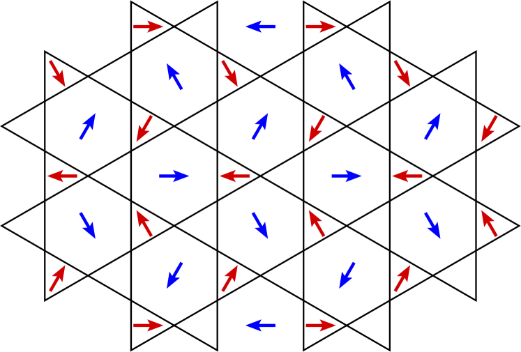
Figure 3: Mean-field vortex state for $v>0$ with $\varphi_{1}\neq 0$. The arrows denote the phase of the vortex wavefunctions $\Phi$ at the sites of the dual lattice. Note that all the sites of the Kagome lattice see the same vortex environment and are therefore equivalent. Hence we do not expect a density wave at the mean-field level.

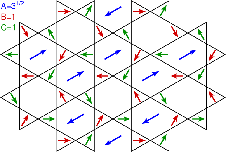
Figure 4: Mean-field vortex state for $v<0$ with $|\varphi_{1}||\varphi_{2}|=1$ and $\theta_{\rm relative}=\pi/3$. The notations are same as in Fig. 3. The magnitudes of the vortex wavefunctions are listed on the left, and $A$, $B$ and $C$ refers to corresponding inequivalent sites of the dual (dice) lattice where the vortices reside. Here there are six inequivalent sites for the Kagome lattice which are listed in Fig. 6.

The vortices condense for $r<0$ signifying the onset of the Mott state and now we list the possible Mott phases. Our strategy in doing so would to be list the sites on the Kagome lattice which sees identical vortex environments (within mean-field) and then obtain the possible ground states based on this classification for a fixed boson filling $f=2/3$. We would like to stress that these results are obtained within mean-field theory without taking into account quantum fluctuations.

First let us consider the case $v>0$. Here only one of the vortex fields condense and consequently the Mott state breaks the symmetry between $B$ and $C$ sites of the dual (dice) lattice. A plot of the mean-field vortex wavefunction for $\left<\varphi_{1}\right>\neq 0$ is shown in Fig. 3. The direction of the arrows denote the phase of the vortex wavefunction at the sites of the dual lattice while the amplitude of the wavefunctions are listed in the figures. We find that for this state all the sites of the Kagome lattice see identical vortex environment and consequently, within mean-field theory, we do not expect density-wave ordering for the bosons. However, the up and down triangles have different vortex environments and one would therefore expect increased effective kinetic energy of the bosons around either the up or down triangles. Consequently one expects an equal superposition state of bosons in which there is equal amplitude of the bosons in the sites around the up(down) triangles balents1 .

For $v<0$, both the vortex fields have non-zero amplitude ${\it i.e.}$ $|\varphi_{1}|=|\varphi_{2}|\neq 0$, and the ground state does not distinguish between the $B$ and the $C$ sites of the dice lattice. The relative phase between the vortex fields is fixed by $L_{v}^{(6)}$:

$$\theta_{\rm relative} = 2\pi p/3\quad{\rm for}\,\,w<0$$ (22)

$$= \pi(2p+1)/3\quad{\rm for}\,\,w>0$$

for integer $p$. The plot of the vortex mean-field wavefunctions are shown in Figs. 5 for $w>0$ and Fig. 6 for $w<0$. The corresponding inequivalent sites, for $w>0$, are charted in Fig. 7. We find that there are six inequivalent sites (defined as those seeing a different vortex environment) in the Kagome lattice. We now aim to construct different density wave patterns based on two rules: a) the boson filling must be $f=2/3$ and b) the equivalent sites shown in Fig. 6 must have the same filling throughout the latticecommentden .

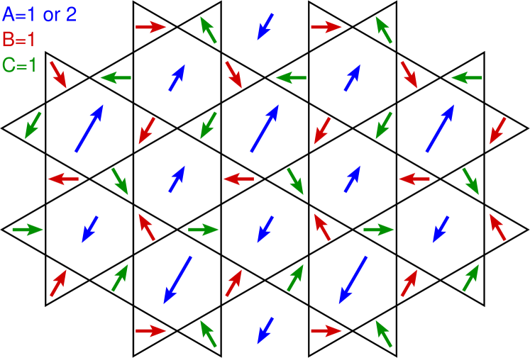
Figure 5: Mean-field vortex state for $v<0$ with $|\varphi_{1}||\varphi_{2}|=1$ and $\theta_{\rm relative}=2\pi/3$. This state also has six inequivalent sites. Notations are same as in Fig. 4.

Such possible states are sketched in Figs. 7 and 8. The state denoted by $\Phi_{1}$ is shown in Fig. 7 and has a $3$ by $3$ ordering pattern. Here all the red and blue sites are empty (or spin down ) while the black and the green sites (both open and closed circles) are occupied (spin up sites). The numbers in the center of the hexagons denote the sum of magnetization (in units of $\hbar/2$) of the sites surrounding the hexagons. For the state $\Phi_{1}$ shown in Fig. 7, these take values $0$ and $6$.

More complicated states $\Phi_{2}$ and $\Phi_{3}$ with $9$ by $9$ ordering pattern are also possible. These are shown in Fig. 8. For the state $\Phi_{2}$ the bosons are localized in red, blue, green (closed circle) and black (open circle) sites whereas the green (open circle) and black (closed circle) sites are vacant. The net magnetization of hexagons for $\Phi_{2}$ takes values $0$, $4$ and $2$ as shown in Fig. 8. The state $\Phi_{3}$ can be similarly obtained from $\Phi_{2}$ by interchanging the occupations of the black and green sites while leaving the red and the blue sites filled. This has the effect of $2\leftrightarrow 4$ for the magnetization of the hexagons. Interestingly, any linear combinations of $\Phi_{2}$ and $\Phi_{3}$, $\Phi(\theta)=\cos(\theta)\Phi_{2}+\sin(\theta)\Phi_{3}$ for any arbitrary mixing angle $\theta$, is also a valid density wave ordered state. The most interesting among these states turn out to be the $\Phi(\pi/4)$ which has an $3$ by $3$ ordering pattern. Such a state corresponds a superposition of filled and empty boson sites on the green and black (both empty and filled) sites whereas the red and blue sites are filled. Here the sum of boson fillings of the sites surrounding the hexagons, takes values $0$ and $3$ as can be inferred from Fig. 8. Notice that the two states $\Phi_{1}$ and $\Phi(\pi/4)$ constructed here has the same long-range ordering pattern.

To distinguish between the states $\Phi_{1}$ and $\Phi(\pi/4)$, consider the operator ${\mathcal{N}}_{b}=\sum_{i\in{\rm hexagon}}n_{i}$, where $\left<{\mathcal{N}}_{b}\right>$ gives the sum of boson fillings of the sites surrounding the hexagon with center $b$. The values of $\left<{\mathcal{N}}_{a}\right>$ for different states has been shown in Figs. 7 and 8. We note that the distinction between the states $\Phi_{1}$ and $\Phi(\pi/4)$ can be made by computing the values of $\left<\sum_{a}{\mathcal{N}}_{a}{\mathcal{N}}_{a+u}\right>$ which measures the correlation between ${\mathcal{N}}$ operators at sites $a$ and $a+u$ where $u$ is the basis vector for the dice lattice shown in Fig. 1. Deep inside the Mott phase such correlations should vanish for $\Phi_{1}$ while it will remain finite for $\Phi(\pi/4)$. Alternatively, one can also compute the distribution of the hexagons with different values of $\left<{\mathcal{N}}_{a}\right>$ to achieve the same goal sergei1 . Such a distribution, computed in Ref. sergei1, , seems to be consistent with the state $\Phi(\pi/4)$ obtained here.

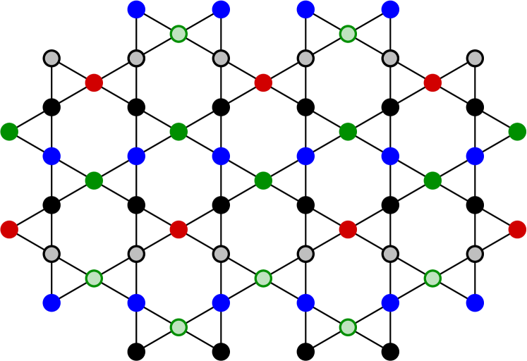
Figure 6: A chart of the inequivalent sites for the mean-field vortex state for $v<0$ with $|\varphi_{1}|=|\varphi_{2}|=1$ and $\theta_{\rm relative}=\pi/3$ denoted by red, blue, green (open and closed) and black (open and closed) circles. Inequivalent sites are defined as those which see a different vortex environment in the surrounding dual lattice. The relevant vortex environments are sketched in Figs. 4 and 5.

Recently exact diagonalization study of XXZ model on Kagome lattice has been carried out in Ref. cabra1, . Their results concluded the existence of $3$ by $3$ patterned RVB state for $m=\hbar/6$. We note that the RVB state proposed in Ref. cabra1, shall have identical long range ordering pattern and $\left<\sum_{a}{\mathcal{N}}_{a}{\mathcal{N}}_{a+u}\right>$ to the state $\Phi(\pi/4)$ obtained in the vortex mean-field theory. Of course, a true RVB state, if it exists, is beyond the reach of the mean-field treatment of the vortex theory. Obtaining such states from a dual vortex analysis is left as an open issue in the present work.

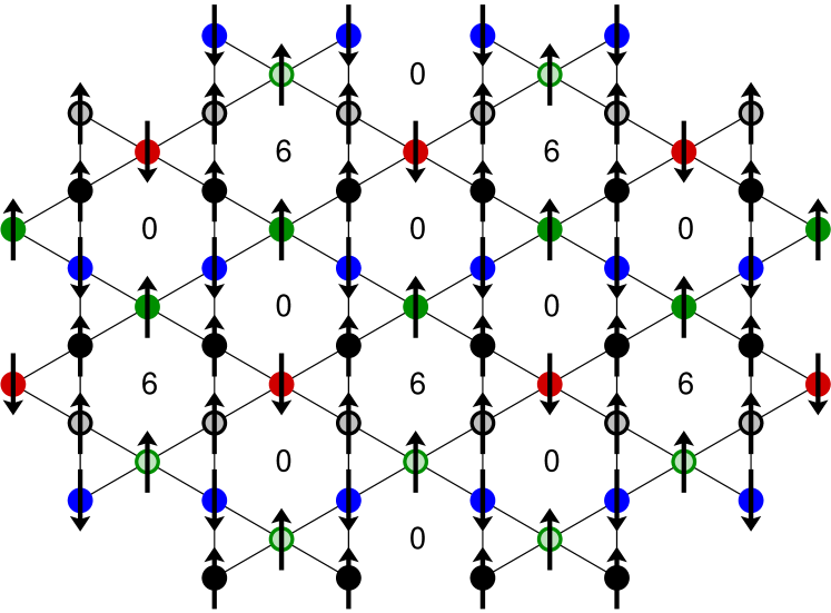
Figure 7: One possible density wave states $\Phi_{1}$ at $f=2/3$ ($m=1/3$ in units of $\hbar/2$) when the black and green (both solid and empty dots) dots have all filled (or spin up) sites while the blue and red sites are empty (spin down). The centers of the hexagons are marked with $6$ and $0$ respectively and shows the sum of magnetization (in units of $\hbar/2$)of the sites surrounding the hexagons. This state shows a $3$ by $3$ density wave pattern as can be seen in the figure. A similar state can be obtained for $f=1/3$ by replacing the bosons with holes and vice versa.

IV Discussion

In this work, we have applied the dual vortex theory developed in Refs. balents1, to analyze the superfluid and Mott insulating phases of extended Bose-Hubbard model (Eq. 1) (or equivalently XXZ model (Eq. 2)) on a Kagome lattice at boson filling $f=1/2,2/3$. The dual theory developed explains the persistence of superfluidity in the bosonic model at $f=1/2$ of arbitrary small values of $t/U,t/V$ seen in the recent Monte-Carlo studies sergei1 , and shows that dynamic localization of vortices due to destructive Aharonov-Bohm interference, dubbed as “Aharonov-Bohm caging” in Ref. vidal1, , is at the heart of this phenomenon. This also offers an explanation of the absence of $S_{z}$ ordering in the XXZ model at zero longitudinal magnetic field for arbitrarily large $J_{z}/J_{x}$ as noted in earlier studies sondhi1 . In contrast for $f=2/3$, we find that there is a direct transition from the superfluid to a translational symmetry broken Mott phase. We have derived a Landau-Ginzburg action in terms of the dual vortex and gauge fields to describe this transition. We have shown that the order and the universality class of the transition depends on relevance/irrelevance of the sixth order term in the effective action. In particular, if this term turns out to be irrelevant, the critical point is deconfined and is accompanied with boson fractionalization. We have also sketched, within saddle point approximation of the vortex action, the possible ordered Mott states that exhibit a $3$ by $3$ ordering pattern. The results obtained here are in qualitative agreement with earlier numerical studies sergei1 ; sondhi1 on related models.

We thank R. Melko and S. Wessel for helpful discussions and collaborations on a related project. We are also grateful to T. Senthil and A. Vishwanath for numerous insightful comments. This work was supported by the NSERC of Canada, Canada Research Chair Program, the Canadian Institute for Advanced Research, and Korea Research Foundation Grant No. KRF-2005-070-C00044.

Noted Added: While this manuscript is being prepared, we became aware of a related work by L. Jiang and J. Ye jiang1 .

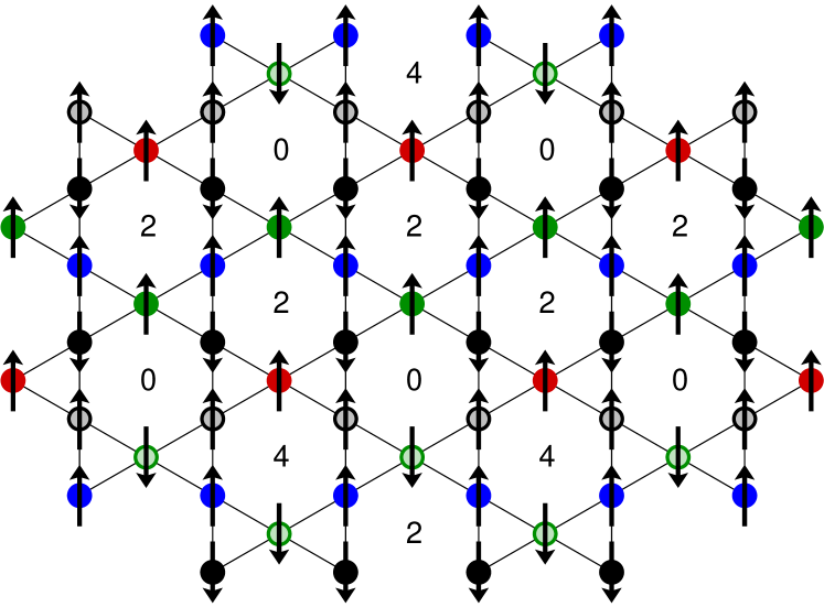
Figure 8: Density wave state $\Phi_{2}$ at $f=2/3$. Here the hexagons with black and green (both solid and open circles) dots have net boson filling $3$ (or magnetization $0$ in spin language). The blue and red sites are filled (spin up). The centers of the hexagons are marked with $0$, $2$ and $4$ respectively and reflects the sum of magnetization of the sites surrounding the hexagons. This state shows a $9$ by $9$ density wave pattern (full pattern not shown in the figure). Another state $\Phi_{3}$ with the same periodicity is easily obtained from $\Phi_{2}$ by simply reversing the direction of the spins (or changing from being filled to being empty and vice versa) on all the green and the black sites (both open and solid black and green circles) while leaving the blue and the red sites unchanged. This has the effect of $2\leftrightarrow 4$ for the magnetization of the hexagons. Note that any linear superposition $\Phi(\theta)=\cos(\theta)\Phi_{2}+\sin(\theta)\Phi_{3}$ is also a possible ground state with $\left<m\right>=1/3$. The state $\Phi(\pi/4)$ has a periodicity of $3$ by $3$.

Appendix A Duality transformation

In this section, we briefly sketch the duality analysis which leads to the dual action (Eq. 6). We start from the Bose-Hubbard model $H_{\rm boson}$ (Eq. 1). First, we follow Ref. steve1, , to obtain an effective rotor model from $H_{\rm boson}$ given by

$$H_{\rm rotor} = -t\sum_{\left<i\alpha\right>}\cos\left(\Delta_{\alpha}{\hat{\phi}}_{i}\right)+V\sum_{\left<ij\right>}{\hat{n}}_{i}{\hat{n}}_{j}$$ (23)

$$+\sum_{i}\left[-\mu{\hat{n}}_{i}+\frac{U}{2}{\hat{n}}_{i}\left({\hat{n}}_{i}-1\right)\right]$$

where the rotor phase (${\hat{\phi}}$) and number (${\hat{n}}$) operators satisfy the canonical commutation relation $\left[{\hat{\phi}}_{i},{\hat{n}}_{j}\right]=i\delta_{ij}$, $\Delta_{\alpha}$ denotes lattice derivative such that $\Delta_{\alpha}{\hat{\phi}}_{i}={\hat{\phi}}_{i+\alpha}-{\hat{\phi}}_{i}$ and $i,\alpha=x,y$ runs over sites of the kagome lattice.

Next, following standard procedures balents1 ; steve1 , we write down the partition function corresponding to $H_{\rm rotor}$ in terms of path integrals over states at large number of intermediate time slices separated by width $\Delta\tau$. These intermediate states use basis of ${\hat{n}}_{i}$ and ${\hat{\phi}}_{i}$ at alternate times. The kinetic energy term of $H_{\rm rotor}$ which acts on eigenstates of ${\hat{\phi}}_{i}$ can be evaluated as

$$\exp\left[t\Delta\tau\cos\left(\Delta_{\alpha}\phi_{i}\right)\right]$$

$$\rightarrow\sum_{J_{i\alpha}}\exp\left[-J_{i\alpha}^{2}/(2t\Delta\tau)-iJ_{i\alpha}\Delta_{\alpha}\phi_{i}\right]$$ (24)

where in the last line we have used the standard Villain approximation steve1 and $J_{i\alpha}$ are integer fields living on the links of the Kagome lattice. Integrating, over the fields $\phi_{i}$ and defining the integer field $J_{i\mu}=(n_{i},J_{ix},J_{iy})$, we get the link-current representation of the rotor model (Eq. 23) balents1 ; steve1

$$Z = \sum_{J_{i\mu}}\exp\Big{[}-\frac{1}{2e^{2}}\sum_{i,\mu}\left(J_{i\mu}-f\delta_{\mu\tau}\right)^{2}$$ (25)

$$-\Lambda\sum_{\left<ij\right>}J_{i\tau}J_{j\tau}\Big{]}\prod_{i}\delta\left(\Delta_{\mu}J_{i\mu}\right)$$

where $f=\mu/U+1/2$, $\Lambda=V\Delta\tau$, and we have rescaled the time interval $\Delta\tau$ so that $e^{2}=t\Delta\tau=1/U\delta\tau$. The constraint of vanishing divergence of the currents ($\Delta_{\mu}J_{i\mu}=0$) in the partition function $Z$ comes from integrating out the phase fields $\phi$. We now note that this constraint equation can be solved by trading the integer current fields in favor of gauge fields $A_{b\mu}$ which lives on the links of the dual(dice) lattice and satisfy $J_{i\mu}=\epsilon_{\mu\nu\lambda}\Delta_{\nu}A_{b\lambda}$. Note that $\epsilon_{\tau\nu\lambda}\Delta_{\nu}A_{b\lambda}$ corresponds to the physical boson density $n_{i}\equiv J_{i\tau}$. In terms of these fields the partition function becomes

$$Z = \sum_{A_{b\mu}}\exp\left[-\frac{1}{2e^{2}}\sum_{b}\left(\epsilon_{\mu\nu\lambda}\Delta_{\nu}A_{b\lambda}-f\delta_{\mu\tau}\right)^{2}\right]$$ (26)

Here we have dropped the term proportional to $\Lambda$ and have assumed that it’s main role is to renormalize the coefficient $e^{2}$ balents1 . Next, we promote the integer-valued fields $A_{b\mu}$ to real valued fields by using Poisson summation formula and soften the resulting integer constraint by introducing a fugacity term $y_{v}\cos\left(2\pi A_{b\mu}\right)$. Further, we make the $U(1)$ gauge structure of the theory explicit by introducing the rotor fields $\theta_{b}$ on sites of the dual lattice, and mapping $2\pi A_{b\mu}\rightarrow 2\pi A_{b\mu}-\Delta_{\mu}\theta_{b}$. This yields

$$Z = \int{\mathcal{D}}A\int{\mathcal{D}}\theta\exp\Bigg{[}$$ (27)

$$-\frac{1}{2e^{2}}\sum_{b}\left(\epsilon_{\mu\nu\lambda}\Delta_{\nu}A_{b\lambda}-f\delta_{\mu\tau}\right)^{2}$$

$$+y_{v}\sum_{b}\cos\left(2\pi A_{b\mu}-\Delta_{\mu}\theta_{b}\right)\Bigg{]}$$

We note that $\exp(i\theta_{b})$ corresponds to the vortex creation operator for the original bosons balents1 . Finally, we trade off $\exp\left(i\theta_{b}\right)$ in favor of a “soft-spin” boson field $\psi_{b}$ as in Ref. balents1, to obtain the final form of the effective action

$$Z = \int{\mathcal{D}}A\int{\mathcal{D}}\theta\exp\left(-S_{d}\right),$$

$$S_{d} = \frac{1}{2e^{2}}\sum_{b}\left(\epsilon_{\mu\nu\lambda}\Delta_{\nu}A_{b\lambda}-f\delta_{\mu\tau}\right)^{2}$$ (28)

$$-y_{v}\sum_{b}\left(\psi_{b+\mu}e^{2\pi iA_{b\mu}}\psi_{b}+{\rm h.c.}\right)$$

$$+\sum_{b}\left(r\left|\psi_{b}\right|^{2}+u\left|\psi_{b}\right|^{4}\right)$$

Appendix B Transformation of $\Psi$

Here we present the details of derivation of the transformation properties of $\psi$ under rotation by $\pi/3$. The rest of the transformation properties can be derived in a similar way.

First note that any general term in the Hamiltonian $H_{\rm kinetic}$ (Eq. 7) can be written as

$$\sum_{{\bf a}^{(1)},{\bf a}^{(2)}}\psi_{\alpha}^{\ast}\left(a_{x}^{(1)},a_{y}^{(1)}\right)\psi_{\beta}\left(a_{x}^{(2)},a_{y}^{(2)}\right)\exp\left[i\theta({\bf a}^{(1)},{\bf a}^{(2)})\right]$$

(29)

where

$$\theta({\bf a}^{(1)},{\bf a}^{(2)}) = \frac{2\pi f}{\sqrt{3}}\left(a_{x}^{(1)}+a_{x}^{(2)}\right)\left(a_{y}^{(2)}-a_{y}^{(2)}\right).$$ (30)

Here $\alpha,\beta$ are site index which can take values $A$,$B$ or $C$, ${\bf a}^{(2)}$ denote a near neighbor site of ${\bf a}^{(1)}$, and the phase factor $\theta=\frac{2\pi}{\phi_{0}}\int_{a_{y}^{(1)}}^{a_{y}^{(2)}}A_{y}dy$ is obtained with the gauge $A=A_{y}=Hx$ and $f=\phi/\phi_{0}$ where $\phi=Ha^{2}\sqrt{3}/2$ is the dual flux through an elementary rhombus of the dice lattice vidal1 and $\phi_{0}$ is the flux quanta. For example a typical such term can be

$$\sum_{{\bf a}^{(1)}}\psi_{A}^{\ast}\left(a_{x}^{(1)},a_{y}^{(1)}\right)\psi_{C}\left(a_{x}^{(1)}+1/2,a_{y}^{(1)}+\sqrt{3}/2\right)$$

$$\times e^{2\pi if\left(a_{x}^{(1)}+1/4\right)}$$ (31)

Now consider a rotation by an angle $\pi/3$. After the rotation, a typical term in the Hamiltonian becomes

$$\sum_{{\bf a}^{(1)},{\bf a}^{(2)}}\psi_{\alpha}^{{}^{\prime}\ast}\left(a_{x}^{{}^{\prime}(1)},a_{y}^{{}^{\prime}(1)}\right)\psi^{\prime}_{\beta}\left(a_{x}^{{}^{\prime}(2)},a_{y}^{{}^{\prime}(2)}\right)$$

$$\times e^{2\pi if\left(a_{x}^{{}^{\prime}(1)}+a_{x}^{{}^{\prime}(2)}\right)\left(a_{y}^{{}^{\prime}(2)}-a_{y}^{{}^{\prime}(2)}\right)/\sqrt{3}}$$ (32)

where the rotated coordinates are given in terms of the old coordinates by

$$a^{\prime}_{x} = a_{x}/2-\sqrt{3}a_{y}/2$$

$$a^{\prime}_{y} = a_{y}/2+\sqrt{3}a_{x}/2$$ (33)

Now from the structure of the dice lattice from Fig. 3, we know that such a rotation interchanges $B$ and $C$ sites while transforming $A$ sites onto themselves. Then comparing terms 29 and 32, we see that we need

$$\psi^{\prime}_{\beta}\left(a^{\prime}_{x},a^{\prime}_{y}\right)e^{-i\alpha(a^{\prime}_{x},a^{\prime}_{y})} = \psi_{\beta^{\prime}}(a_{x},a_{y})$$ (34)

where $\beta$ takes values $A$,$C$ and $B$ for $\beta^{\prime}=A,B,C$. Therefore we have

$$\alpha\left({\bf a}^{{}^{\prime}(1)}\right)-\alpha\left({\bf a}^{{}^{\prime}(2)}\right) = \theta({\bf a}^{(1)},{\bf a}^{(2)})-\theta({\bf a^{\prime}}^{(1)},{\bf a^{\prime}}^{(2)})$$

Fortunately one has a relatively straightforward solution to Eq. LABEL:b6. Rewriting ${\bf a}^{(1)}$ and ${\bf a}^{(2)}$ in terms of ${\bf a^{\prime}}^{(1)}$ and ${\bf a^{\prime}}^{(2)}$

$$a_{x} = a^{\prime}_{x}/2+\sqrt{3}a^{\prime}_{y}/2$$

$$a_{y} = a^{\prime}_{y}/2-\sqrt{3}a_{x}/2$$ (36)

and using Eq. 30, we get, after some algebra

$$\alpha(a^{\prime}_{x},a^{\prime}_{y})=-2\pi if\left[\frac{1}{4}\left(a_{x}^{{}^{\prime}2}-a_{y}^{{}^{\prime}2}\right)-\sqrt{3}a^{\prime}_{x}a^{\prime}_{y}/2\right]$$ (37)

Using Eqs. 37 and 34, one obtains

$$\psi^{\prime}_{\beta}(a_{x},a_{y}) = e^{i\alpha(a_{x},a_{y})}\psi_{\beta^{\prime}}(a"_{x},a"_{y})$$ (38)

where $a"_{x}=(a_{x}+\sqrt{3}a_{y})/2$ and $a"_{y}=(a_{y}-\sqrt{3}a_{x})/2$. This is Eq. 12 of the main text where we have used $a_{x}\equiv x$ and $a_{y}\equiv y$ for notational brevity. All other transformation properties can be obtained in a similar manner.

Appendix C Transformation of vortex fields $\varphi$

Here we consider the transformation of $\varphi_{1,2}$. First let us concentrate on the translation operator $T_{u}$. Under action of $T_{u}$, $\Phi\rightarrow\Phi^{\prime}=\Phi(x-u_{x},y-u_{y})\exp\left(4\pi ifu_{x}y/\sqrt{3}\right)$. Note that for $f=2/3$, $u_{x}=3a/2$ and $y=\sqrt{3}an/2$, the exponential factor become unity. Thus one gets

$$\Phi^{\prime} = \exp\left[i\pi(n-1)/3\right](c,-c,0)\varphi_{1}$$

$$+\exp\left[i\pi(m-1)+2i\pi(n-1)/3\right](c,0,-c)\varphi_{2}$$

Comparing Eq. LABEL:t1 with Eqs. 14 and 15, one gets

$$\varphi_{1}\rightarrow\varphi_{1}\exp(-i\pi/3)$$

$$\varphi_{2}\rightarrow-\varphi_{2}\exp(-2\pi i/3)$$ (40)

Similarly we get the transformation properties of $\varphi_{1,2}$ under $T_{v}$ and $I_{x}$.

The transformation under rotation $\pi/3$ is slightly more complicated. First we need to note that for $x=3ma/2$ and $y=\sqrt{3}na/2$, one has

$$\omega^{\left[\left(y^{2}-x^{2}\right)/4+\sqrt{3}xy/2\right]} = \exp\left[-3\pi i(n-m)^{2}/4+\pi in^{2}\right]$$

Next note that with our choice of origin all the A sites are such that $m+n$ is an even integer and in such cases

$$\exp\left[-3\pi i(n-m)^{2}/4+\pi in^{2}\right] = \exp\left[\pi i(m-3n)/2\right]$$

for all integers $m$ and $n$. Hence under a $\pi/3$ rotation, we have using Eq. 12

$$\Phi^{\prime} = \Big{[}\exp\left[-\pi i(m+3n)/6\right](c,0,-c)\varphi_{1}$$ (43)

$$\exp\left[-3\pi im/2+\pi in/6\right](c,-c,0)\varphi_{2}\Big{]}$$

$$\times\exp\left[-\pi i(m-3n)/2\right]$$

$$= \exp[i\pi(m+2n/3)](c,0,-c)\,\varphi_{1}$$

$$+\exp[i\pi n/3](c,-c,0)\,\varphi_{2}$$

Comparing Eq. 43 with Eqs. 14 and 15, one gets $\varphi_{1(2)}\rightarrow\varphi_{2(1)}$. A similar analysis yields $\varphi_{1(2)}\rightarrow\varphi_{1(2)}$ under the operation $R_{2\pi/3}$.

References

- (1) M. Greiner, O. Mandel, T.Esslinger, T.W. Ha nsch, and I. Bloch, Nature (London) 415, 39 (2002).
- (2) C. Orzel, A.K. Tuchman, M.L. Fenselau, M. Yasuda, and M.A. Kasevich, Science 291, 2386 (2001).
- (3) T. Senthil et al., Science 303, 1490 (2004); T. Senthil et al., Phys. Rev. B, 70, 144407 (2004).
- (4) L. Balents , Phys. Rev. B 71, 144508 (2005); ibid 71, 144509 (2005); L. Balents , cond-mat/0504692.
- (5) A. Burkov and L. Balents, Phys. Rev. B 72, 134502 (2005); R. G. Melko et al., Phys. Rev. Lett. 95, 127207 (2005).
- (6) M. P. A. Fisher and D. H. Lee, Phys. Rev. B 39, 2756 (1989).
- (7) Z. Tesanovic, Phys. Rev. Lett. 93, 217004 (2004); A. Melikyan and Z. Tesanovic, Phys. Rev. B 71, 214511 (2005).
- (8) J. Vidal , Phys. Rev. B 64, 155306 (2001).
- (9) S. V. Isakov, S. Wessel, R. G. Melko, K. Sengupta, and Y. B. Kim, cond-mat/0602430.
- (10) D.C. Cabra et al., Phys. Rev. B 71, 144420 (2005).
- (11) R. Moessner, S.L. Sondhi, and P. Chandra, Phys. Rev. Lett. 84, 4457 (2000).
- (12) A milder version of such a situation may occur for square lattice for large since the depth of the vortex minima and the width of the lowest Hopfstder band become smaller with increasing as pointed out in Ref. balents1, . However, the phenomenon seen here at has a different physical origin and is much more robust.
- (13) J-H Chen, T.C. Lubensky, and D.R. Nelson, Phys. Rev. B 17, 4274 (1978).
- (14) O. Motrunich and A. Vishwanath, Phys. Rev. B 70, 075104 (2004)
- (15) A more formal way of doing this would be to construct the density operators as bilinears of the vortex fields with appropriate transformation properties balents1 ; burkov1 . We have not attempted this in the present work.
- (16) L. Jiang and J. Ye, cond-mat/0601083.
- (17) M. Wallin, E. Sorensen, A.P. Young and S.M. Girvin, Phys. Rev. B 49, 12115 (1994).