Doped carrier formulation and mean-field theory of the $tt^{\prime}t^{\prime\prime}J$ model

Abstract

In the generalized-$tJ$ model the effect of the large local Coulomb repulsion is accounted for by restricting the Hilbert space to states with at most one electron per site. In this case the electronic system can be viewed in terms of holes hopping in a lattice of correlated spins, where holes are the carriers doped into the half-filled Mott insulator. To explicitly capture the interplay between the hole dynamics and local spin correlations we derive a new formulation of the generalized-$tJ$ model where doped carrier operators are used instead of the original electron operators. This “doped carrier” formulation provides a new starting point to address doped spin systems and we use it to develop a new, fully fermionic, mean-field description of doped Mott insulators. This mean-field approach reveals a new mechanism for superconductivity, namely spinon-dopon mixing, and we apply it to the $tt^{\prime}t^{\prime\prime}J$ model as of interest to high-temperature superconductors. In particular, we use model parameters borrowed from band calculations and from fitting ARPES data to obtain a mean-field phase diagram that reproduces semi-quantitatively that of hole and electron doped cuprates. The mean-field approach hereby presented accounts for the local antiferromagnetic and $d$-wave superconducting correlations which, we show, provide a rational for the role of $t^{\prime}$ and $t^{\prime\prime}$ in strengthening superconductivity as expected by experiments and other theoretical approaches. As we discuss how $t$, $t^{\prime}$ and $t^{\prime\prime}$ affect the phase diagram, we also comment on possible scenarios to understand the differences between as-grown and oxygen reduced electron doped samples.

I Introduction

High-temperature superconducting (SC) cuprates are layered materials where the copper-oxide planes are separated by several elements whose chemistry controls the density of carriers in the CuO₂ layers. This density determines the electronic nature of copper-oxide planes, where the renowned unconventional cuprate phenomenology is believed to take place. Due to the localized character of $3d$ orbitals, copper valence electrons feel a large Coulomb interaction which drives strong correlations. Anderson (1987) The largest in-plane energy scale is the local Coulomb repulsion $U$, measured to be approximately $2$eV, Kastner et al. (1998) thus motivating the use of the generalized-$tJ$ model in the cuprate context. Anderson (1987); Dagotto (1994); Lee et al. (2004) Interestingly, upon inclusion of parameters $t^{\prime}$ and $t^{\prime\prime}$ consistent with electronic structure calculations Pavarini et al. (2001) the generalized-$tJ$ model reproduces many spectral features observed in both hole and electron doped cuprates. Tohyama and Maekawa (2000); Tohyama (2004)

Following its aforementioned relevance, in this paper we consider the two-dimensional $tt^{\prime}t^{\prime\prime}J$ Hamiltonian

$$H_{tJ} =J\sum_{\langle ij\rangle\in NN}\left(\bm{S}_{i}.\bm{S}_{j}-\frac{1}{4}\mathcal{P}n_{i}n_{j}\mathcal{P}\right)-$$

$$\quad-\sum_{\langle ij\rangle}t_{ij}\mathcal{P}\left(c_{i}^{\dagger}c_{j}+c_{j}^{\dagger}c_{i}\right)\mathcal{P}$$ (1)

where $t_{ij}=t,t^{\prime},t^{\prime\prime}$ for first, second and third nearest neighbor (NN) sites respectively. $c_{i}^{\dagger}=[c_{i,\uparrow}^{\dagger}c_{i,\downarrow}^{\dagger}]$ is the electron creation spinor operator, $n_{i}=c_{i}^{\dagger}c_{i}$ and $\bm{S}_{i}=c_{i}^{\dagger}\bm{\sigma}c_{i}$ are the electron number and spin operators and $\bm{\sigma}$ are the Pauli matrices. The operator $\mathcal{P}$ projects out states with on-site double electron occupancy and, therefore, the $tt^{\prime}t^{\prime\prime}J$ model Hilbert space consists of states where every site has either a spin-1/2 or a vacancy. Consequently, when the number of electrons equals the number of lattice sites, i.e. at half-filling, there exists exactly one electron on each site and the system is a Mott insulator which can be described in terms of spin variables alone. In the doped Mott insulator case, however, the model Hamiltonian also describes electron hopping, which is highly constrained since electrons can only move onto a vacant site. This fact is captured by the use of projected electron operators $\mathcal{P}c_{i,\sigma}^{\dagger}\mathcal{P}$ that do not obey the canonical fermionic anti-commutation relations and, thus, constitute a major hurdle to handle the $tt^{\prime}t^{\prime\prime}J$ model analytically. For that reason, the physics of the generalized-$tJ$ model has been addressed by a variety of numerical techniques, which include the exact diagonalization of small systems, Tohyama (2004); Tohyama and Maekawa (1994); Gooding et al. (1994); Moreo et al. (1995); Kim et al. (1998); Nishimoto et al. (1998); Ribeiro (2004) the self-consistent Born approximation, Schmitt-Rink et al. (1988); Martinez and Horsch (1991); Liu and Manousakis (1992); Nazarenko et al. (1995); Xiang and Wheatley (1996); Belinicher et al. (1996) the cellular dynamical mean-field (MF) approximation, Kyung et al. (2006) quantum Monte Carlo, Duffy and Moreo (1995); Moreo et al. (1995); Preuss et al. (1995); Dorneich et al. (2000); Gröber et al. (2000) Green function Monte Carlo Dagotto et al. (1994, 1995) and variational Monte Carlo methods. Gros (1988); Sorella et al. (2002); Shih et al. (2004); Paramekanti et al. (2004) These studies provide an overall consistent picture that guides the effort to develop analytical approaches to the generalized-$tJ$ model, which is the main focus of the current work, and we refer to them throughout the paper.

Different analytical techniques and approximations have been developed to address doped Mott insulators in terms of bosonic and/or fermionic operators amenable to a large repertoire of many-body physics tools. The simplest one, known as the Gutzwiller approximation, Gutzwiller (1963); Zhang et al. (1988) trades the projection operators in $\mathcal{P}c_{i}^{\dagger}c_{j}\mathcal{P}$ by a numerical renormalization factor $g_{t}=\tfrac{2x}{1+x}$ that vanishes in the half-filling limit. The extensively used slave-particle techniques Barnes (1976); Coleman (1984); G.Baskaran et al. (1987); Baskaran and Anderson (1988); Affleck et al. (1988); Kotliar and Liu (1988); Lee and Nagaosa (1992); Wen and Lee (1996); Lee et al. (1998); Schmitt-Rink et al. (1988) rather decouple the projected electron operator $\mathcal{P}c_{i,\sigma}^{\dagger}\mathcal{P}$ into a fermion and a boson which describe chargeless spin-1/2 excitations of the spin background and spinless charge $e$ excitations that keep track of the vacant sites. These various approaches provide distinct ways to handle the projected electron operator $\mathcal{P}c_{i,\sigma}^{\dagger}\mathcal{P}$ which, we remark, significantly differs from the bare electron operator $c_{i}^{\dagger}$ close to half-filling. HFI

In this paper, we present and explicitly derive a different approach to doped Mott insulators that circumvents the use of projected electron operators. This approach was first introduced in Ref. Ribeiro and Wen, 2005 and recasts the $tt^{\prime}t^{\prime\prime}J$ model Hamiltonian (1) in terms of spin variables and projected doped hole operators which carry the charge and spin degrees of freedom introduced in the system upon doping. To make the difference between both approaches more concrete, note that while projected electron operators are used to fill the sea of interacting electrons starting from the empty vacuum, projected doped hole operators are used to describe the sea of interacting carriers doped into the half-filled spin system.

One should bear in mind that the physical properties of holes in doped Mott insulators differ from those of holes in conventional band insulators. The distinction is clear in the infinite on-site Coulomb repulsion limit, i.e. in the generalized-$tJ$ model regime, in which case the insertion of a hole on a certain site $i$ amounts to the removal of a lattice spin. This leaves a vacant site, that carries a unit charge $e$ when compared to the remaining sites, and changes the total spin component along the $z$-direction by $\pm\tfrac{1}{2}$. POL Since the vacancy is a spin singlet entity, the extra spin $\pm\tfrac{1}{2}$ introduced upon doping is not on the vacant site and is carried by the surrounding spin background instead. Hence, in doped Mott insulators, the object that carries the same quantum numbers as doped holes, namely charge $e$ and spin $\pm\tfrac{1}{2}$, is not an on-site entity. BAN We remark that in the doped Mott insulator literature the term “hole” is often used with different meanings. Sometimes it refers to the charge-$e$ spin-0 object on the vacant site from which a spin was removed. We reserve the term “vacancy” for such an on-site object which differs from the above described entity which carries both non-zero charge and spin quantum numbers. We use the term “doped hole” to allude to this latter non-local entity. In fact, and since the $tt^{\prime}t^{\prime\prime}J$ model can be used to describe both the lower Hubbard band or the upper Hubbard band in the large Coulomb repulsion limit, in this paper we generally use the term “doped carrier” to mean “doped hole” or “doped electron” depending on whether we refer to the hole or electron doped case.

It follows from the above argument that a doped carrier in doped Mott insulators is a composite object that involves both the vacancy and its surrounding spins and, therefore, its properties are related to those of the background spin correlations. Since at half-filling the generalized-$tJ$ model reduces to the Heisenberg Hamiltonian, which displays antiferromagnetic (AF) order, Manousakis (1991) it is natural to think of doped carriers in terms of a vacancy encircled by a staggered spin configuration. As emphasized in Ref. Dagotto et al., 1995, this picture is valid even in the absence of long-range AF order and, in fact, it only requires that most of the doped carrier spin-1/2 is concentrated in a region whose linear size is smaller than the AF correlation length. Interestingly, quantum Monte Carlo calculations for the $U/t=8$ Hubbard model Duffy and Moreo (1995) find signatures of short-range AF correlations around the vacancy up to the hole density $x=0.25$. Angle-resolved photoemission spectroscopy (ARPES) experiments also show that the high energy hump present in undoped samples, which disperses in accordance with the $tt^{\prime}t^{\prime\prime}J$ model single hole dispersion, Xiang and Wheatley (1996); Belinicher et al. (1996); Kim et al. (1998); Tohyama and Maekawa (2000) is present all the way into the overdoped regime. Damascelli et al. (2003) Hence, both theory and experiments support that short-range AF correlations persist throughout a vast range of the high-T_c phase diagram and, thus, suggest that the above local picture of a doped carrier holds as we move away from half-filling.

It is important to understand how superconductivity arises out of the above doped carrier objects. One possibility is that doped carriers form a gas of fermionic quasiparticles Dagotto et al. (1994); Nishimoto et al. (1998) which form local bound states in the $d$-wave channel due to AF correlations. Dagotto et al. (1995) Alternatively, it has been proposed Anderson (1987) that doped carriers induce spin liquid correlations which do not frustrate the hopping of charge carriers (unlike AF correlations) and which ultimately lead to SC order. ARPES data on the cuprates identifies two different dispersions – at low energy the characteristic $d$-wave SC linear dispersion crosses the Fermi level close to $(\tfrac{\pi}{2},\tfrac{\pi}{2})$ while at higher energy the dispersion inherited from the undoped limit persists. Ronning et al. (2003); Shen et al. (2004); Kohsaka et al. (2003); Yoshida et al. (2003) This experimental evidence supports the coexistence of both local AF and $d$-wave spin singlet correlations and, thus, favors the second scenario above. The coexistence of two distinct types of spin correlations also receives support from exact diagonalization calculations of the $tt^{\prime}t^{\prime\prime}J$ model. Ribeiro (2004)

Since the formulation of the $tt^{\prime}t^{\prime\prime}J$ model hereby presented introduces doped carrier operators to address doped Mott insulators close to half-filling we dub it the “doped carrier” formulation of the $tt^{\prime}t^{\prime\prime}J$ model. A number of advantages stem from using doped carrier rather than the original particle operators. For instance, close to half-filling the doped carrier density is small and so we are free of the no-double-occupancy constraint problem for doped carriers. In addition, as we show in this paper, in the “doped carrier” framework the hopping sector of the $tt^{\prime}t^{\prime\prime}J$ model explicitly describes the interplay between the doped carrier dynamics and different local spin correlations, specifically the aforementioned coexisting local AF and $d$-wave SC correlations. Consequently, this approach provides a powerful framework to understand the single-particle dynamics in doped Mott insulators, as attested by Refs. Ribeiro and Wen, 2005, , 2001 which show that it can be used to reproduce a large spectrum of ARPES and tunneling spectroscopy data on the cuprates.

In Sec. II we present the detailed derivation of the “doped carrier” formulation of the $tt^{\prime}t^{\prime\prime}J$ model. In particular, we define the aforementioned projected doped carrier operators, which we call “dopon” operators, as on-site fermionic operators with spin-1/2 and unit electric charge. Dopons act on an Hilbert space larger than the $tt^{\prime}t^{\prime\prime}J$ model Hilbert space and thus they are distinct from electron operators. Only after the contribution from all unphysical states is left out do dopons describe the physical doped carriers, which are the non-local entities consisting of the vacancy and the extra spin $\pm\tfrac{1}{2}$ carried by the encircling spins.

The “doped carrier” framework constitutes a new starting point to address doped spin systems and in Sec. III we construct a new, fully fermionic, MF theory of doped Mott insulators, which we call the “doped carrier” MF theory. In this MF approach we represent the lattice spin variables, which provide the half-filled background on top of which doped carriers are added, in terms of fermionic spin-1/2 chargeless excitations known as spinons. Hence, we describe the low energy dynamics of the $tt^{\prime}t^{\prime\prime}J$ model in terms of spinons and dopons. Since the latter carry the same quantum numbers as electrons, the “doped carrier” formulation can account for low lying electron-like quasiparticles which form Fermi arcs as observed in high temperature superconductors. Ribeiro and Wen (2005, ); Norman et al. (1998) This state of affairs is to be contrasted with that stemming from the slave-boson approach to the generalized-$tJ$ model. G.Baskaran et al. (1987); Baskaran and Anderson (1988); Affleck et al. (1988); Kotliar and Liu (1988); Lee and Nagaosa (1992); Wen and Lee (1996); Lee et al. (1998) In the latter approach the low energy dynamics is described by spinons and holons (spinless charge-$e$ bosons) and, thus, it stresses the physics of spin-charge separation. Despite the differences, it is possible to relate the “doped carrier” and the slave-boson formulations of the generalized-$tJ$ model and, in Appendix A, we show that holons are the singlet bound states of spinons and dopons.

In Sec. IV we use model parameters extracted both from ARPES data and from electronic structure calculations concerning the copper-oxide layers of high-temperature superconductors to discuss the MF phase diagrams of interest to hole and electron doped cuprates. The relevance of the hereby proposed approach is supported by the semi-quantitative agreement between our results and the experimental phase diagram for this family of materials. The “doped carrier” MF theory explicitly accounts for how local AF and $d$-wave SC correlations correlations affect and are affected by the local doped carrier dynamics and, thus, we are able to discuss the role played by the hopping parameters $t$, $t^{\prime}$ and $t^{\prime\prime}$ in determining the MF phase diagram. These and other results underlie our conclusions (Sec. V).

II Doped carrier formulation of the $tt^{\prime}t^{\prime\prime}J$ model

II.1 Enlarged Hilbert space

The $tt^{\prime}t^{\prime\prime}J$ model Hamiltonian (1) is written in terms of projected electron operators $\mathcal{P}c_{i,\sigma}^{\dagger}\mathcal{P}$ and $\mathcal{P}c_{i,\sigma}\mathcal{P}$ which rule out doubly occupied sites and, thus, the $tt^{\prime}t^{\prime\prime}J$ model on-site Hilbert space for any site $i$ is

$$\mathcal{H}_{i}=\{\left|\uparrow\right\rangle_{i},\left|\downarrow\right\rangle_{i},\left|0\right\rangle_{i}\}$$ (2)

The states in (2) include the spin-up, spin-down and vacancy states respectively.

In this section, we introduce a different, though equivalent, formulation of the $tt^{\prime}t^{\prime\prime}J$ model. In the usual formulation any wave-function can be written by acting with the projected electron creation operators $\mathcal{P}c_{i,\sigma}^{\dagger}\mathcal{P}$ on top of an empty background. Close to half-filling these operators substantially differ from the bare electron creation operator and we propose an alternative framework where the background on top of which carriers are created is a lattice of spin-1/2 objects, which we call the “lattice spins”. We then consider fermionic spin-1/2 objects with unit charge, which we call “dopons”, that move on top of the lattice spin background. Dopons have the same spin and electric charge quantum numbers as the carriers doped in the system and are introduced to describe these doped carriers. In such a description there is one lattice spin in every site whether or not this site corresponds to a physical vacancy. In addition, there exists one, and only one, dopon in every physically vacant site. However, a vacant site is a spinless object while dopons carry spin-1/2. Therefore, to accommodate the presence of both lattice spins and dopons we must consider an enlarged on-site Hilbert space which for any site $i$ is

$$\mathcal{H}_{i}^{enl}=\{\left|\uparrow\!\!0\right\rangle_{i},\left|\downarrow\!\!0\right\rangle_{i},\left|\uparrow\downarrow\right\rangle_{i},\left|\downarrow\uparrow\right\rangle_{i},\left|\uparrow\uparrow\right\rangle_{i},\left|\downarrow\downarrow\right\rangle_{i}\}$$ (3)

States in (3) are denoted by $\left|\alpha\,a\right\rangle$, where $\alpha=\uparrow,\downarrow$ labels the up and down states of lattice spins and $a=0,\uparrow,\downarrow$ labels the three dopon on-site states, namely the no dopon, spin-up dopon and spin-down dopon states. To act on these states we introduce the lattice spin operator $\widetilde{\bm{S}}_{i}$ and the fermionic dopon creation spinor operator $d_{i}^{\dagger}=[d_{i,\uparrow}^{\dagger}d_{i,\downarrow}^{\dagger}]$, which are such that $\widetilde{S}_{i}^{z}\left|\sigma a\right\rangle_{i}=s_{\sigma}\frac{1}{2}\left|\sigma a\right\rangle_{i}$ [where $s_{\sigma}=(+)$ for $\sigma=\uparrow$ and $s_{\sigma}=(-)$ for $\sigma=\downarrow$] and $d_{i,\sigma}^{\dagger}\left|\alpha\,0\right\rangle_{i}=\left|\alpha\sigma\right\rangle$. Since in the enlarged Hilbert space (3) there exist no states with two dopons on the same site we also introduce the projection operator $\widetilde{\mathcal{P}}=\prod_{i}(1-d_{i,\uparrow}^{\dagger}d_{i,\uparrow}d_{i,\downarrow}^{\dagger}d_{i,\downarrow})$ which enforces the no-double-occupancy constraint for dopons.

In order to write physical operators, like the projected electron operators or the $tt^{\prime\prime}t^{\prime\prime}J$ model Hamiltonian (1), in terms of lattice spin operators $\widetilde{\bm{S}}_{i}$ and projected dopon operators $\widetilde{\mathcal{P}}d_{i,\sigma}^{\dagger}\widetilde{\mathcal{P}}$ and $\widetilde{\mathcal{P}}d_{i,\sigma}\widetilde{\mathcal{P}}$ we define the following mapping from states in the enlarged on-site Hilbert space (3) onto the physical $tt^{\prime}t^{\prime\prime}J$ model on-site Hilbert space (2)

$$\left|\uparrow\right\rangle_{i}\leftrightarrow\left|\uparrow\!\!0\right\rangle_{i}\ ;\ \ \left|\downarrow\right\rangle_{i}\leftrightarrow\left|\downarrow\!\!0\right\rangle_{i}\ ;\ \ \left|0\right\rangle_{i}\leftrightarrow\frac{\left|\uparrow\downarrow\right\rangle_{i}-\left|\downarrow\uparrow\right\rangle_{i}}{\sqrt{2}}$$ (4)

The on-site triplet states in $\mathcal{H}_{i}^{enl}$, namely $\frac{\left|\uparrow\downarrow\right\rangle_{i}+\left|\downarrow\uparrow\right\rangle_{i}}{\sqrt{2}}$, $\left|\uparrow\uparrow\right\rangle_{i}$ and $\left|\downarrow\downarrow\right\rangle_{i}$ are unphysical as they do not map onto any state pertaining to the $tt^{\prime}t^{\prime\prime}J$ model on-site Hilbert space. Therefore, these latter states must be left out when writing down the physical wave-function or when defining how physical operators act on the enlarged Hilbert space.

II.2 Electron operator in enlarged Hilbert space

The mapping rules (4) can be used to define the spin-up electron creation operator $\tilde{c}_{i,\uparrow}^{\dagger}$ that acts on the on-site enlarged Hilbert space and whose matrix elements on the physical sector of (3) match those of $\mathcal{P}c_{i,\uparrow}^{\dagger}\mathcal{P}$ on (2), namely

$$\mathcal{P}c_{i,\uparrow}^{\dagger}\mathcal{P}\left\{\left|\uparrow\right\rangle_{i};\left|\downarrow\right\rangle_{i};\left|0\right\rangle_{i}\right\}\ =\ \left\{0;0;\left|\uparrow\right\rangle_{i}\right\}$$ (5)

If we further require $\tilde{c}_{i,\uparrow}^{\dagger}$ to vanish when it acts on unphysical states we obtain the relations

$$\tilde{c}_{i,\uparrow}^{\dagger}\frac{\left|\uparrow\downarrow\right\rangle_{i}-\left|\downarrow\uparrow\right\rangle_{i}}{\sqrt{2}}=\left|\uparrow\!\!0\right\rangle_{i}$$

$$\tilde{c}_{i,\uparrow}^{\dagger}\left|\uparrow\!\!0\right\rangle_{i}=\tilde{c}_{i,\uparrow}^{\dagger}\left|\downarrow\!\!0\right\rangle_{i}=0$$

$$\tilde{c}_{i,\uparrow}^{\dagger}\left(\left|\uparrow\downarrow\right\rangle_{i}+\left|\downarrow\uparrow\right\rangle_{i}\right)=\tilde{c}_{i,\uparrow}^{\dagger}\left|\uparrow\uparrow\right\rangle_{i}=\tilde{c}_{i,\uparrow}^{\dagger}\left|\downarrow\downarrow\right\rangle_{i}=0$$ (6)

It is a trivial matter to recognize that the defining relations (6) are satisfied by the operator

$$\tilde{c}_{i,\uparrow}^{\dagger}=\frac{1}{\sqrt{2}}\widetilde{\mathcal{P}}\left[\left(\frac{1}{2}+\widetilde{S}_{i}^{z}\right)d_{i,\downarrow}-\widetilde{S}_{i}^{+}d_{i,\uparrow}\right]\widetilde{\mathcal{P}}$$ (7)

where $\widetilde{S}_{i}^{\pm}=\widetilde{S}_{i}^{x}\pm i\widetilde{S}_{i}^{y}$.

The spin-down electron creation operator can be determined along the same lines or, alternatively, by considering an angle $\pi$ rotation around the $y$-axis, which transforms

$$\tilde{c}_{i,\uparrow}^{\dagger}\longrightarrow-\tilde{c}_{i,\downarrow}^{\dagger}\ ;\ \ d_{i,\uparrow} \longrightarrow-d_{i,\downarrow}\ ;\ \ d_{i,\downarrow}\longrightarrow d_{i,\uparrow}$$

$$\widetilde{S}_{i}^{z}\longrightarrow-\widetilde{S}_{i}^{z}\ ;\ \ \widetilde{S}_{i}^{+} \longrightarrow-\widetilde{S}_{i}^{-}\ ;\ \ \widetilde{S}_{i}^{-}\longrightarrow-\widetilde{S}_{i}^{+}$$ (8)

It then follows that the electron operators ED ; E_O that act on the on-site enlarged Hilbert space are

$$\tilde{c}_{i,\sigma}^{\dagger}=s_{\sigma}\frac{1}{\sqrt{2}}\widetilde{\mathcal{P}}\left[\left(\frac{1}{2}+s_{\sigma}\widetilde{S}_{i}^{z}\right)d_{i,-\sigma}-\widetilde{S}_{i}^{s_{\sigma}}d_{i,\sigma}\right]\widetilde{\mathcal{P}}$$ (9)

II.3 $tt^{\prime}t^{\prime\prime}J$ model Hamiltonian in enlarged Hilbert space

We now recast the $tt^{\prime}t^{\prime\prime}J$ model Hamiltonian (1), which is a function of the projected electron operators $\mathcal{P}c_{i,\sigma}^{\dagger}\mathcal{P}$ and $\mathcal{P}c_{i,\sigma}\mathcal{P}$, in terms of lattice spin and projected dopon operators as dictated by Expression (9). The resulting $tt^{\prime}t^{\prime\prime}J$ model Hamiltonian in the enlarged Hilbert space

$$H_{tJ}^{enl}=H_{enl}^{J}+H_{enl}^{t}$$ (10)

is the sum of the Heisenberg ($H_{enl}^{J}$) and the hopping ($H_{enl}^{t}$) terms. First we use the equalities

$$\widetilde{\mathcal{P}}d_{i,\sigma}\widetilde{\mathcal{P}}d_{i,-\sigma}^{\dagger}\widetilde{\mathcal{P}}=\widetilde{\mathcal{P}}(d_{i,\uparrow}\widetilde{\mathcal{P}}d_{i,\uparrow}^{\dagger}-d_{i,\downarrow}\widetilde{\mathcal{P}}d_{i,\downarrow}^{\dagger})\widetilde{\mathcal{P}}=0$$

$$\widetilde{\mathcal{P}}(d_{i,\uparrow}\widetilde{\mathcal{P}}d_{i,\uparrow}^{\dagger}+d_{i,\downarrow}\widetilde{\mathcal{P}}d_{i,\downarrow}^{\dagger})\widetilde{\mathcal{P}}=2\widetilde{\mathcal{P}}(1-d_{i}^{\dagger}d_{i})\widetilde{\mathcal{P}}$$ (11)

to replace the operators $\bm{S}_{i}=(\mathcal{P}c_{i}^{\dagger}\mathcal{P})\bm{\sigma}(\mathcal{P}c_{i}\mathcal{P})$ and $\mathcal{P}n_{i}\mathcal{P}=(\mathcal{P}c_{i}^{\dagger}\mathcal{P})(\mathcal{P}c_{i}\mathcal{P})$ in the first term of (1) by $\widetilde{\bm{S}}_{i}\widetilde{\mathcal{P}}(1-d_{i}^{\dagger}d_{i})\widetilde{\mathcal{P}}$ and $\widetilde{\mathcal{P}}(1-d_{i}^{\dagger}d_{i})\widetilde{\mathcal{P}}$ respectively. As a result, the Heisenberg interaction in terms of lattice spin and projected dopon operators is

$$H_{enl}^{J}=J\!\!\sum_{\langle ij\rangle\in NN}\!\!\left(\widetilde{\bm{S}}_{i}.\widetilde{\bm{S}}_{j}-\frac{1}{4}\right)\,\widetilde{\mathcal{P}}\left(1-d_{i}^{\dagger}d_{i}\right)\left(1-d_{j}^{\dagger}d_{j}\right)\widetilde{\mathcal{P}}$$ (12)

We obtain the hopping term in the enlarged Hilbert space upon directly replacing $\mathcal{P}c_{i,\sigma}^{\dagger}\mathcal{P}$ and $\mathcal{P}c_{i,\sigma}\mathcal{P}$ in the second term of (1) by $\tilde{c}_{i,\sigma}^{\dagger}$ and $\tilde{c}_{i,\sigma}$, which leads to

$$H_{enl}^{t} = \sum_{\langle ij\rangle}\frac{t_{ij}}{2}\widetilde{\mathcal{P}}\left[\left(d_{i}^{\dagger}\bm{\sigma}d_{j}\right).\left(i\widetilde{\bm{S}}_{i}\times\widetilde{\bm{S}}_{j}-\frac{\widetilde{\bm{S}}_{i}+\widetilde{\bm{S}}_{j}}{2}\right)+\right.$$ (13)

$$\left.\quad\quad\quad\quad\quad+\frac{1}{4}d_{i}^{\dagger}d_{j}+d_{i}^{\dagger}d_{j}\widetilde{\bm{S}}_{i}.\widetilde{\bm{S}}_{j}+h.c.\right]\widetilde{\mathcal{P}}$$

The hopping term in the $tt^{\prime}t^{\prime\prime}J$ model Hamiltonian (1) connects a state with a vacancy on site $j$ and a spin on site $i$ to that with an equal spin state on site $j$ and a vacancy on site $i$. This is a two site process that leaves the remaining sites unaltered and, schematically, it amounts to

$$\left|0;\uparrow\right\rangle\ \rightarrow\ \left|\uparrow;0\right\rangle$$

$$\left|0;\downarrow\right\rangle\ \rightarrow\ \left|\downarrow;0\right\rangle$$ (14)

where the notation $\left|j;i\right\rangle$ is used to represent the states on sites $j$ and $i$. Using the corresponding two site notation for the enlarged Hilbert space, namely $\left|\alpha_{j}a_{j};\alpha_{i}a_{i}\right\rangle$, where $\alpha_{i},\alpha_{j}=\uparrow,\downarrow$ and $a_{i},a_{j}=0,\uparrow,\downarrow$, and making use of the mapping rules (4), the hopping processes in the “doped carrier” framework that correspond to (14) are

$$\left|\frac{\uparrow\downarrow-\downarrow\uparrow}{\sqrt{2}};\uparrow\!\!0\right\rangle\ \rightarrow\ \left|\uparrow\!\!0;\frac{\uparrow\downarrow-\downarrow\uparrow}{\sqrt{2}}\right\rangle$$

$$\left|\frac{\uparrow\downarrow-\downarrow\uparrow}{\sqrt{2}};\downarrow\!\!0\right\rangle\ \rightarrow\ \left|\downarrow\!\!0;\frac{\uparrow\downarrow-\downarrow\uparrow}{\sqrt{2}}\right\rangle$$ (15)

It can be explicitly shown that the hopping term (13) is such that its only non-vanishing matrix elements are those that describe the processes in (15). Hence, only local singlet states hop between different lattice sites whereas the unphysical local triplet states are localized and have no kinetic energy. Therefore, the dynamics described by $H_{enl}^{t}$ effectively implements the local singlet constraint, which leaves out the unphysical states in the enlarged Hilbert space (3).

We emphasize that the $tt^{\prime}t^{\prime\prime}J$ Hamiltonian in the enlarged Hilbert space (10) equals $H_{tJ}$ in the physical Hilbert space. In addition, it does not connect the physical and the unphysical sectors of the enlarged Hilbert space. Therefore, the “doped carrier” formulation of the $tt^{\prime}t^{\prime\prime}J$ model, as defined by (10), (12) and (13), is equivalent to the original “particle” formulation encoded in (1). Interestingly, it provides a different starting point to deal with doped spin models.

In the low doping regime the dopon density $x=\tfrac{1}{N}\sum_{i}\widetilde{\mathcal{P}}d_{i}^{\dagger}d_{i}\widetilde{\mathcal{P}}$, where $N$ is the number of sites, is small and the no-double-occupancy constraint for dopons is safely relaxed. Hence, below we drop all the projection operators $\widetilde{\mathcal{P}}$. We thus propose that the dramatic effect of the projection operators $\mathcal{P}$ in the “particle” formulation of the $tt^{\prime}t^{\prime\prime}J$ model (1) is captured by the dopon-spin interaction in the hopping hamiltonian (13), which explicitly accounts for the role of local spin correlations on the hole dynamics. In the remainder of the paper we derive and discuss a MF theory that describes this interaction.

III Doped carrier mean-field theory of the $tt^{\prime}t^{\prime\prime}J$ model

To derive a MF theory of the $tt^{\prime}t^{\prime\prime}J$ model “doped carrier” formulation we recur to the fermionic representation of lattice spins $\widetilde{\bm{S}}_{i}=\tfrac{1}{2}f_{i}^{\dagger}\bm{\sigma}f_{i}$, where $f_{i}^{\dagger}=[f_{i,\uparrow}^{\dagger}f_{i,\downarrow}^{\dagger}]$ is the spinon creation spinor operator. Abrikosov (1965) The Hamiltonian $H^{enl}_{tJ}$ is then the sum of terms with multiple fermionic operators which can be decoupled upon the introduction of appropriate fermionic averages, as presented in what follows. The resulting MF Hamiltonian $H_{tJ}^{MF}$ is quadratic in the operators $f^{\dagger}$, $f$, $d^{\dagger}$ and $d$, and describes the hopping, pairing and mixing of spinons and dopons. We remark that, in contrast to slave-particle approaches which split the electron operator into a bosonic and a fermionic excitations, Schmitt-Rink et al. (1988); Lee and Nagaosa (1992); Wen and Lee (1996) this MF Hamiltonian is purely fermionic.

III.1 Heisenberg term

We first consider the spin exchange interaction (12) which upon replacing the operator $\widetilde{\mathcal{P}}(1-d_{i}^{\dagger}d_{i})\widetilde{\mathcal{P}}$ by its average value $(1-x)$ reduces to the Heisenberg Hamiltonian

$$\tilde{J}\sum_{\langle ij\rangle\in NN}\left(\widetilde{\bm{S}}_{i}.\widetilde{\bm{S}}_{j}-\frac{1}{4}\right)$$ (16)

with the renormalized exchange constant $\tilde{J}=(1-x)^{2}J$.

In the enlarged Hilbert space (3) there is always one lattice spin $\widetilde{\bm{S}}_{i}$ per site, even in the presence of finite doping. Therefore, in the fermionic representation of $\widetilde{\bm{S}}_{i}$ the $SU(2)$ projection constraint enforcing $f_{i}^{\dagger}f_{i}=1$ must be implemented by adding the term $\sum_{i}\bm{a}_{0,i}.\left(\psi_{i}^{\dagger}\bm{\sigma}\psi_{i}\right)$ to (10), where $\bm{a}_{0,i}$ are local Lagrangian multipliers. Wen and Lee (1996); Lee et al. (1998); Wen (2002) Here we use the Nambu notation for spinon operators, namely $\psi_{i}^{\dagger}=[\psi_{i,1}^{\dagger}\psi_{i,2}^{\dagger}]=[f_{i,\uparrow}^{\dagger}f_{i,\downarrow}]$, in terms of which lattice spin operators can be recast as $\widetilde{\bm{S}}_{i}.\bm{\sigma}=\tfrac{1}{2}(\Psi_{i}^{\dagger}\Psi_{i}-I)$ where Affleck et al. (1988)

$$\Psi_{i}=\left[\begin{array}[]{cc}\psi_{i,1}&\psi_{i,2}^{\dagger}\\ \psi_{i,2}&-\psi_{i,1}^{\dagger}\end{array}\right]$$ (17)

and $I$ is the identity matrix. It then follows that, in the fermionic representation, the Hamiltonian term (16) reduces to

$$-\frac{\tilde{J}}{8}\sum_{\langle ij\rangle\in NN}Tr\left[\widehat{U}_{i,j}\widehat{U}_{j,i}\right]+\sum_{i}\bm{a}_{0,i}.\left(\psi_{i}^{\dagger}\bm{\sigma}\psi_{i}\right)$$ (18)

with $\widehat{U}_{i,j}=-\Psi_{i}\Psi_{j}^{\dagger}$.

The quartic fermionic terms in (18) can be decoupled by means of the Hartree-Fock-Bogoliubov approximation thus leading to the MF Heisenberg term Wen and Lee (1996); Lee et al. (1998)

$$H_{MF}^{J} =\frac{3\tilde{J}}{16}\sum_{\langle ij\rangle\in NN}Tr\left[U_{i,j}U_{j,i}\right]+\bm{a}_{0}.\left(\sum_{i}\psi_{i}^{\dagger}\bm{\sigma}\psi_{i}\right)-$$

$$\quad-\frac{3\tilde{J}}{8}\sum_{\langle ij\rangle\in NN}\left(\psi_{i}^{\dagger}U_{i,j}\psi_{j}+h.c.\right)$$ (19)

where $U_{i,j}=\langle\widehat{U}_{i,j}\rangle$ are the singlet bond MF order parameters (in Sec. III.6 the above MF decoupling is extended to include the formation of local staggered moments as well). Also note that at the MF level the local constraint is relaxed and $\bm{a}_{0}$ is taken to be site independent. The best non-symmetry breaking MF parameters to describe the paramagnetic spin liquid state of the Heisenberg model correspond to the ansatz

$$U_{i,i+\hat{x}}=\chi\sigma_{z}+\Delta\sigma_{x}\ ;\ U_{i,i+\hat{y}}=\chi\sigma_{z}-\Delta\sigma_{x}\ ;\ \bm{a}_{0}=a_{0}\sigma_{z}$$ (20)

which describes spinons paired in the $d$-wave channel and whose properties have been studied in the context of the slave-boson approach. Kotliar and Liu (1988); Wen and Lee (1996); Lee et al. (1998, 2004)

III.2 Hopping term

We now consider the hopping Hamiltonian (13), which describes the hopping of holes on the top of a spin background with strong local AF correlations. It is well understood that, under such circumstances, the hole dispersion is renormalized by spin fluctuations. Kane et al. (1989); Schmitt-Rink et al. (1988); Dagotto (1994); Dagotto et al. (1994) As it is further elaborated in Sec. III.5, to capture the effect of this renormalization at the MF level we replace the bare $t$, $t^{\prime}$ and $t^{\prime\prime}$ by effective hopping parameters $t_{1}$, $t_{2}$ and $t_{3}$.

The hopping term (13) involves both spinon operators (17) and dopon operators

$$D_{i}=\left[\begin{array}[]{cc}d_{i,\uparrow}&d_{i,\downarrow}\\ d_{i,\downarrow}^{\dagger}&-d_{i,\uparrow}^{\dagger}\end{array}\right]$$ (21)

and after dropping the projection operators $\widetilde{\mathcal{P}}$ it can be recast as

$$\sum_{\langle ij\rangle}\frac{t_{ij}}{8} \left\{Tr\left[\left(\Psi_{j}^{\dagger}\Psi_{j}-I\right)D_{j}^{\dagger}\sigma_{z}D_{i}\left(\Psi_{i}^{\dagger}\Psi_{i}-I\right)\right]+\right.$$

$$\left.+Tr\left[D_{i}\Psi_{i}^{\dagger}\Psi_{i}D_{j}^{\dagger}\right]+Tr\left[D_{j}\Psi_{j}^{\dagger}\Psi_{j}D_{i}^{\dagger}\right]+\right.$$

$$\left.+Tr\left[D_{j}^{\dagger}\sigma_{z}D_{i}\right]\right\}$$ (22)

The contribution from (22) to the MF Hamiltonian, namely $H_{MF}^{t}$, can be decomposed into the MF terms that belong to the spinon sector ($H_{MF}^{t,spinon}$), the ones that contribute to the dopon sector ($H_{MF}^{t,dopon}$) and the ones that mix spinons and dopons ($H_{MF}^{t,mix}$), so that $H_{MF}^{t}=H_{MF}^{t,spinon}+H_{MF}^{t,dopon}+H_{MF}^{t,mix}$. For the sake of clarity, in what follows, we discuss each of the above three contributions separately:

(i) $H_{MF}^{t,spinon}$ arises from decoupling the first term in (22). The decoupling is done by taking the average

$$\langle\Psi_{j}D_{j}^{\dagger}\sigma_{z}D_{i}\Psi_{i}^{\dagger}\rangle=\langle\widehat{B}_{j,j}^{\dagger}\sigma_{z}\widehat{B}_{i,i}\rangle\approx x\sigma_{z}\delta_{\langle ij\rangle\in NN}$$ (23)

where we introduce the spinon-dopon singlet pair operator $\widehat{B}_{j,i}=D_{j}\Psi_{i}^{\dagger}$. Then PRE

$$H_{MF}^{t,spinon}=\sum_{\langle ij\rangle\in NN}\frac{t_{1}x}{2}\left(\psi_{i}^{\dagger}\sigma_{z}\psi_{j}+h.c.\right)$$ (24)

This term determines the effect of spinon-dopon pairs $\widehat{B}_{j,i}$ in the magnitude of the spinon $d$-wave pairing gap. As we discuss in Appendix A the spinon-dopon singlet pair operator $\widehat{B}_{j,i}$ corresponds to the holon operator in the slave-boson formalism and, in fact, a term similar to (24) appears in the $SU(2)$ slave-boson MF Hamiltonian. Ribeiro and Wen (2003)

(ii) The MF dopon hopping term $H_{MF}^{t,dopon}$ comes from the fourth term in (22) and from taking the average

$$\langle\left(\Psi_{i}^{\dagger}\Psi_{i}-I\right)\left(\Psi_{j}^{\dagger}\Psi_{j}-I\right)\rangle =4\langle\widetilde{\bm{S}}_{i}.\widetilde{\bm{S}}_{j}+i\bm{\sigma}.\left(\widetilde{\bm{S}}_{i}\times\widetilde{\bm{S}}_{j}\right)\rangle$$

$$\approx(-1)^{j_{x}+j_{y}-i_{x}-i_{y}}$$ (25)

in the first term of (22). As we mention in Sec. I, both numerical Dagotto et al. (1995); Duffy and Moreo (1995); Dagotto et al. (1994); Moreo et al. (1995); Nishimoto et al. (1998); Preuss et al. (1995) and experimental Damascelli et al. (2003); Ronning et al. (2003); Shen et al. (2004); Kohsaka et al. (2003); Yoshida et al. (2003) evidence point to the persistence of signatures due to local AF correlations around the vacancies all the way into the doping regime where cuprates superconduct. To account for this effect we consider that the spins encircling the vacancy in the one-dopon state are in a local Néel configuration and, therefore, in (25) we use $\langle\widetilde{\bm{S}}_{i}\times\widetilde{\bm{S}}_{j}\rangle=0$ and $4\langle\widetilde{\bm{S}}_{i}.\widetilde{\bm{S}}_{j}\rangle=(-1)^{j_{x}+j_{y}-i_{x}-i_{y}}$. As a result, the contribution from the first and fourth terms in (22) to the MF dopon sector is

$$H_{MF}^{t,dopon} =\sum_{\langle ij\rangle\in 2^{nd}NN}\!\!\frac{t_{2}}{4}\left(\eta_{i}^{\dagger}\sigma_{z}d_{j}+h.c.\right)+$$

$$\quad+\sum_{\langle ij\rangle\in 3^{rd}NN}\!\!\frac{t_{3}}{4}\left(\eta_{i}^{\dagger}\sigma_{z}\eta_{j}+h.c.\right)$$ (26)

where the dopon Nambu operators $\eta_{i}^{\dagger}\equiv[\eta_{i,1}^{\dagger}\eta_{i,2}^{\dagger}]\equiv[d_{i,\uparrow}^{\dagger}d_{i,\downarrow}]$ are introduced. Ideally, the average in (25) should be calculated self-consistently to reproduce the doping induced change in the local spin correlations. In the present MF scheme this is not performed and, instead, we introduce doping dependent effective hopping parameters $t_{2}$ and $t_{3}$ (see Sec. III.5).

(iii) The MF term that mixes dopons and spinons, $H_{MF}^{t,mix}$, captures the interaction between the spin degrees of freedom and the doped carriers enclosed in the second and third terms of (22), which can be recast as

$$\sum_{\langle ij\rangle}\frac{t_{ij}}{8}Tr\left[\widehat{B}_{j,i}^{\dagger}\widehat{B}_{i,i}+\widehat{B}_{i,j}^{\dagger}\widehat{B}_{j,j}\right]$$ (27)

In the Hartree-Fock-Bogoliubov approximation the above expression leads to the spinon-dopon mixing term

$$H_{MF}^{t,mix} =-\sum_{i}Tr\left[B_{i1}^{\dagger}B_{i0}\right]-\sum_{i}\left[\eta_{i}^{\dagger}B_{i1}\psi_{i}+h.c.\right]$$

$$\ \ \ -\frac{3}{16}\sum_{i,\nu}t_{\nu}\sum_{\hat{u}\in\nu\,NN}\left(\eta_{i+\hat{u}}^{\dagger}B_{i0}\psi_{i}+h.c.\right)$$ (28)

where $B_{i0}=B_{i,i}$ and $B_{i1}=\tfrac{3}{16}\sum_{\nu}t_{\nu}\sum_{\hat{u}\in\nu\,NN}B_{i+\hat{u},i}$. Here, the mean-fields $B_{j,i}=\langle\widehat{B}_{j,i}\rangle$ are introduced. We also use $\hat{u}=\pm\hat{x},\pm\hat{y}$, $\hat{u}=\pm\hat{x}\pm\hat{y}$ and $\hat{u}=\pm 2\hat{x},\pm 2\hat{y}$ for $\nu=1,2,3$ respectively. Different choices for the mean-fields $B_{i0}$ and $B_{i1}$ may describe distinct MF phases. In what follows we take

$$B_{i0}=-b_{0}\sigma_{z}\ ;\ \ B_{i1}=-b_{1}\sigma_{z}$$ (29)

which, as we show in Appendix A, describes the $d$-wave SC phase when taken together with the spinon $d$-wave ansatz (20).

In order to clarify the physical picture enclosed in the above MF scheme, note that dopons correspond to vacancies surrounded by a staggered spin configuration and, therefore, they describe quasiparticles in the half-filling limit. Such a locally AF spin background strongly suppresses coherent doped carrier inter-sublattice hopping Dagotto (1994); Kane et al. (1989); Dagotto et al. (1994) as captured by $H_{MF}^{t,dopon}$ which includes dopon hopping processes between $2^{nd}$ and $3^{rd}$ NN sites but not between $1^{st}$ NN sites. At MF level, the only mechanism for dopons to hop between different sublattices is provided by the spinon-dopon mixing term (28) which represents the interaction between dopons and the lattice spins. This interaction leads to the formation of spinon-dopon pairs $\widehat{B}_{j,i}$, which are spin singlet electrically charged objects and, thus, describe vacancies surrounded by spin singlet correlations that enhance the hopping of charge carriers. From (29) we have that $b_{0}=\langle f_{i}^{\dagger}d_{i}\rangle$ and $b_{1}=\langle\tfrac{3}{16}\sum_{\nu}t_{\nu}\sum_{\hat{u}\in\nu\,NN}f_{i}^{\dagger}d_{i+\hat{u}}\rangle$ are the local and non-local MF parameters that emerge from such spin assisted doped carrier hopping events and which describe the hybridization of spinons and dopons. In the rest of the paper we interchangeably refer to the condensation of the bosonic mean-fields $b_{0}$ and $b_{1}$ as the coherent spinon-dopon hybridization, mixing or pairing. As a final remark, note that for $b_{1}\!\!\neq\!\!0$ the term $\sim b_{1}d_{i}^{\dagger}f_{i}$ in (28) drives local mixing of spinons and dopons and leads to a non-zero $b_{0}$. Similarly, if $b_{0}\!\!\neq\!\!0$ the term $\sim b_{0}d_{i+\hat{u}}^{\dagger}f_{i}$ leads to non-local spinon-dopon mixing and, thus, to non-zero $b_{1}$. Hence, either $b_{0}$ and $b_{1}$ are both zero or both non-zero.

III.3 Mean-field Hamiltonian

Putting the terms (19), (24), (26) and (28) together leads to the full “doped carrier” MF Hamiltonian $H_{tJ}^{MF}=H_{MF}^{J}+H_{MF}^{t}$, which in momentum space becomes

$$H_{tJ}^{MF} =\sum_{\bm{k}}\left[\begin{array}[]{cc}\psi_{\bm{k}}^{\dagger}&\eta_{\bm{k}}^{\dagger}\end{array}\right]\left[\begin{array}[]{cc}\alpha_{\bm{k}}^{z}\sigma_{z}+\alpha_{\bm{k}}^{x}\sigma_{x}&\beta_{\bm{k}}\sigma_{z}\\ \beta_{\bm{k}}\sigma_{z}&\gamma_{\bm{k}}\sigma_{z}\end{array}\right]\left[\begin{array}[]{c}\psi_{\bm{k}}\\ \eta_{\bm{k}}\end{array}\right]+$$ (35)

$$\quad+\frac{3\tilde{J}N}{4}(\chi^{2}+\Delta^{2})-2Nb_{0}b_{1}-N\mu_{d}$$ (36)

where

$$\alpha_{\bm{k}}^{z}=-\left(\frac{3\tilde{J}}{4}\chi-t_{1}x\right)\left(\cos k_{x}+\cos k_{y}\right)+a_{0}$$

$$\alpha_{\bm{k}}^{x}=-\frac{3\tilde{J}}{4}\Delta\left(\cos k_{x}-\cos k_{y}\right)$$

$$\begin{split}\beta_{\bm{k}}&=\frac{3b_{0}}{8}\left[t_{1}\left(\cos k_{x}+\cos k_{y}\right)+2t_{2}\cos k_{x}\cos k_{y}+\right.\\ &\quad\quad\quad\left.+t_{3}\left(\cos 2k_{x}+\cos 2k_{y}\right)\right]+b_{1}\end{split}$$

$$\gamma_{\bm{k}}=t_{2}\cos k_{x}\cos k_{y}+\frac{t_{3}}{2}\left(\cos 2k_{x}+\cos 2k_{y}\right)-\mu_{d}$$ (37)

In (36) we introduce the dopon chemical potential $\mu_{d}$ that sets the doping level $\bigl{<}d_{i}^{\dagger}d_{i}\bigr{>}=x$. The explicit form of the above MF Hamiltonian depends on the values of $t_{1}$, $t_{2}$ and $t_{3}$, which are determined phenomenologically in Section III.5 by fitting to both numerical results and cuprate ARPES data. The mean-field parameters $\chi$, $\Delta$, $b_{0}$, and $b_{1}$ are determined by minimizing the mean-field free-energy and in Section IV we show they reproduce the cuprate phase diagram.

III.4 Two-band description of one-band $tt^{\prime}t^{\prime\prime}J$ model

Even though the $tt^{\prime}t^{\prime\prime}J$ model is intrinsically a one-band model, the above MF approach contains two different families of spin-1/2 fermions, namely spinons and dopons, and thus presents a two-band description of the same model. As a result, $H_{tJ}^{MF}$ has a total of four fermionic bands described by the eigenenergies

$$\epsilon_{1,\bm{k}}^{\pm}=\pm\sqrt{\rho_{\bm{k}}-\sqrt{\delta_{\bm{k}}}}$$

$$\epsilon_{2,\bm{k}}^{\pm}=\pm\sqrt{\rho_{\bm{k}}+\sqrt{\delta_{\bm{k}}}}$$ (38)

where

$$\delta_{\bm{k}}=\beta_{\bm{k}}^{2}\left[\left(\gamma_{\bm{k}}+\alpha_{\bm{k}}^{z}\right)^{2}+\left(\alpha_{\bm{k}}^{x}\right)^{2}\right]+\frac{1}{4}\left[\gamma_{\bm{k}}^{2}-\left(\alpha_{\bm{k}}^{x}\right)^{2}-\left(\alpha_{\bm{k}}^{z}\right)^{2}\right]^{2}$$

$$\rho_{\bm{k}}=\beta_{\bm{k}}^{2}+\frac{1}{2}\left[\gamma_{\bm{k}}^{2}+\left(\alpha_{\bm{k}}^{x}\right)^{2}+\left(\alpha_{\bm{k}}^{z}\right)^{2}\right]$$ (39)

In the absence of spinon-dopon mixing, i.e. when $b_{0},b_{1}=0$, the bands $\epsilon_{1,\bm{k}}^{\pm}$ and $\epsilon_{2,\bm{k}}^{\pm}$ describe, on the one hand, the spinon $d$-wave dispersion that underlies the same spin dynamics as obtained by slave-boson theory. Rantner and Wen (2002) In addition, these bands also capture the dispersion of a hole surrounded by staggered local moments which includes only intra-sublattice hopping processes [Expression (26)], as appropriate in the one-hole limit of the $tt^{\prime}t^{\prime\prime}J$ model. Dagotto (1994); Kane et al. (1989); Dagotto et al. (1994) Upon the hybridization of spinons and dopons the eigenbands $\epsilon_{1,\bm{k}}^{\pm}$ and $\epsilon_{2,\bm{k}}^{\pm}$ differ from the bare spinon and dopon bands by a term of order $b_{0}^{2},b_{1}^{2},b_{0}b_{1}\sim x$. In particular, the lowest energy bands $\epsilon_{1,\bm{k}}^{\pm}$ are $d$-wave-like with nodal points along the $(0,0)-(\pm\pi,\pm\pi)$ directions and describe electronic excitations that coherently hop between NN sites. The highest energy bands $\epsilon_{2,\bm{k}}^{\pm}$ are mostly derived from the bare dopon bands and, therefore, describe excitations with reduced NN hopping. Ribeiro and Wen (2005, )

The reason underlying the above multi-band description of the interplay between spin and local charge dynamics stems from the strongly correlated nature of the problem. Quasiparticles in conventional uncorrelated materials correspond to dressed electrons whose dispersion depends to a small extent on the remaining excitations and is largely determined by an effective external potential. In the presence of strong electron interactions, though, the dynamics of electronic excitations is intimately connected to the surrounding environment and depends on the various local spin correlations. Physically, the two-band description provided by the “doped carrier” MF theory captures the role played by two such different local spin correlations on the hole dynamics. These are the local staggered moment correlations, which are driven by the exchange interaction but frustrate NN hole hopping, and the $d$-wave spin liquid correlations, which enhance NN hole hopping at the cost of spin exchange energy.

We remark that such a multi-band structure agrees with quantum Monte Carlo and cellular dynamical MF theory calculations on the two-dimensional $tJ$ and Hubbard models. Moreo et al. (1995); Preuss et al. (1995); Dorneich et al. (2000); Gröber et al. (2000); Kyung et al. (2006) In Refs. Dorneich et al., 2000; Gröber et al., 2000 the two bands below the Fermi level were interpreted in terms of two different states, namely: (i) holes on the top of an otherwise unperturbed spin background and (ii) holes dressed by spin excitations. This interpretation is consistent with additional numerical work indicating the existence of two relevant spin configurations around the vacancy Ribeiro (2004) and offers support to the above MF formulation.

Finally, we point out that the two-band description of the generalized-$tJ$ model “doped carrier” formulation resembles that of heavy-fermion models: dopons and lattice spins in the “doped carrier” framework correspond to conduction electrons and to the spins of $f$-electrons, respectively, in heavy-fermion systems. The main difference is that, at low dopings, the $tt^{\prime}t^{\prime\prime}J$ model spin-spin interaction is larger than the dopon Fermi energy, while in heavy-fermion models the spin-spin interaction between $f$-electrons is much smaller than the Fermi energy of conduction electrons. As the doping concentration increases the dopon Fermi energy approaches, and can even overcome, the interaction energy between lattice spins. In that case, our approach to the $tt^{\prime}t^{\prime\prime}J$ model becomes qualitatively similar to heavy-fermion models. Interestingly, overdoped cuprate samples do behave like heavy-fermion systems except for the mass enhancement, which is not as large as for typical heavy-fermion compounds.

III.5 Renormalized hopping parameters

In Sec. III.2 we mention that at the MF level we resort to effective hopping parameters $t_{1}$, $t_{2}$ and $t_{3}$ to account for the renormalization due to spin fluctuations. In this paper we take the NN hopping parameter to equal its bare value, i.e. $t_{1}=t$. However, as we discuss in what follows, the role of local spin correlations on the intra-sublattice doped carrier dynamics is quite non-trivial and $t_{2}$ and $t_{3}$ differ from the corresponding bare parameters.

III.5.1 Single hole limit

The “doped carrier” MF theory of the $tt^{\prime}t^{\prime\prime}J$ model considers the dilute vacancy limit where we can focus on the local problem of a single vacancy surrounded by spins. In particular, it captures the effect of strong AF correlations around the vacancy through the average (25) which determines the dopon dispersion $\gamma_{\bm{k}}$. This dispersion is controlled by the hopping parameters $t_{2}$ and $t_{3}$ and does not involve NN hopping processes, in agreement with $tt^{\prime}t^{\prime\prime}J$ model single hole problem results. Xiang and Wheatley (1996); Belinicher et al. (1996); Kim et al. (1998); Kane et al. (1989); Tohyama and Maekawa (2000); Dagotto et al. (1994, 1995); Martinez and Horsch (1991); Liu and Manousakis (1992) However, the values of $t_{2}$ and $t_{3}$ that fit the above single hole dispersion differ from the bare $t^{\prime}$ and $t^{\prime\prime}$. This is clearly so when $t^{\prime}=t^{\prime\prime}=0$ and, still, charge carriers move coherently within the same sublattice. Dagotto et al. (1994); Martinez and Horsch (1991); Liu and Manousakis (1992) These intra-sublattice hopping processes, which induce non-zero effective hopping parameters $t_{2}$ and $t_{3}$, result from a spin fluctuation induced contribution to charge hopping. Kane et al. (1989) We remark that this is inherently a quantum contribution that escapes the realm of MF theory, which is a semiclassical saddle-point approach, and therefore we recur to numerical and experimental evidence to set the values of $t_{2}$ and $t_{3}$.

It is well established that for $t^{\prime}=t^{\prime\prime}=0$ the single hole dispersion has its minimum at $(\pi/2,\pi/2)$ and is quite flat along $(0,\pi)-(\pi,0)$. Tohyama and Maekawa (2000); Kim et al. (1998); Dagotto et al. (1994); Martinez and Horsch (1991); Liu and Manousakis (1992) For our purposes, we can simply consider that the hole dispersion is completely flat along $(0,\pi)-(\pi,0)$ and, thus, we set $t_{2}=2t_{3}=t_{J}$ when $t^{\prime}$ and $t^{\prime\prime}$ vanish. In this case, numerical calculations show that the dispersion width along $(0,0)-(\pi,\pi)$ is $\approx 2J$ Tohyama and Maekawa (2000); Dagotto (1994) and we take $t_{J}=J$. The resulting MF effective hopping parameters $t_{2}=J$ and $t_{3}=0.5J$ compare well with those found by the self-consistent Born approximation for $t=0.3J$, namely $t_{2}=0.87J$ and $t_{3}=0.62J$, Martinez and Horsch (1991) and with those determined by the Green function Monte Carlo technique for $t=0.4J$, specifically $t_{2}=0.85J$ and $t_{3}=0.65J$. Dagotto et al. (1994)

Since non-zero values of $t^{\prime}$ and $t^{\prime\prime}$ do not frustrate nor are frustrated by local AF correlations, in this case we naively take the effective intra-sublattice hopping parameters introduced in Sec. III.2 to be

$$t_{2}=t_{J}+t^{\prime}$$

$$t_{3}=\frac{t_{J}}{2}+t^{\prime\prime}$$ (40)

Based on experiments Wells et al. (1995); Kim et al. (1998) and band theory calculations Pavarini et al. (2001) relevant to the cuprates which show that bare intra-sublattice hopping parameters are non-zero, Nazarenko et al. (1995); Gooding et al. (1994) together with numerical calculation results that support $t^{\prime}\approx-2t^{\prime\prime}$, Xiang and Wheatley (1996); Belinicher et al. (1996); Kim et al. (1998); Tohyama and Maekawa (2000) we set $t^{\prime}=2t^{\prime\prime}$. The effective hopping parameter choice in (40) then leads to a dopon dispersion width along $(0,\pi)-(\pi,0)$ equal to $2t^{\prime}$, which given the simple approximation scheme involved is reasonably close to numerical results findings, namely that the dispersion width along $(0,\pi)-(\pi,0)$ is $At^{\prime}$ where the coefficient $A$ is somewhere in the range $\tfrac{8}{3}-4$. Tohyama et al. (2000)

We emphasize that the above comments to the single hole dispersion in the $tt^{\prime}t^{\prime\prime}J$ model appear to be relevant to the cuprate materials. Indeed, a large body of experimental evidence shows that the nodal dispersion width as measured by ARPES in undoped samples is $\approx 2J$, Ronning et al. (2003); Kohsaka et al. (2003); Shen et al. (2004); Damascelli et al. (2003); Kim et al. (1998); Tanaka et al. (2004) where $J$ is independently determined by band calculations Hybertsen et al. (1990) and from fitting Raman scattering Sulewski et al. (1990) and neutron scattering Coldea et al. (2001) experiments. In addition, the experimental dispersion along $(0,\pi)-(\pi,0)$ varies for different cuprate families as expected from the above mentioned properties of the $tt^{\prime}t^{\prime\prime}J$ model dispersion and the values of $t^{\prime}$ and $t^{\prime\prime}$ predicted by band theory. Tanaka et al. (2004); Pavarini et al. (2001) This state of affairs, namely the agreement between $tt^{\prime}t^{\prime\prime}J$ model predictions and experimental observations, offers support to the relevance of this model in the underdoped regime of cuprates.

III.5.2 Non-zero hole density

The aforementioned experimental results concern ARPES measurements on undoped cuprate samples. There is, however, experimental evidence that the dispersion present in these samples persists as a broad high energy hump even away from half-filling and in the presence of SC long-range order. Damascelli et al. (2003); Ronning et al. (2003); Shen et al. (2004) In Refs. Ribeiro and Wen, 2005, this high energy dispersive feature is paralleled to the $\epsilon_{2,\bm{k}}^{-}$ band in the “doped carrier” MF theory, which up to corrections of order $x$ is given by the bare dopon dispersion $\gamma_{\bm{k}}$ and, thus, by $t_{2}$ and $t_{3}$.

The above hump energy at $(0,\pi)$ and $(\pi,0)$, also known as the high energy pseudogap, lowers continuously as the hole concentration is increased. Damascelli et al. (2003); Tanaka et al. (2004) In order to reproduce this experimental evidence within the “doped carrier” MF approach the effective hopping parameters $t_{2}$ and $t_{3}$ must be doping dependent. In particular, note that if $t_{2}=2t_{3}=t_{J}$ the resulting dispersion is flat along the $(0,\pi)-(\pi,0)$ line. Therefore, in order to reproduce the decrease of the high energy pseudogap scale, the $t_{2}$ and $t_{3}$ doping dependence must come from the doping induced renormalization of $t^{\prime}$ and $t^{\prime\prime}$. As a result, in the presence of non-zero hole density we use

$$t_{2}=t_{J}+r(x)t^{\prime}$$

$$t_{3}=\frac{t_{J}}{2}+r(x)t^{\prime\prime}$$ (41)

instead of Expression (40). Here, $r(x)$ is a renormalization parameter which satisfies $r(0)=1$ and that decreases with increasing $x$.

The above doping induced renormalization of $t^{\prime}$ and $t^{\prime\prime}$ is suggested from comparison to experiments. However, below we argue that such a renormalization is consistent with theoretical studies of the $tt^{\prime}t^{\prime\prime}J$ model. In Sec. III.2 we show that the dopon dispersion and, thus, $\epsilon_{2,\bm{k}}^{-}$ as well, depends on the local spin correlations that enter the average (25). In the present MF approach this average is set by hand and is not calculated self-consistently. Therefore, it misses the doping induced changes in the underlying local spin correlations. In Ref. Ribeiro, 2004 it is explicitly shown that, in the $tt^{\prime}t^{\prime\prime}J$ model, the spin correlations induced by a hole hopping in a lattice of antiferromagnetically correlated spins strongly frustrate $t^{\prime}$ and $t^{\prime\prime}$. Hence, we expect that upon calculating the spin average (25) self-consistently the above renormalization of intra-sublattice hopping processes is properly reproduced.

The just mentioned theoretical results indicate that the renormalization coefficient $r(x)$ should decrease with $x$, however, they give no information toward its explicit functional dependence. We thus recur to experimental data which indicates that the high energy pseudogap scale vanishes around $x\approx 0.30$, Damascelli et al. (2003); Tanaka et al. (2004) to chose $r(x)$ to vanish at $x=0.30$. In addition, we consider $r(x)$ to interpolate linearly between its $x=0$ and $x=0.30$ values, which yields $r(x)=\left(1-\tfrac{x}{0.3}\right)$. We have also considered alternative interpolation schemes (not shown), say by changing the exponent of $\left(1-\tfrac{x}{0.3}\right)$ from $1$ to $2$, without affecting our general conclusions.

We remark that, even though $t_{2}$ and $t_{3}$ are used to control the high energy dispersion $\epsilon_{2,\bm{k}}$ in consonance with experiments, there is no such direct experimental input on the low energy band $\epsilon_{1,\bm{k}}$, and all its properties result from the theory. Interestingly, Refs. Ribeiro and Wen, 2005, , 2001 find that a variety of low energy spectral properties associated with the $\epsilon_{1,\bm{k}}$ bands are consistent with ARPES and tunneling experiments on both hole and electron doped cuprates. We note that the cuprate hole doped (HD) regime can be addressed using $t^{\prime}\approx-2t^{\prime\prime}\approx-J$, Pavarini et al. (2001); Kim et al. (1998) which within the context of the “doped carrier” MF theory reduces to using the effective hopping parameters

$$t_{2}^{HD}=J-J\left(1-\frac{x}{0.3}\right)$$

$$t_{3}^{HD}=\frac{J}{2}+\frac{J}{2}\left(1-\frac{x}{0.3}\right)$$ (42)

In the electron doped (ED) regime $t^{\prime}$ and $t^{\prime\prime}$ change sign Tohyama (2004); Tohyama and Maekawa (1994) and, hence, in this case $t_{2}$ and $t_{3}$ become

$$t_{2}^{ED}=J+J\left(1-\frac{x}{0.3}\right)$$

$$t_{3}^{ED}=\frac{J}{2}-\frac{J}{2}\left(1-\frac{x}{0.3}\right)$$ (43)

III.6 Staggered magnetization decoupling channel

Both theoretical Manousakis (1991) and experimental Kastner et al. (1998); Takagi et al. (1989a); Luke et al. (1990); Fujita et al. (2003) evidence support that the above MF theory Hamiltonian (36), which assumes a spin liquid background, breaks down at and close to half-filling, where long-range AF order sets in. Therefore, here we extend the “doped carrier” MF approach in order to account for the staggered magnetization decoupling channel. Specifically, we introduce

$$m=(-1)^{i_{x}+i_{y}}\langle S_{i}^{z}\rangle$$ (44)

and

$$n=-\frac{(-1)^{i_{x}+i_{y}}}{16}\langle\sum_{\nu=2,3}t_{\nu}\sum_{\hat{u}\in\nu\,NN}\eta_{i}^{\dagger}\eta_{i+\hat{u}}+h.c.\rangle$$ (45)

which are the lattice spin staggered magnetization and the dopon staggered magnetization respectively.

The contribution from the above decoupling channels adds to (36) so that we obtain the new MF Hamiltonian which allows for the presence of the AF phase

$$H_{AF}^{MF} =H_{tJ}^{MF}+2J^{*}Nm^{2}-4Nmn-$$

$$\quad-2\left(J^{*}m-n\right)\sum_{\bm{k}}\psi_{\bm{k}+(\pi,\pi)}^{\dagger}\psi_{\bm{k}}-$$

$$\quad-2m\sum_{\bm{k}}(\gamma_{\bm{k}}+\mu_{d})\eta_{\bm{k}+(\pi,\pi)}^{\dagger}\eta_{\bm{k}}$$ (46)

It is well known that the above MF AF decoupling scheme overestimates the strength of magnetic moments. To effectively include the effect of fluctuations, which decrease the staggered magnetization, we introduce a renormalized exchange constant $J^{*}=\lambda\tilde{J}$ in the staggered magnetization decoupling channel. Brinckmann and Lee (2002) The renormalization factor is determined upon fitting the MF staggered magnetization at half-filling to the quantum Monte-Carlo estimate $m=0.31$. Sandvik (1997) In the present case, this condition requires $\lambda=0.34$. LAM

IV Doped carrier mean-field phase diagram

Starting from the MF Hamiltonian (46) the MF phase diagram can be computed for different values of doping $x$ and temperature $T$ by requiring the self-consistency of the MF parameters and by determining the value of the Lagrange multipliers $\mu_{d}$ and $a_{0}$ that enforce the doping density ($\langle d_{i}^{\dagger}d_{i}\rangle=x$) and the global $SU(2)$ projection ($\langle f_{i}^{\dagger}f_{i}\rangle=1$) constraints. If we ignore states with coexisting AF and SC orders we can separately consider those cases when both $b_{0},b_{1}\neq 0$ and those cases when both $m,n\neq 0$. The corresponding saddle-point conditions can then be cast analytically, as shown in Appendix B for $m,n=0$ and in Appendix C for $b_{0},b_{1}=0$.

Figure 1: The “doped carrier” MF phase diagram includes the states: AF, $d$-wave SC (dSC), strange metal (SM), Fermi liquid (FL), and pseudogap with and without Nernst signal, labeled by N and PG respectively. The hopping parameters (a) $t_{1}=t=3J$ and (b) $t_{1}=t=1.5J$ are used, together with (42) and (43) for the hole doped (HD) and electron doped (ED) regimes respectively.

The generic “doped carrier” MF theory phase diagram was first computed in Ref. Ribeiro and Wen, 2005. Here, we show the MF phase diagram for a new set of parameter values, namely for NN hopping $t_{1}=t=3J$ [Fig. 1(a)] and $t_{1}=t=1.5J$ [Fig. 1(b)] and for the intra-sublattice hopping parameters $t_{2}$ and $t_{3}$ in Expressions (42) and (43). We remark that $t=3J$ together with (42) describe the parameter regime of relevance to HD cuprates and that $t=3J$ together with (43) address the ED regime. We consider the $t=1.5J$ case in order to illustrate the role of $t$ on the local energetics (see Sec. IV.1).

Fig. 1 shows that the MF phase diagram includes six different regions REG which correspond to distinct physical regimes. These regimes have been discussed within the context of slave-boson MF theory Lee et al. (2004); Wen and Lee (1996); Lee et al. (1998); PHA and, in what follows, we briefly review their properties:

(i) Antiferromagnet (AF) – $\langle b_{0}\rangle,\langle b_{1}\rangle=0$ and $m,n\neq 0$. At and close to half-filling the lattice spins form local staggered moments and, thus, the low energy spin excitations are spin waves. Charge carriers move within each sublattice and form small Fermi pockets whose volume equals the doping level.

(ii) Strange metal (SM) – $\langle b_{0}\rangle,\langle b_{1}\rangle,\Delta,m,n=0$. In this spin liquid state the low lying excitations are spinons, which have an ungaped Fermi surface and, as such, lead to a large low energy spin density of states. Since spinons, which are charge neutral, do not coherently mix with dopons, which are charged, the resulting phase is an incoherent metal.

(iii) Pseudogap metal (PG) – $\langle|b_{0}|\rangle,\langle|b_{1}|\rangle,m,n=0$ and $\Delta\neq 0$. When spinons pair up in the $d$-wave channel a gap opens in the uniform susceptibility in agreement with the observed reduction of the Knight shift in the pseudogap regime. Curro et al. (1997) Despite the gap, spin correlations at $(\pi,\pi)$ are enhanced by the gapless $U(1)$ gauge field, Rantner and Wen (2002) as expected in the underdoped regime close to half-filling.

(iv) Nernst regime (N) – $\langle b_{0}\rangle,\langle b_{1}\rangle,m,n=0$ and $\langle|b_{0}|\rangle,\langle|b_{1}|\rangle,\Delta\neq 0$. Below the MF spinon-dopon pairing temperature $\langle|b_{0}|\rangle,\langle|b_{1}|\rangle\neq 0$ and the motion of spinons leads to a backflow in the charged $b_{0,1}$ fields so that, effectively, spinons transport electric charge. Consequently, in the presence of $d$-wave spinon pairing ($\Delta\neq 0$) the system displays $d$-wave SC correlations. Since the magnitude of the spinon-dopon pairing field vanishes toward half-filling, in the underdoped regime phase fluctuations may prevent the onset of true long-range SC order, leading to a region in phase space where $\langle b_{0}\rangle,\langle b_{1}\rangle=0$ even though $\langle|b_{0}|\rangle,\langle|b_{1}|\rangle\neq 0$. In this region, which we call the Nernst region, short-range SC fluctuations can be experimentally detected through the Nernst effect Xu et al. (2000); Ong et al. (2004); Ussishkin et al. (2002); Ussishkin and Sondhi (2004) or the diamagnetic response. Wang et al. (2005)

(v) $d$-wave superconductor (dSC) – $m,n=0$ and $\langle b_{0}\rangle,\langle b_{1}\rangle,\Delta\neq 0$. Below the Kosterlitz-Thouless transition temperature for the above mentioned phase fluctuations, the fields $b_{0}$ and $b_{1}$ display long-range phase coherence and the electronic system is a $d$-wave superconductor.

(vi) Fermi liquid (FL) – $\Delta,m,n=0$ and $\langle b_{0}\rangle,\langle b_{1}\rangle\neq 0$. Since spinons, which are not superfluid ($\Delta=0$), hybridize with dopons they effectively are charged spin-1/2 fermionic excitations with a large Fermi surface. Therefore, the electronic system is in the Fermi liquid state, as expected from the Ioffe-Larkin sum rule. Ioffe and Larkin (1989)

Fig. 1(a) depicts the MF phase diagram in the parameter regime of interest to the cuprates and shows that antiferromagnetism is very feeble on the HD side leaving room for a large pseudogap region, which is mostly covered by the Nernst regime, NER and for a large SC dome. In the ED case, however, AF order is more robust and covers a considerable fraction of the SC dome, which is smaller than for the HD regime, as well as nearly all of the Nernst region, in conformity with the lack of experimental evidence for a vortex induced Nernst signal in these materials. Balci et al. (2003) In fact, the above MF phase diagram not only captures the asymmetry between the HD and ED regimes, in agreement with previous numerical studies, Tohyama (2004); Tohyama and Maekawa (1994) but is semi-quantitatively consistent with that of real materials. Indeed, based on the experimental and numerical input referred to in Secs. III.5 and III.6 we find that: the SC dome extends up to $x\approx 0.24$ on the HD side while coming to an end at $x\approx 0.16$ for the ED regime; the maximum T_c is $\sim 100$K in the HD case while it is smaller on the ED side. Furthermore, the renormalized $J^{*}$, which controls the strength of local magnetic moments, is determined by the behavior of the MF theory at half-filling and, yet, it correctly predicts that AF order ceases to exist at a doping level which is consistent with experiments on both HD and ED compounds. Kastner et al. (1998); Takagi et al. (1989a); Luke et al. (1990); Fujita et al. (2003)

IV.1 The role of $t$, $t^{\prime}$ and $t^{\prime\prime}$

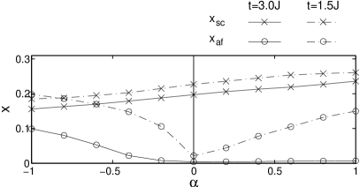
Figure 2: Plot of the doping level $x_{af}$ at which $d$-wave SC order replaces AF order (circles) and of the maximum doping level $x_{sc}$ of the $d$-wave SC dome (crosses) as a function of $t^{\prime}=-2t^{\prime\prime}=-\alpha J$ for both $t=3.0J$ (solid line) and $t=1.5J$ (dash-dot line). Note that $\alpha=1$ and $\alpha=-1$ reproduce the hole doped parameters in (42) and the electron doped parameters in (43) respectively.

The phase diagrams in Fig. 1 show that as we move away from half-filling the AF phase is initially replaced by a state where spins are paired in the $d$-wave singlet channel. This $d$-wave gapped spin liquid state enhances the doped carrier kinetic energy while preserving much of the magnetic exchange energy. Gros (1988) As the doping level increases carrier motion further frustrates the exchange energy and eventually closes the $d$-wave gap. Therefore, the doping evolution of phases is closely connected to the doped carrier dynamics and, below, we explore the microscopic picture that underlies how the hopping parameters $t$, $t^{\prime}$ and $t^{\prime\prime}$ affect the robustness of AF and SC correlations (see the different phase diagrams in Fig. 1 as well as how $x_{af}$ and $x_{sc}$, which stand for the doping level at which $d$-wave SC order replaces AF order and the maximum doping level of the $d$-wave SC dome, change with $t$ and $t^{\prime}=-2t^{\prime\prime}$ in Fig. 2).

The combined effect of the $t$, $t^{\prime}$ and $t^{\prime\prime}$ terms may enhance or deplete the hopping between first, second and third NN sites and, thus, increase or decrease the coupling between doped carriers and specific surrounding spin correlations. The particular case of NN hopping is controlled by $t$ and it frustrates the spin correlations induced by the exchange term in the Hamiltonian. Hence, increasing $t/J$ enfeebles antiferromagnetism and reduces the $d$-wave spin pairing amplitude $\Delta$, as supported by the decrease of both $x_{af}$ and $x_{sc}$ in Fig. 2 when we go from $t=3J$ to $t=1.5J$.

The hopping between second NN sites is controlled both by $t$ and $t^{\prime}$ – if the latter parameter is positive then $t$ and $t^{\prime}$ processes interfere constructively to enhance second NN hopping, while if $t^{\prime}<0$ these processes interfere destructively to deplete second NN hopping. The same argument applies to third NN hopping if we take $t^{\prime\prime}$ instead of $t^{\prime}$ above. Since both second and third NN hopping do not harm the staggered spin configuration of the AF state, increasing either $t^{\prime}$ (as in the ED side) or $t^{\prime\prime}$ (as in the HD side) stabilizes AF order and increases $x_{af}$ (Fig. 2). $t^{\prime}$ in the ED regime is larger than $t^{\prime\prime}$ in the HD regime and, therefore, this effect is more prominent in the former case, leading to the aforementioned asymmetry in the phase diagrams.

Figs. 1 and 2 support that the values of $t^{\prime}$ and $t^{\prime\prime}$ also affect how doped carrier motion couples to $d$-wave SC correlations. To understand this effect note that, in a $d$-wave superconductor, the condensate induces intra-sublattice hopping processes where the amplitude for a hole to hop between second NN sites is negative while the amplitude for a hole to hop between third NN sites is positive. These processes, and thus SC order as well, are frustrated when $t^{\prime}=-2t^{\prime\prime}>0$. A different way to picture the above argument is to note that when $t^{\prime}=-2t^{\prime\prime}>0$ the doped carrier dispersion is gaped at $(\tfrac{\pi}{2},\tfrac{\pi}{2})$, in which case, a vacancy hopping in the presence of local AF correlations frustrates the spinon $d_{x^{2}-y^{2}}$-wave dispersion and weakens superconductivity. Therefore, $x_{sc}$ decreases when $t^{\prime}$ and $t^{\prime\prime}$ vary between the HD and ED regimes (Fig. 2). The same applies to the highest SC T_c, in agreement with experiments and other theoretical approaches. Indeed, band theory calculations together with experimental data support that the maximum T_c for various cuprate families increases with $-t^{\prime}/t$. Pavarini et al. (2001) ARPES results also suggest the correlation between the high energy pseudogap scale, which is controlled by $t^{\prime}$ and $t^{\prime\prime}$, and the maximum T_c. Tanaka et al. (2004) In addition, variational Monte Carlo calculations further substantiate the above role of $t^{\prime}$ in determining the robustness of SC correlations. Shih et al. (2004)

The previous digression on the roles played by $t$, $t^{\prime}$ and $t^{\prime\prime}$ in the interplay between spin and charge degrees of freedom may be of interest to understand the striking differences between as-grown and oxygen reduced electron doped cuprate compounds. The former samples are not SC and display long-range AF order up to $x\approx 0.20$. Mang et al. (2004) After the oxygen reduction process, which removes about $1\%$ of the oxygen atoms in these materials, AF order is destroyed at $x\approx 0.10-0.14$ and, at higher doping values, the samples superconduct. Takagi et al. (1989b); Luke et al. (1990); Fujita et al. (2003) Within the present context, we propose this sharp change follows the alteration of the effective in-plane parameters $t$, $t^{\prime}$ and $t^{\prime\prime}$. Since both $t^{\prime}$ and $t^{\prime\prime}$ depend on the chemical composition outside the copper-oxide layers, Pavarini et al. (2001) if such a composition changes in a way that the magnitude of $t^{\prime}$ and $t^{\prime\prime}$ decreases, the phase-space volume of the AF phase is reduced while SC correlations are enhanced. Alternatively, if the oxygen reduction process acts on the copper-oxide planes in such a manner that $t$ effectively decreases, then $\tfrac{t}{J}\sim\tfrac{U}{t}$ increases, which favors superconductivity over antiferromagnetism. The latter scenario receives support from experimental evidence for the removal of oxygen atoms from the copper-oxide planes under the reduction process in both PCCO Riou et al. (2004) and NCCO. Richard et al. (2004)

V Summary

In this paper we explicitly derive a recently introduced Ribeiro and Wen (2005) formulation of the $tt^{\prime}t^{\prime\prime}J$ model in terms of projected dopon and spin operators instead of projected electron and spin operators. Since dopons describe the carriers doped in the half-filled system, we name it the “doped carrier” formulation of the $tt^{\prime}t^{\prime\prime}J$ model. Close to half-filling the doped carrier density is small and, thus, we circumvent the “no-double-occupancy” constraint. In particular, we propose that the effect of the projection operators $\mathcal{P}$ in the usual formulation of the $tt^{\prime}t^{\prime\prime}J$ model (1) is captured by the interaction between doped carriers and lattice spins in (13). This interaction explicitly accounts for the interplay between local spin correlations and the hole dynamics in doped Mott insulators.

The $tt^{\prime}t^{\prime\prime}J$ model Hamiltonian in the enlarged Hilbert space [Expression (10)] provides a new starting point to deal with doped spin models, which we pursue to develop a new, fully fermionic, MF theory of doped Mott insulators. The resulting “doped carrier” MF theory is constructed to address the low doping and low temperature regime of the $tt^{\prime}t^{\prime\prime}J$ model, and properly accounts for the frustration of NN hopping due to the strong local AF correlations present in such a limit. Since a hole hopping in an antiferromagneticaly correlated spin background induces new local spin correlations that strongly renormalize $t^{\prime}$ and $t^{\prime\prime}$, Ribeiro (2004) in (41) we introduce a phenomenological doping dependent renormalization factor $r(x)$. Specifically, we choose $r(x)$ so that the high energy MF dispersion $\epsilon_{2,\bm{k}}^{-}$ reproduces the evolution of the high energy pseudogap scale at $(0,\pi)$ observed in ARPES experiments. Damascelli et al. (2003); Tanaka et al. (2004) Remarkably, using $t$, $t^{\prime}$ and $t^{\prime\prime}$ motivated by band theory Hybertsen et al. (1990); Pavarini et al. (2001) and with the aforementioned little experimental input the “doped carrier” MF theory leads to a semi-quantitative correct phase diagram for both HD and ED cuprates [Fig. 1(a)]. In particular, in the HD case a large SC dome and extended pseudogap regime are obtained, while superconductivity is much weaker on the ED side where it is partly overtaken by the robust AF phase.

In the low doping limit of the generalized-$tJ$ model it is meaningful, and we believe useful as well, to think of vacancies encircled by local moments. The “doped carrier” approach then provides a framework to address the hole dynamics in the presence of various local spin correlations. In the hereby developed MF theory, an effective multi-band description captures the effect of two different local correlations, namely staggered moment and $d$-wave singlet bond correlations: the vacancy in the one-dopon state is encircled by staggered local moments which inhibit NN hopping; upon spinon-dopon mixing the vacancy changes the surrounding spin background and gains kinetic energy, which is the driving force for the $d$-wave SC state at low doping. The above two-band description receives support from more rigorous calculations on the two-dimensional $tJ$ and Hubbard models, Moreo et al. (1995); Preuss et al. (1995); Dorneich et al. (2000); Gröber et al. (2000); Ribeiro (2004); Kyung et al. (2006) and is consistent with the various spectral features observed by ARPES experiments. Ronning et al. (2003); Kohsaka et al. (2003); Yoshida et al. (2003); Shen et al. (2004) We remark that in the present approach superconductivity arises due to the change imposed on spin correlations by the motion of doped carriers. This process is captured by the spinon-dopon mixing, which can be viewed as a new mechanism for superconductivity. We believe this mechanism to be relevant for the experimentally obtained low values of $J/t$. In the large $J/t$ regime a distinct mechanism, namely the minimization of the number of missing AF links, may lead doped carriers to form local pairs, as proposed by the “antiferromagnetic-van Hove model”. Dagotto et al. (1995)

Since the “doped carrier” approach addresses the interplay between the doped carrier dynamics and different background correlations, we can discuss how the strength of the latter depends on the hopping parameters. Interestingly, we find that short-range AF correlations can enhance or deplete $d$-wave SC correlations depending on the sign of $t^{\prime}$ and $t^{\prime\prime}$. Specifically, if these hopping parameters favor a gap in the single hole $tt^{\prime}t^{\prime\prime}J$ model dispersion at $(\tfrac{\pi}{2},\tfrac{\pi}{2})$, as in the ED regime, the vacancies when in the presence of local AF configurations frustrate the $d$-wave SC gap and, thus, superconductivity as well. The opposite effect occurs if, instead, $t^{\prime}$ and $t^{\prime\prime}$ induce a gap at $(0,\pi)$ in the single hole $tt^{\prime}t^{\prime\prime}J$ model dispersion. Hence, the interplay between short-range AF and $d$-wave SC correlations provides a microscopic rational for the role of $t^{\prime}$ and $t^{\prime\prime}$ in strengthening superconductivity as expected by experiments and other theoretical approaches. Pavarini et al. (2001); Tanaka et al. (2004); Shih et al. (2004) In this context, note that the “doped carrier” MF theory not only accounts for the hole/electron doped asymmetry but also offers possible scenarios for the difference between phase diagrams of as-grown and oxygen reduced electron doped samples. Mang et al. (2004); Takagi et al. (1989b); Luke et al. (1990); Fujita et al. (2003)

The “doped carrier” formulation provides a MF theory to describe superconductors with strong local AF correlations due to a proximate Mott insulating state. The signature of such correlations is explicit in a variety of cuprate experimental data that deviates from the pure BCS behavior. In particular, Refs. Ribeiro and Wen, 2005, , 2001 show that several non-trivial features of the electron spectral function and of the tunneling conductance spectrum of cuprates are reproduced by the herein presented MF approach.

Appendix A Relation to slave-boson approach

In the present paper a new formulation of the $tt^{\prime}t^{\prime\prime}J$ model is used as a starting point to develop a new MF theory of doped Mott insulators. This “doped carrier” MF theory, which to the authors’ best knowledge differs from other MF theories in the literature, bears some relations to the slave-boson MF approach to the same model. SLA Both approximations recur to the fermionic representation of spin operators and, thus, in the undoped limit both MF approaches are equivalent. However, these MF theories deal with doped carriers in distinct manners since they introduce different operators to account for charged degrees of freedom in doped systems – the slave-boson formulation introduces the spinless charged bosonic holon operator $h_{i}^{\dagger}=[h_{i,1}^{\dagger}h_{i,2}^{\dagger}]$ while the “doped carrier” formulation introduces the spin-1/2 charged fermionic dopon operator $d_{i}^{\dagger}$. In this appendix we clarify the relation between holon and dopon operators and, thus, the relation between the extensively used slave-boson approach and the new “doped carrier” formalism.

Within slave-boson theory, the projected electron operators, which are the building blocks of all other physical operators, can be written in terms of holons and spinons as

$$\mathcal{P}c_{i,\uparrow}^{\dagger}\mathcal{P} =\frac{1}{\sqrt{2}}\left(h_{i,1}f_{i,\uparrow}^{\dagger}+h_{i,2}f_{i,\downarrow}\right)$$

$$\mathcal{P}c_{i,\downarrow}^{\dagger}\mathcal{P} =\frac{1}{\sqrt{2}}\left(h_{i,1}f_{i,\downarrow}^{\dagger}-h_{i,2}f_{i,\uparrow}\right)$$ (47)

as long as we constrain ourselves to the physical Hilbert space defined by $(\psi_{i}^{\dagger}\bm{\sigma}\psi_{i}+h_{i}^{\dagger}\bm{\sigma}h_{i})=0$. Wen and Lee (1996); Lee et al. (1998) This formulation introduces an $SU(2)$ gauge structure since physical operators are invariant under the local transformation $\psi_{i}\rightarrow W_{i}\psi_{i}$ and $h_{i}\rightarrow W_{i}h_{i}$, where $W_{i}$ is any $SU(2)$ matrix. Hence, both spinons and holons carry an $SU(2)$ gauge charge in addition to the physical spin and electric charge quantum numbers.

Interestingly, in the “doped carrier” formalism dopons and spinons can form singlet pairs, as captured by the operators $\widehat{B}_{i,j}$ introduced in Sec. III.2. These are electrically charged spinless bosonic fields which also carry the above $SU(2)$ gauge charge and, therefore, they have the same quantum numbers as holon operators in the slave-boson framework. To make the relation between holons and spinon-dopon pairs explicit it is convenient to rewrite the projected electron operators in terms of dopons and spinons. We use $\widetilde{S}_{i}^{z}=\tfrac{1}{2}\left(f_{i,\uparrow}^{\dagger}f_{i,\uparrow}-f_{i,\downarrow}^{\dagger}f_{i,\downarrow}\right)$, $\widetilde{S}_{i}^{+}=f_{i,\uparrow}^{\dagger}f_{i,\downarrow}$ and $\widetilde{S}_{i}^{-}=f_{i,\downarrow}^{\dagger}f_{i,\uparrow}$ to express the operators in (9) as

$$\mathcal{P}c_{i,\uparrow}^{\dagger}\mathcal{P} =\frac{1}{\sqrt{2}}f_{i,\uparrow}^{\dagger}\widetilde{\mathcal{P}}\left(f_{i,\uparrow}d_{i,\downarrow}-f_{i,\downarrow}d_{i,\uparrow}\right)\widetilde{\mathcal{P}}$$

$$\mathcal{P}c_{i,\downarrow}^{\dagger}\mathcal{P} =\frac{1}{\sqrt{2}}f_{i,\downarrow}^{\dagger}\widetilde{\mathcal{P}}\left(f_{i,\uparrow}d_{i,\downarrow}-f_{i,\downarrow}d_{i,\uparrow}\right)\widetilde{\mathcal{P}}$$ (48)

Since the above equality only holds for $f_{i}^{\dagger}f_{i}=1$ it can be recast as

$$\mathcal{P}c_{i,\uparrow}^{\dagger}\mathcal{P} =\frac{1}{\sqrt{2}}f_{i,\downarrow}\widetilde{\mathcal{P}}\left(f_{i,\uparrow}^{\dagger}d_{i,\uparrow}+f_{i,\downarrow}^{\dagger}d_{i,\downarrow}\right)\widetilde{\mathcal{P}}$$

$$\mathcal{P}c_{i,\downarrow}^{\dagger}\mathcal{P} =-\frac{1}{\sqrt{2}}f_{i,\uparrow}\widetilde{\mathcal{P}}\left(f_{i,\uparrow}^{\dagger}d_{i,\uparrow}+f_{i,\downarrow}^{\dagger}d_{i,\downarrow}\right)\widetilde{\mathcal{P}}$$ (49)

Using the slave-boson formulation language, in the physical Hilbert space there can be at most one holon per site. Say it happens to be a $h_{i,1}$ holon. Then, the projected electron operators in (47) resemble those in (48) with the $h_{i,1}$ holon replaced by the spinon-dopon pair $\left(f_{i,\uparrow}d_{i,\downarrow}-f_{i,\downarrow}d_{i,\uparrow}\right)$. If, instead, there exists a $h_{i,2}$ holon on site $i$, the projected electron operators in (47) resemble those in (49) with the $h_{i,2}$ holon replaced by the spinon-dopon pair $\left(f_{i,\uparrow}^{\dagger}d_{i,\uparrow}+f_{i,\downarrow}^{\dagger}d_{i,\downarrow}\right)$. In this sense, the $h_{i,1}$ and $h_{i,2}$ holon operators are related to specific singlet pairs of spinons and dopons.

The above correspondence between holons and spinon-dopon pairs can be used to compare MF phases in the slave-boson and “doped carrier” approaches. Specifically, for a given spinon state, the physical symmetries of a phase described by a certain pattern of holon condensation $\langle h_{i}^{\dagger}\rangle=[\langle h_{i,1}^{\dagger}\rangle\langle h_{i,2}^{\dagger}\rangle]$ in the slave-boson formulation are the same as those of a state where spinon-dopon pairing in the “doped carrier” formulation yields

$$B_{i0}=\left[\begin{array}[]{cc}-\langle h_{i,2}\rangle&\langle h_{i,1}\rangle\\ \langle h_{i,1}^{\dagger}\rangle&\langle h_{i,2}^{\dagger}\rangle\end{array}\right]$$ (50)

This result shows that holon condensation in the slave-boson formalism leads to the same phases as the spinon-dopon pairing transition observed in the “doped carrier” approach. In particular, in the presence of $d$-wave paired spinons described by ansatz (20), the $d$-wave SC state obtained upon the condensation of holons $\langle h_{i}^{\dagger}\rangle=[0\ h_{0}]$ is the same as the one that occurs in the presence of the spinon-dopon pairing described in (29).

To understand the connection between holons and spinon-dopon pairs it is useful to consider the local picture of these objects. The dopon is an entity which carries charge and spin and is formed by the vacancy plus a neighboring spin. More precisely, the dopon spin is carried by the staggered local moments that surround the vacancy in the one-dopon state. Since these local moments frustrate doped carrier hopping the spin state encircling the vacancy in the one-dopon state is modified to optimize the doped carrier kinetic energy. In the “doped carrier” MF theory this interaction between doped carriers and the surrounding spins is captured by the $\sim d^{\dagger}ff^{\dagger}d$ term in (22) which can be recast as $\sim bf^{\dagger}d$. This term drives the decay of the dopon into a spinless spinon-dopon pair and a chargeless spinon. Physically, this process means that the spin background forms a singlet with the dopon spin thus altering the spin configuration around the vacancy. The vacancy is then encircled by a local spin singlet configuration, which corresponds to the local picture of a holon. The doped carrier spin-1/2 is absorbed by the spin background in the form of a spinon excitation.

The above picture suggests that the holon is a composite object and that the “doped carrier” approach captures its internal structure. Such an internal structure should then be apparent in the electronic spectral properties. In Ref. Ribeiro and Wen, these properties are discussed at length and the holon internal structure is argued to be reflected in the momentum space anisotropy (also known as the nodal-antinodal dichotomy Zhou et al. (2004)) of the electron spectral function.

Appendix B Paramagnetic mean-field self-consistency equations

Below we write the set of self-consistent conditions for the paramagnetic MF Hamiltonian (36) which are determined by the saddle point equations

$$\frac{\partial F}{\partial\chi}=\frac{\partial F}{\partial\Delta}=\frac{\partial F}{\partial b_{0}}=\frac{\partial F}{\partial b_{1}}=\frac{\partial F}{\partial\mu_{d}}=\frac{\partial F}{\partial a_{0}}=0$$ (51)

where $F$ is the MF free-energy of the fermionic system described by (36), namely

$$\frac{F}{N} =\frac{3\tilde{J}}{4}\left(\chi^{2}+\Delta^{2}\right)-2b_{0}b_{1}-\mu_{d}(1-x)-$$

$$\quad-\frac{T}{N}\sum_{\bm{k}}\ln\left[1+\cosh\left(\frac{\epsilon_{1,\bm{k}}^{+}}{T}\right)\right]\left[1+\cosh\left(\frac{\epsilon_{2,\bm{k}}^{+}}{T}\right)\right]$$ (52)

The resulting self-consistent equations for the mean-fields $\chi$, $\Delta$, $b_{0}$ and $b_{1}$, as well as the doping concentration and $SU(2)$ projection constraints, are:

$$\chi=-\frac{1}{4N}\sum_{\bm{k}}\left(\cos k_{x}+\cos k_{y}\right)\left\{\alpha_{\bm{k}}^{z}A_{\bm{k}}-\frac{2\gamma_{\bm{k}}\beta_{\bm{k}}^{2}+\alpha_{\bm{k}}^{z}\left[2\beta_{\bm{k}}^{2}+\left(\alpha_{\bm{k}}^{x}\right)^{2}+\left(\alpha_{\bm{k}}^{z}\right)^{2}-\gamma_{\bm{k}}^{2}\right]}{2\sqrt{\delta_{\bm{k}}}}B_{\bm{k}}\right\}$$ (53)

$$\Delta=-\frac{1}{4N}\sum_{\bm{k}}\alpha_{\bm{k}}^{x}\left(\cos k_{x}-\cos k_{y}\right)\left\{A_{\bm{k}}-\frac{2\beta_{\bm{k}}^{2}+\left(\alpha_{\bm{k}}^{x}\right)^{2}+\left(\alpha_{\bm{k}}^{z}\right)^{2}-\gamma_{\bm{k}}^{2}}{2\sqrt{\delta_{\bm{k}}}}B_{\bm{k}}\right\}$$ (54)

$$b_{1}=-\frac{3}{16N}\sum_{\bm{k}}\beta_{\bm{k}} \left[t_{1}\left(\cos k_{x}+\cos k_{y}\right)+2t_{2}\cos k_{x}\cos k_{y}+t_{3}\left(\cos 2k_{x}+\cos 2k_{y}\right)\right]\times$$

$$\times\left\{A_{\bm{k}}-\frac{\left(\gamma_{\bm{k}}+\alpha_{\bm{k}}^{z}\right)^{2}+\left(\alpha_{\bm{k}}^{x}\right)^{2}}{2\sqrt{\delta_{\bm{k}}}}B_{\bm{k}}\right\}$$ (55)

$$b_{0}=-\frac{1}{2N}\sum_{\bm{k}}\beta_{\bm{k}}\left\{A_{\bm{k}}-\frac{\left(\gamma_{\bm{k}}+\alpha_{\bm{k}}^{z}\right)^{2}+\left(\alpha_{\bm{k}}^{x}\right)^{2}}{2\sqrt{\delta_{\bm{k}}}}B_{\bm{k}}\right\}$$ (56)

$$x=1-\frac{1}{2N}\sum_{\bm{k}}\left\{\gamma_{\bm{k}}A_{\bm{k}}-\frac{2\alpha_{\bm{k}}^{z}\beta_{\bm{k}}^{2}+\gamma_{\bm{k}}\left[2\beta_{\bm{k}}^{2}+\gamma_{\bm{k}}^{2}-\left(\alpha_{\bm{k}}^{x}\right)^{2}-\left(\alpha_{\bm{k}}^{z}\right)^{2}\right]}{2\sqrt{\delta_{\bm{k}}}}B_{\bm{k}}\right\}$$ (57)

$$0=\frac{1}{2N}\sum_{\bm{k}}\left\{\alpha_{\bm{k}}^{z}A_{\bm{k}}-\frac{2\gamma_{\bm{k}}\beta_{\bm{k}}^{2}+\alpha_{\bm{k}}^{z}\left[2\beta_{\bm{k}}^{2}+\left(\alpha_{\bm{k}}^{x}\right)^{2}+\left(\alpha_{\bm{k}}^{z}\right)^{2}-\gamma_{\bm{k}}^{2}\right]}{2\sqrt{\delta_{\bm{k}}}}B_{\bm{k}}\right\}$$ (58)

where we introduce

$$A_{\bm{k}}=\frac{\sinh\left(\frac{\epsilon_{1,\bm{k}}^{+}}{T}\right)}{\epsilon_{1,\bm{k}}^{+}\left[1+\cosh\left(\frac{\epsilon_{1,\bm{k}}^{+}}{T}\right)\right]}+\frac{\sinh\left(\frac{\epsilon_{2,\bm{k}}^{+}}{T}\right)}{\epsilon_{2,\bm{k}}^{+}\left[1+\cosh\left(\frac{\epsilon_{2,\bm{k}}^{+}}{T}\right)\right]}$$ (59)

and

$$B_{\bm{k}}=\frac{\sinh\left(\frac{\epsilon_{1,\bm{k}}^{+}}{T}\right)}{\epsilon_{1,\bm{k}}^{+}\left[1+\cosh\left(\frac{\epsilon_{1,\bm{k}}^{+}}{T}\right)\right]}-\frac{\sinh\left(\frac{\epsilon_{2,\bm{k}}^{+}}{T}\right)}{\epsilon_{2,\bm{k}}^{+}\left[1+\cosh\left(\frac{\epsilon_{2,\bm{k}}^{+}}{T}\right)\right]}$$ (60)

The remaining notation is defined in (37) and (39).

Appendix C Antiferromagnetic mean-field self-consitency equations

In Sec. III.6 we extend the “doped carrier” MF theory to include the staggered magnetization decoupling channel and obtain the MF Hamiltonian (46). In this paper we do not consider states with coexisting AF and SC order and, in what follows, we set $b_{0}$ and $b_{1}$ to zero in (46). Since in this case spinons and dopons do not mix we can define two spinon and two dopon bands, namely

$$\epsilon_{s,\bm{k}}^{\pm}=\pm\sqrt{\left(\alpha_{\bm{k}}^{x}\right)^{2}+\left(\alpha_{\bm{k}}^{z}\right)^{2}+\nu_{\bm{k}}^{2}}$$

$$\epsilon_{d,\bm{k}}^{\pm}=\left(1\mp 2|m|\right)\gamma_{\bm{k}}-\mu_{d}$$ (61)

where $\nu_{\bm{k}}=-2\left(J^{*}m-n\right)$. In the absence of spinon-dopon hybridization $a_{0}=0$ and $\alpha_{\bm{k}}^{z}=-\left(\frac{3\tilde{J}}{4}\chi-\frac{t_{1}x}{2}\right)\left(\cos k_{x}+\cos k_{y}\right)$.

The resulting MF free-energy is

$$\frac{F}{N} =\frac{3\tilde{J}}{4}\left(\chi^{2}+\eta^{2}\right)+2J^{*}m^{2}-4mn-\mu_{d}(1-x)-$$

$$\quad-\frac{T}{N}\sum_{\bm{k}}\left\{\ln\left[\cosh\left(\frac{\gamma_{\bm{k}}-\mu_{d}}{T}\right)+\cosh\left(\frac{2m\gamma_{\bm{k}}}{T}\right)\right]+\right.$$

$$\quad\quad\quad\quad\quad\quad\left.+\ln\left[1+\cosh\left(\frac{\epsilon_{s,\bm{k}}^{+}}{T}\right)\right]\right\}$$ (62)

and the self-consistency equations

$$\frac{\partial F}{\partial\chi}=\frac{\partial F}{\partial\Delta}=\frac{\partial F}{\partial m}=\frac{\partial F}{\partial n}=\frac{\partial F}{\partial\mu_{d}}=0$$ (63)

reduce to

$$\chi=-\frac{1}{2N}\sum_{\bm{k}}\frac{\alpha_{\bm{k}}^{z}\left(\cos k_{x}+\cos k_{y}\right)}{\epsilon_{s,\bm{k}}^{+}}\frac{\sinh\left(\frac{\epsilon_{s,\bm{k}}^{+}}{T}\right)}{1+\cosh\left(\frac{\epsilon_{s,\bm{k}}^{+}}{T}\right)}$$ (64)

$$\Delta=-\frac{1}{2N}\sum_{\bm{k}}\frac{\alpha_{\bm{k}}^{x}\left(\cos k_{x}-\cos k_{y}\right)}{\epsilon_{s,\bm{k}}^{+}}\frac{\sinh\left(\frac{\epsilon_{s,\bm{k}}^{+}}{T}\right)}{1+\cosh\left(\frac{\epsilon_{s,\bm{k}}^{+}}{T}\right)}$$ (65)

$$m=\frac{1}{N}\sum_{\bm{k}}\frac{J^{*}m-n}{\epsilon_{s,\bm{k}}^{+}}\frac{\sinh\left(\frac{\epsilon_{s,\bm{k}}^{+}}{T}\right)}{1+\cosh\left(\frac{\epsilon_{s,\bm{k}}^{+}}{T}\right)}$$ (66)

$$n=-\frac{1}{2N}\sum_{\bm{k}}\frac{\gamma_{\bm{k}}\sinh\left(\frac{2m\gamma_{\bm{k}}}{T}\right)}{\cosh\left(\frac{\gamma_{\bm{k}}-\mu_{d}}{T}\right)+\cosh\left(\frac{2m\gamma_{\bm{k}}}{T}\right)}$$ (67)

$$x=1-\frac{1}{N}\sum_{\bm{k}}\frac{\sinh\left(\frac{\gamma_{\bm{k}}-\mu_{d}}{T}\right)}{\cosh\left(\frac{\gamma_{\bm{k}}-\mu_{d}}{T}\right)+\cosh\left(\frac{2m\gamma_{\bm{k}}}{T}\right)}$$ (68)

References

- Anderson (1987) P. W. Anderson, Science 235, 1196 (1987).
- Kastner et al. (1998) M. A. Kastner, R. J. Birgeneau, G. Shirane, and Y. Endoh, Rev. Mod. Phys. 70, 897 (1998).
- Lee et al. (2004) P. A. Lee, N. Nagaosa, and X.-G. Wen, cond-mat/0410445 (2004).
- Dagotto (1994) E. Dagotto, Rev. Mod. Phys. 66, 763 (1994).
- Pavarini et al. (2001) E. Pavarini, I. Dasgupta, T. Saha-Dasgupta, O. Jepsen, and O. K. Andersen, Phys. Rev. Lett. 87, 047003 (2001).
- Tohyama and Maekawa (2000) T. Tohyama and S. Maekawa, Supercond. Sci. Technol. 13, R17 (2000).
- Tohyama (2004) T. Tohyama, Phys. Rev. B 70, 174517 (2004).
- Ribeiro (2004) T. C. Ribeiro, cond-mat/0409002 (2004).
- Moreo et al. (1995) A. Moreo, S. Haas, A. W. Sandvik, and E. Dagotto, Phys. Rev. B 51, R12045 (1995).
- Kim et al. (1998) C. Kim, P. J. White, Z.-X. Shen, T. Tohyama, Y. Shibata, S. Maekawa, B. O. Wells, Y. J. Kim, R. J. Birgeneau, and M. A. Kastner, Phys. Rev. Lett. 80, 4245 (1998).
- Tohyama and Maekawa (1994) T. Tohyama and S. Maekawa, Phys. Rev. B 49, 3596 (1994).
- Gooding et al. (1994) R. J. Gooding, K. J. E. Vos, and P. W. Leung, Phys. Rev. B 50, 12866 (1994).
- Nishimoto et al. (1998) S. Nishimoto, Y. Ohta, and R. Eder, Phys. Rev. B 57, R5590 (1998).
- Schmitt-Rink et al. (1988) S. Schmitt-Rink, C. M. Varma, and A. E. Ruckenstein, Phys. Rev. Lett. 60, 2793 (1988).
- Xiang and Wheatley (1996) T. Xiang and J. M. Wheatley, Phys. Rev. B 54, R12653 (1996).
- Belinicher et al. (1996) V. I. Belinicher, A. L. Chernyshev, and V. A. Shubin, Phys. Rev. B 54, 14914 (1996).
- Martinez and Horsch (1991) G. Martinez and P. Horsch, Phys. Rev. B 44, 317 (1991).
- Liu and Manousakis (1992) Z. Liu and E. Manousakis, Phys. Rev. B 45, 2425 (1992).
- Nazarenko et al. (1995) A. Nazarenko, K. J. E. Vos, S. Haas, E. Dagotto, and R. J. Gooding, Phys. Rev. B 51, 8676 (1995).
- Kyung et al. (2006) B. Kyung, S. S. Kancharla, D. Sénéchal, A.-M. S. Tremblay, M. Civelli, and G. Kotliar, Phys. Rev. B 73, 165114 (2006).
- Preuss et al. (1995) R. Preuss, W. Hanke, and W. von der Linden, Phys. Rev. Lett. 75, 1344 (1995).
- Dorneich et al. (2000) A. Dorneich, M. G. Zacher, C. Gröber, and R. Eder, Phys. Rev. B 61, 12816 (2000).
- Gröber et al. (2000) C. Gröber, R. Eder, and W. Hanke, Phys. Rev. B 62, 4336 (2000).
- Duffy and Moreo (1995) D. Duffy and A. Moreo, Phys. Rev. B 51, 11882 (1995).
- Dagotto et al. (1994) E. Dagotto, A. Nazarenko, and M. Boninsegni, Phys. Rev. Lett. 73, 728 (1994).
- Dagotto et al. (1995) E. Dagotto, A. Nazarenko, and A. Moreo, Phys. Rev. Lett. 74, 310 (1995).
- Shih et al. (2004) C. T. Shih, T. K. Lee, R. Eder, C.-Y. Mou, and Y. C. Chen, Phys. Rev. Lett. 92, 227002 (2004).
- Gros (1988) C. Gros, Phys. Rev. B 38, 931 (1988).
- Sorella et al. (2002) S. Sorella, G. B. Martins, F. Becca, C. Gazza, L. Capriotti, A. Parola, and E. Dagotto, Phys. Rev. Lett. 88, 117002 (2002).
- Paramekanti et al. (2004) A. Paramekanti, M. Randeria, and N. Trivedi, Phys. Rev. B 70, 054504 (2004).
- Zhang et al. (1988) F. C. Zhang, C. Gros, T. M. Rice, and H. Shiba, Supercond. Sci. Technol. 1, 36 (1988).
- Gutzwiller (1963) M. C. Gutzwiller, Phys. Rev. Lett. 10, 159 (1963).
- Wen and Lee (1996) X.-G. Wen and P. A. Lee, Phys. Rev. Lett. 76, 503 (1996).
- Lee et al. (1998) P. A. Lee, N. Nagaosa, T.-K. Ng, and X.-G. Wen, Phys. Rev. B 57, 6003 (1998).
- Barnes (1976) S. E. Barnes, J. Phys. F 6, 1375 (1976).
- Coleman (1984) P. Coleman, Phys. Rev. B 29, 3035 (1984).
- G.Baskaran et al. (1987) G.Baskaran, Z. Zou, and P. W. Anderson, Solid State Commun. 63, 973 (1987).
- Baskaran and Anderson (1988) G. Baskaran and P. W. Anderson, Phys. Rev. B 37, R580 (1988).
- Affleck et al. (1988) I. Affleck, Z. Zou, T. Hsu, and P. W. Anderson, Phys. Rev. B 38, 745 (1988).
- Lee and Nagaosa (1992) P. A. Lee and N. Nagaosa, Phys. Rev. B 46, 5621 (1992).
- Kotliar and Liu (1988) G. Kotliar and J. Liu, Phys. Rev. B 38, R5142 (1988).
- (42) Right at half-filling .
- Ribeiro and Wen (2005) T. C. Ribeiro and X.-G. Wen, Phys. Rev. Lett. 95, 057001 (2005).
- (44) Here we assume that the hole doped into the spin system does not create a ferromagnetic polaron. This is believed to be the case unless is an order of magnitude smaller than observed in material compounds like the cuprates White and Affleck (2001).
- (45) Band insulators have two valence electrons per site, hence, a hole on a certain site leaves a charge and spin in this same site.
- Manousakis (1991) E. Manousakis, Rev. Mod. Phys. 63, 1 (1991).
- Damascelli et al. (2003) A. Damascelli, Z.-X. Shen, and Z. Hussain, Rev. Mod. Phys. 75, 473 (2003).
- Ronning et al. (2003) F. Ronning, T. Sasagawa, Y. Kohsaka, K. M. Shen, A. Damascelli, C. Kim, T. Yoshida, N. P. Armitage, D. H. Lu, D. L. Feng, et al., Phys. Rev. B 67, 165101 (2003).
- Kohsaka et al. (2003) Y. Kohsaka, T. Sasagawa, F. Ronning, T. Yoshida, C. Kim, T. Hanaguri, M. Azuma, M. Takano, Z.-X. Shen, and H. Takagi, J. Phys. Soc. Jpn. 72, 1018 (2003).
- Shen et al. (2004) K. M. Shen, F. Ronning, D. H. Lu, W. S. Lee, N. J. C. Ingle, W. Meevasana, F. Baumberger, A. Damascelli, N. P. Armitage, L. L. Miller, et al., Phys. Rev. Lett. 93, 267002 (2004).
- Yoshida et al. (2003) T. Yoshida, X. J. Zhou, T. Sasagawa, W. L. Yang, P. V. Bogdanov, A. Lanzara, Z. Hussain, T. Mizokawa, A. Fujimori, H. Eisaki, et al., Phys. Rev. Lett. 91, 027001 (2003).
- (52) T. C. Ribeiro and X.-G. Wen, in preparation.
- Ribeiro and Wen (2001) T. C. Ribeiro and X.-G. Wen, cond-mat/0511031 (2001).
- Norman et al. (1998) M. R. Norman, H. Ding, M. Randeria, J. C. Campuzano, T. Yokoya, T. Takeuchi, T. Takahashi, T. Mochiku, K. Kadowaki, P. Guptasarma, et al., Nature 392, 157 (1998).
- (55) In the electron doped regime the states , and rather represent a spin-up hole, a spin-down hole and a site with no holes respectively. Therefore, in that case, the operator in (9) is a hole creation operator.
- (56) In Sec. III we introduce the fermionic representation of the lattice spin operators , where is the spinon creation spinor operator, which is valid upon the enforcement of the constraint. In such a representation the operator in (9) reduces to . This expression, which holds as long as the local constraint is enforced, can be modified so that it explicitly vanishes in case , specifically (the overall is missed in the similar expression presented in Ref. Ribeiro and Wen, 2005).
- Abrikosov (1965) A. Abrikosov, Physics 2, 5 (1965).
- Wen (2002) X.-G. Wen, Phys. Rev. B 65, 165113 (2002).
- Kane et al. (1989) C. L. Kane, P. A. Lee, and N. Read, Phys. Rev. B 39, 6880 (1989).
- (60) The prefactor in (24) differs from the one in the corresponding expression in Ref. Ribeiro and Wen, 2005 by a factor of .
- Ribeiro and Wen (2003) T. C. Ribeiro and X.-G. Wen, Phys. Rev. B 68, 024501 (2003).
- Rantner and Wen (2002) W. Rantner and X.-G. Wen, Phys. Rev. B 66, 144501 (2002).
- Wells et al. (1995) B. O. Wells, Z.-X. Shen, A. Matsuura, D. M. King, M. A. Kastner, M. Greven, and R. J. Birgeneau, Phys. Rev. Lett. 74, 964 (1995).
- Tohyama et al. (2000) T. Tohyama, Y. Shibata, S. Maekawa, Z.-X. Shen, N. Nagaosa, and L. L. Miller, J. Phys. Soc. Jpn. 69, 9 (2000).
- Tanaka et al. (2004) K. Tanaka, T. Yoshida, A. Fujimori, D. H. Lu, Z.-X. Shen, X.-J. Zhou, H. Eisaki, Z. Hussain, S. Uchida, Y. Aiura, et al., Phys. Rev. B 70, 092503 (2004).
- Hybertsen et al. (1990) M. S. Hybertsen, E. B. Stechel, M. Schluter, and D. R. Jennison, Phys. Rev. B 41, 11068 (1990).
- Sulewski et al. (1990) P. E. Sulewski, P. A. Fleury, K. B. Lyons, S.-W. Cheong, and Z. Fisk, Phys. Rev. B 41, 225 (1990).
- Coldea et al. (2001) R. Coldea, S. M. Hayden, G. Aeppli, T. G. Perring, C. D. Frost, T. E. Mason, S.-W. Cheong, and Z. Fisk, Phys. Rev. Lett. 86, 5377 (2001).
- Takagi et al. (1989a) H. Takagi, T. Ido, S. Ishibashi, M. Uota, S. Uchida, and Y. Tokura, Phys. Rev. B 40, 2254 (1989a).
- Luke et al. (1990) G. M. Luke, L. P. Le, B. J. Sternlieb, Y. J. Uemura, J. H. Brewer, R. Kadono, R. F. Kiefl, S. R. Kreitzman, T. M. Riseman, C. E. Stronach, et al., Phys. Rev. B 42, 7981 (1990).
- Fujita et al. (2003) M. Fujita, T. Kubo, S. Kuroshima, T. Uefuji, K. Kawashima, K. Yamada, I. Watanabe, and K. Nagamine, Phys. Rev. B 67, 014514 (2003).
- Brinckmann and Lee (2002) J. Brinckmann and P. A. Lee, Phys. Rev. B 65, 014502 (2002).
- Sandvik (1997) A. W. Sandvik, Phys. Rev. B 56, 11678 (1997).
- (74) The procedure to determine differs from the one used in Ref. Ribeiro and Wen, 2005 and so does the value of itself. Note that, here, follows from fitting numerical data at half-filling.
- (75) Here we only consider the temperture range displayed in the MF phase diagrams in Ref. Ribeiro and Wen, 2005, in which case we always find that . Only at higher temperatures does vanish and, thus, do the lattice spins decouple from each other at MF level.
- (76) Similar phases also appear in the slave-boson MF phase diagram Wen and Lee (1996) since and arise in both approaches upon the introduction of the fermionic spin representation and given that the spinon-dopon pairing transition which leads to non-zero and is analogous to the holon condensation transition in the slave-boson framework (we further elaborate on this topic in Appendix A).
- Curro et al. (1997) N. J. Curro, T. Imai, C. P. Slichter, and B. Dabrowski, Phys. Rev. B 56, 877 (1997).
- Xu et al. (2000) Z. A. Xu, N. P. Ong, Y. Wang, T. Kakeshita, and S. Uchida, Nature 406, 486 (2000).
- Ong et al. (2004) N. P. Ong, Y. Wang, S. Ono, Y. Ando, and S. Uchida, Annalen der Physik 13, 9 (2004).
- Ussishkin et al. (2002) I. Ussishkin, S. L. Sondhi, and D. A. Huse, Phys. Rev. Lett. 89, 287001 (2002).
- Ussishkin and Sondhi (2004) I. Ussishkin and S. L. Sondhi, Int. J. Mod. Phys. B 18, 3315 (2004).
- Wang et al. (2005) Y. Wang, L. Li, M. J. Naughton, G. D. Gu, S. Uchida, and N. P. Ong, Phys. Rev. Lett. 95, 247002 (2005).
- Ioffe and Larkin (1989) L. B. Ioffe and A. I. Larkin, Phys. Rev. B 39, 8988 (1989).
- (84) The spinon-dopon pairing transition is driven by the kinetic energy gain that results from overcoming the frustration due to the perfect Néel configuration of spins around the vacancy in the one-dopon state [Expression (25)] which, in the above described MF theory, is assumed to be temperature independent. Since increasing temperature reduces the magnitude of the staggered moments around the vacancy, the stability of spinon-dopon mixing at high temperatures is overestimated. Hence, the large phase-space volume taken by the Nernst regime in Fig. 1(a), which extends throughout most of the pseudogap region, should be reduced upon calculating (25) self-consistently. Such a change could shrink the Nernst region for the parameter regime that concerns hole doped cuprates down to the smaller size observed by experiments Ong et al. (2004).
- Balci et al. (2003) H. Balci, C. P. Hill, M. M. Qazilbash, and R. L. Greene, Phys. Rev. B 68, 054520 (2003).
- Mang et al. (2004) P. K. Mang, O. P. Vajk, A. Arvanitaki, J. W. Lynn, and M. Greven, Phys. Rev. Lett. 93, 027002 (2004).
- Takagi et al. (1989b) H. Takagi, S. Uchida, and Y. Tokura, Phys. Rev. Lett. 62, 1197 (1989b).
- Riou et al. (2004) G. Riou, P. Richard, S. Jandl, M. Poirier, P. Fournier, V. Nekvasil, S. N. Barilo, and L. A. Kurnevich, Phys. Rev. B 69, 024511 (2004).
- Richard et al. (2004) P. Richard, G. Riou, I. Hetel, S. Jandl, M. Poirier, and P. Fournier, Phys. Rev. B 70, 064513 (2004).
- (90) The slave-boson formulation and its application to the model have been extensively studied in the literature and we refer the reader to Refs. Barnes, 1976; Coleman, 1984; G.Baskaran et al., 1987; Baskaran and Anderson, 1988; Affleck et al., 1988; Lee and Nagaosa, 1992; Wen and Lee, 1996; Lee et al., 1998, 2004 for additional information.
- Zhou et al. (2004) X. J. Zhou, T. Yoshida, D.-H. Lee, W. L. Yang, V. Brouet, F. Zhou, W. X. Ti, J. W. Xiong, Z. X. Zhao, T. Sasagawa, et al., Phys. Rev. Lett. 92, 187001 (2004).
- White and Affleck (2001) S. R. White and I. Affleck, Phys. Rev. B 64, 024411 (2001).