Nuclear wave function interference in single-molecule electron transport

Abstract

It is demonstrated that non-equilibrium vibrational effects are enhanced in molecular devices for which the effective potential for vibrations is sensitive to the charge state of the device. We calculate the electron tunneling current through a molecule accounting for the two simplest qualitative effects of the charging on the nuclear potential for vibrational motion: a shift (change in the equilibrium position) and a distortion (change in the vibrational frequency). The distortion has two important effects: firstly, it breaks the symmetry between the excitation spectra of the two charge states. This gives rise to new transport effects which map out changes in the current-induced non-equilibrium vibrational distribution with increasing bias voltage. Secondly, the distortion modifies the Franck-Condon factors for electron tunneling. Together with the spectral asymmetry this gives rise to pronounced nuclear wave function interference effects on the electron transport. For instance nuclear-parity forbidden transitions lead to differential conductance anti-resonances, which are stronger than those due to allowed transitions. For special distortion and shift combinations a coherent suppression of transport beyond a bias voltage threshold is possible.

1 Introduction

The question how quantized vibrational modes affect the electron transport through a single molecule has recently attracted a lot of interest, both experimentally [1, 2, 3, 4, 5, 6, 7] and theoretically [8, 9, 10, 11, 12, 13, 14, 15, 16, 17, 18]. For one, charging a molecule in a junction may induce a shuttling of the center of mass [8, 9] through the interaction with the electrodes. It may also change the internal configuration of the molecule by changing bond lengths or angles [15]. In most of the cited works Coulomb charging effects on the molecule played an important role. Previously we demonstrated that this is even more so when multiple orbitals couple asymmetrically to a vibrational mode and start competing [19], cf. also [20]. Up to now theoretical models for transport have assumed the frequency of the oscillation to be independent of the charge state of the molecule. In this paper we investigate the effects of a distortion in addition to a shift of the nuclear potential with respect to some coordinate internal to the molecule. We focus on the simple case of a single orbital (i.e. two relevant charge states). Situations may occur where the shift of the potential is small for symmetry reasons and the distortion plays a prominent role. For instance for a hindered rotation, charging of the molecule may lower the rotational barrier without shifting the potential minimum. The resulting change in frequency may be large as cases are known where the barrier is even inverted (i.e. potential minima and maxima interchange roles [15]). In general, an extreme flattening of the potential surface may also lower the energy of a dissociative continuum of states of the nuclear motion. This will not be considered here, see however [16]. We study the simplest transport model possible incorporating distortion effects for bound nuclear motion together with the usual shift of the nuclear potential minima. We emphasize that this is the most general harmonic approximation to the nuclear potentials of a pair of charge states involved in transport. This model is readily extended to more detailed potential surfaces adapted to specific situations. We focus mainly on low energy excitations for which anharmonic effects lead only to quantitative corrections.
An important property of harmonic potentials is their spatial inversion symmetry with respect to the minimum. If the shift is sufficiently small relative to the distortion, the nuclear wave function parity is quasi-conserved. This imposes a quasi-selection rule on the Franck-Condon (FC) factors which determine the rates for the electron tunneling. This leads to effects in the intensity of the non-linear conductance resonances which are related to destructive interference of the nuclear wave functions. This is to be contrasted to the blockade [12, 13] and NDC effects [19] discussed previously, which basically follow from classical features of the nuclear motion even though the discrete vibrational excitations are of quantum signature. Quantum effects in the intensities of the conductance resonances may also occur for moderate shifts of the distorted potentials. The FC-factors of a single low-lying vibrational excitation may become strongly asymmetric due to constructive and destructive interference, thereby strongly increasing its lifetime. In a large region of applied voltages this leads to a bias driven population inversion of the vibrational states which suppresses the electronic transport. This is only possible when the zero-point motions (ZPM) of the vibration in different charge states are sufficiently different due to a distortion.
The paper is organized as follows. In Sect. 2 we formulate the transport model and discuss how the distortion affects the non-equilibrium transport through the quasi-classical and quantum features of the FC-factors (Sect. 2.1). Relaxation of the vibrational excitations is incorporated (Sect. 2.2) in order to identify non-equilibrium effects by comparison. In Sect. 3 we discuss the results and transport mechanisms for weak and strong distortion. We conclude with a discussion in Sect. 4.

2 Model

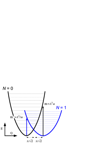
Figure 1: Schematic effective nuclear potential (cf. Eq. (5)) for the neutral ($N=0$, black) and charged ($N=1$, blue) electronic state of the molecule. The large charging energy has been subtracted since near the charge degeneracy point only changes in the vibrational energy are of importance for the differential conductance. The potentials are plotted as function of the normalized coordinate $Q$ (see text) and are relatively shifted by $\sqrt{2}\lambda>0$ and distorted by a factor $\alpha^{2}=\omega_{0}/\omega_{1}>1$. The vertical arrows indicate the change in the classical elastic energy when charging (blue) and de-charging (black) the molecule, respectively, while maintaining the nuclei at the equilibrium position of the initial charge state.

We consider a molecule which is weakly tunnel-coupled to a left (L), and right (R) metallic electrode and capacitively coupled to a gate electrode. The transport is assumed to be dominated by a single orbital on the molecule and double occupancy of this orbitals prohibited by strong Coulomb blockade. For simplicity we disregard effects of electron spin degeneracy (the minor quantitative corrections are trivial to include) so we can consider spinless non-interacting electrons. Nuclear motion internal to the molecule is taken into account through a single vibrational mode which couples both linearly and quadratically to the charge on the molecule. As mentioned above, quadratic coupling may certainly compete with linear effects. The Hamiltonian $H=H_{\rm{M}}+\sum_{r}H_{r}+H_{\rm{T}}$ incorporates the molecule ($\rm{M}$), reservoirs $r=L,R$ and the tunneling between molecule and electrodes ($\rm{T}$):

$$H_{\rm{M}} = \sum_{N=0,1}|N\rangle\langle N|H_{N},$$ (1)

$$H_{N} = \frac{p^{2}}{2M}+\frac{M}{2}\omega_{N}^{2}\left(x\pm\delta x/2\right)^{2},$$ (2)

$$H_{\rm{e}} = \sum_{r=R,L}\sum_{k}\epsilon_{kr}a_{kr}^{{\dagger}}a_{kr},$$ (3)

$$H_{\rm{T}} = \sum_{r=R,L}\sum_{k}t_{r}a_{kr}^{{\dagger}}|0\rangle\langle 1|+h.c.,$$ (4)

where $\pm$ corresponds to $|N\rangle$ denoting the neutral ($N=0$) and charged ($N=1$) electronic state of the molecule respectively. We employ units $\hbar=k_{B}=e=1$. The electrodes $r=L,R$ are described by the non-interacting Hamiltonian $H_{\rm{e}}$. They are maintained at fixed temperature $T$ and electrochemical potentials $\mu_{r}=\mu\pm V/2$, where $V$ is the applied bias voltage. The average chemical potential is defined such that $\mu=0$ corresponds to the charge degeneracy point (including the change in vibrational zero-point energy of the molecule). The gate voltage then effectively varies $\mu$ relative to the vibrational transition energies of the molecule. The Hamiltonians $H_{N},N=0,1$ describe the vibrational motion in the neutral and charged electronic state, respectively, which gives rise to the excitation spectra. This is depicted in Fig. 1. Here $x$ and $p$ ($[x,p]=i$) are the vibrational coordinate and momentum, respectively, and $M$ is the effective mass. Typically, in each charge state the lowest order approximation to effective nuclear potential around its minimum is a harmonic potential. Importantly, both the equilibrium position and frequency depend on the charge state, $\omega_{0}\neq\omega_{1}$ and $\delta x\neq 0$. Which effect will be more important depends on microscopic details of the molecule. Since the ZPMs are different it is not obvious how to define a single normalized coordinate. It is convenient to introduce the geometric-mean frequency $\Omega=\sqrt{\omega_{0}\omega_{1}}$ as the vibrational energy scale. We relate the shift to the dimensionless parameter $\lambda=\sqrt{M\Omega/2}\delta x$ and the frequency distortion to $\alpha=\sqrt{\omega_{0}/\omega_{1}}$ (i.e. $\omega_{0,1}=\alpha^{\pm}\Omega$). Using the dimensionless coordinate $Q=\sqrt{M\Omega}x$ normalized to the ZPM associated with $\Omega$ and the conjugate momentum $P$, $[Q,P]=i$ we rewrite $H_{N}$ in the form (see also A)

$$H_{N}=\frac{\omega_{N}}{2}\left[\frac{P^{2}}{\alpha^{\pm}}+\alpha^{\pm}\left(Q\pm\lambda/\sqrt{2}\right)^{2}\right].$$ (5)

with $\pm$ for $N=0,1$. We label the molecular eigenstates by $N_{m}$ and write their wave functions as $|N\rangle|m\rangle_{N}$, where $|m\rangle_{N}$ is the vibrational eigenstate with $m=0,1,2,...$ quanta excited on the potential surface for electronic state $|N\rangle,N=0,1$: $H_{N}|m\rangle_{N}=\omega_{N}(m+1/2)|m\rangle_{N}$. Different regimes are characterized by comparing the change in the classical elastic energies involved in the vertical transitions to each potential (see Fig. 1) with the vibrational frequency of the final charge state. (Equivalently one compares the ZPM of each potential with the relative shift of the two potentials.) The relevant dimensionless couplings are thus $\lambda^{2}\alpha\gtrless 1$ and $\lambda^{2}/\alpha\gtrless 1$. Due to the spatial inversion symmetry of each potential about its minimum the transport problem is invariant under $\lambda\rightarrow-\lambda$ and $(\alpha,\mu)\rightarrow(\alpha^{-1},-\mu)$ (see A). Therefore, assuming $\lambda\geq 0,\alpha\geq 1$ only three regimes need to be considered (i) $\lambda^{2}<1/\alpha$, (ii) $1/\alpha<\lambda^{2}<\alpha$, and (iii) $\alpha<\lambda^{2}$.
Transport. The tunneling of electrons with an excess energy provided by the bias voltage drives the molecule out of electronic and vibrational equilibrium. In the weak tunneling regime, i.e. $\Gamma\ll T$, the occupation probabilities $P^{N}_{m}$ for $N$ electrons on the molecule and $m$ vibrational quanta excited may be described by a stationary master equation. Neglecting for now relaxation of the vibrational states by the environment (see Sect. 2.2) we have:

$$\dot{P}_{m}^{0}=0 =\sum_{rm^{\prime}}\left(W_{0m\leftarrow 1m^{\prime}}^{r}P^{1}_{m^{\prime}}-W_{1m^{\prime}\leftarrow 0m}^{r}P^{0}_{m}\right),$$ (6)

$$\dot{P}_{m^{\prime}}^{1}=0 =\sum_{rm}\left(W_{1m^{\prime}\leftarrow 0m}^{r}P^{0}_{m}-W_{0m\leftarrow 1m^{\prime}}^{r}P^{1}_{m^{\prime}}\right),$$

with transition rates due to tunneling to/from electrode $r=L,R$

$$W_{1m^{\prime}\leftarrow 0m}^{r} = \Gamma^{r}F_{m^{\prime}m}f_{r}(\mu_{m^{\prime}m}),$$

$$W_{0m\leftarrow 1m^{\prime}}^{r} = \Gamma^{r}F_{m^{\prime}m}[1-f_{r}(\mu_{m^{\prime}m})].$$ (7)

where $f_{r}(E)\equiv(e^{(E-\mu_{r})/T}+1)^{-1}$. The addition energies for the transition $1_{m^{\prime}}\leftarrow 0_{m}$ are

$$\mu_{m^{\prime}m}=\omega_{1}m^{\prime}-\omega_{0}m=\Omega(\alpha^{-1}m^{\prime}-\alpha m).$$ (8)

and the Frack-Condon factors

$$F_{m^{\prime}m}=|_{1}\langle m^{\prime}|m\rangle_{0}|^{2}.$$ (9)

Where possible we will reserve $m$ and $m^{\prime}$ for vibrational numbers of the charge state $N=0$ and $N=1$, respectively. The stationary current flowing out of reservoir $r=L,R$ is given by

$$I_{r}=\sum_{mm^{\prime}}\left(W_{1m^{\prime}\leftarrow 0m}^{r}P_{m}^{0}-W_{0m\leftarrow 1m^{\prime}}^{r}P_{m^{\prime}}^{1}\right)$$ (10)

The probabilities are normalized, $\sum_{Nm}P^{N}_{m}=1$, and the current is conserved, $I_{L}+I_{R}=0$.
Spectral features. Due to the $\mu$ and $V$ dependence of the transition rates (7) the current will change whenever a resonance $\mu_{r}=\mu_{m^{\prime}m}$ is crossed. For $r=L,R$ this defines a line with negative/positive slope in $(\mu,V)$ plane for $V>0$ (which we consider from hereon) where a new electron tunneling process becomes possible. Here the molecule can change its vibrational energy by an amount $\mu_{m^{\prime}m}$. Without distortion ($\alpha=1$) this resonance condition only depends on the change in vibrational number $m^{\prime}-m$. For instance, once the transition $0_{0}\rightarrow 1_{k}$ is energetically allowed for some fixed integer $k$, transitions $0_{m}\rightarrow 1_{m+k}$ are allowed for all $m=1,2,\ldots$. This infinity of processes becomes energetically allowed at a single resonance line. In combination with other allowed transitions a cascade of transitions gives access to arbitrarily high excited states [19] and results in a divergence of the average phonon-number when we let $\lambda\rightarrow 0$ [16] for fixed applied voltages. For $\alpha\neq 1$ the mean of the two vibrational numbers also enters into the resonance condition since $\mu_{m^{\prime}m}/\Omega=(\alpha+\alpha^{-1})(m^{\prime}-m)/2-(\alpha-\alpha^{-1})(m+m^{\prime})/2$ The cascades of transitions are now switched on in a sequence of steps.
Intensities. The sign and intensity of the change in the current at the resonances is determined by the rates $\Gamma^{r}$ for tunneling to/from electrode $r=L,R$ and the Franck-Condon (FC) factors $F_{m^{\prime}m}$. The FC-factors take into account that the nuclear potential is altered when the molecule becomes charged. Their energy dependence through the vibrational numbers $m,m^{\prime}$ is typically dominant over that of the rates which we take to be constants $\Gamma^{r}=2\pi|t_{r}|^{2}\rho_{r}$ with density of states $\rho_{r}$ in electrode $r=L,R$. In contrast to most transport models, here the FC-factors are non-symmetric $F_{m^{\prime}m}\neq F_{mm^{\prime}}$. In general this is the case when the nuclear potentials in the two charge states are not identical up to a shift. The sum rules $\sum_{m}F_{m^{\prime}m}=\sum_{m^{\prime}}F_{m^{\prime}m}=1$ are due to the completeness of each vibrational basis set $\{|m\rangle_{0}\}$ and $\{|m^{\prime}\rangle_{1}\}$. These guarantee that the current and the total occupation $P^{N}=\sum_{m}P^{N}_{m}$ of each charge state $N$ will saturate at large bias voltage to the electronic limit (i.e. without the vibration) $I_{e}=(\sum_{r}1/\Gamma^{r})^{-1}$ and $P^{0,1}_{e}=\Gamma^{L,R}/(\sum_{r}1/\Gamma^{r})$, provided the FC-factors are bias voltage independent (cf. [9]).

2.1 Franck-Condon factors - Classical and quantum features

The FC-factors for any $\lambda$ and $\alpha$ can be calculated analytically by disentangling the unitary transformation which maps the oscillator $H_{1}$ onto the oscillator $H_{0}$. The expressions and their derivation are deferred to A and we will focus here on their essential features.

Figure 2: Franck-Condon factors in grayscale (black = 1,white=0). The quasi-classical boundary curves (yellow lines) separate classically allowed and forbidden transitions (see B). Sketched below each panel are the classical phase space $(Q,P)$ trajectories of the vibration in charge state $N=0$ (black) and $N=1$ (blue) with energy $m\omega_{0}$ and $m^{\prime}\omega_{1}$. The red numbers $(2)$ and $(4)$ in the grayscale plots indicate the number of intersections of these trajectories. (a) $\alpha=1,\lambda=3.0$. For strong shift, $\lambda^{2}\gg\alpha$ the FC-factors are suppressed for small $m^{\prime},m$ and exponentially increase as the classically allowed region is approached. (b) $\alpha=2.05,\lambda=3.0$. For combined shift and distortion the FC-factors are asymmetric in $m,m^{\prime}$ (although they are symmetric in the limiting cases (a) and (c) due to special symmetries). (c) $\alpha=2.05,\lambda=0$. For strong distortion, $\lambda^{2}\ll 1/\alpha$ the FC-factors rapidly decrease with $m,m^{\prime}$ and in addition oscillate due to the parity selection rule (checkerboard pattern).

In Fig. 2 we plot the FC-factors in gray-scale for three representative cases. Their large-scale dependence on the vibrational numbers $m,m^{\prime}$ follows from quasi-classical arguments as is discussed in detail in B. In the case of only a large shift ($\lambda^{2}>1,\alpha=1$, Fig. 2(a)), the FC-factors are basically nonzero only in a classically allowed region bounded by the so-called Condon parabola [21, 19]. The maximal values occurs at $m=\lambda^{2},m^{\prime}=0$ and $m=0,m^{\prime}=\lambda^{2}$. For $\lambda\rightarrow 0$ this parabola narrows down to a line, $F_{m^{\prime}m}\rightarrow\delta_{m^{\prime}m}$. For only a large distortion ($\alpha\gg 1,\lambda=0$, Fig. 2(c)), the classically allowed region has two linear boundaries (which coincide for $\alpha\rightarrow 1$) and the maximal value occurs for $m=m^{\prime}=0$. When both a shift and a distortion occur (Fig. 2(b)) the boundary curve is partially linear and partially parabolic. Additionally, two classically allowed regions of different intensity can be distinguished, corresponding to a difference in possible classical motions. The global maximum occurs for $m=0,m^{\prime}=\lambda^{2}/\alpha$ and a local maximum for $m=\lambda^{2}\alpha,m^{\prime}=0$, corresponding to the two different classical elastic energy scales. It is important to note that for $\alpha>1$ one can have a shift which is large relative to the ZPM of one potential ($\lambda^{2}\alpha>1$) but still small relative to the ZPM of the other ($\lambda^{2}/\alpha>1$). In this case interference effects may occur in the FC-factors which are directly observable in the electronic transport (see Sect. 3.2).
The distortion breaks the symmetry between the neutral and charged state in two respects: the vibrational excitation spectra of the neutral and charged state become asymmetric and the FC-factors become asymmetric as function of the energies $E_{m}=m\omega_{0},E_{m^{\prime}}=m^{\prime}\omega_{1}$ (not shown). Note that this is also the case for $\lambda=0,\alpha>1$, even though in this case $F_{m^{\prime}m}=F_{mm^{\prime}}$ (see Fig. 2(c)). Together these lead to a lack of inversion symmetry of the current with respect to the gate energy $\mu\rightarrow-\mu$ even in the case $\Gamma^{L}=\Gamma^{R}$.
The qualitative classical understanding of the FC-factors allows one to understand the dependence of the occupations and the current on the applied voltages in detail using figures like Fig. 2. This is discussed in C. For instance, for strong shifts ($\lambda^{2}\gg 1,\alpha=1$) one can explain the blockade of the current at low voltage [13], negative (NDC) instead of positive differential conductance (PDC), and even sharp current peaks [19] in terms of a feedback mechanism in the vibration-assisted transitions between the molecular states. The detailed variations of the FC-factors within the classically allowed region are not needed for this. Although the current steps at discrete energies are due to the quantized nuclear motion the variation of their sign and intensity follow from quasi-classical features of the FC-factors. However, when a distortion is present interference effects in the sign and intensity of the conductance resonances may appear. For instance, for purely distorted potentials ($\lambda=0$) the spatial inversion symmetry of the vibrational wave function cannot be changed by the electron tunneling. This leads to a strict parity-selection rule for the FC-factors (see A):

$$F^{\lambda=0}_{m^{\prime}m}=0~{}{\rm unless}~{}m^{\prime}-m={\rm even}$$ (11)

This is visible as a checkerboard pattern in Fig. 2(c). For weakly shifted but distorted potentials the tunneling rates can still vary significantly when the vibrational number changes by only one (see Sect. 3.2.1). This leads to even-odd effects in the intensity and sign of the conductance. For a intermediate shift of the potentials the decay rate of a single low-lying excited state can be coherently suppressed while its rate of population is coherently enhanced. This is possible only when the nuclear ZPM of the two potentials are sufficiently different. As a result the transport is suppressed in a large regime of applied voltages. Both effects require asymmetric excitation spectra i.e. a distortion. This indicates why interference effects in the FC-factors played no role in previous works.

2.2 Relaxation

The FC-factors strongly influence the type of non-equilibrium vibrational distribution which the transport current induces on the molecule . To be able to identify such effects qualitatively we compare our results with those where vibrational excitations on the molecule can relax by coupling to an environment of oscillators. For simplicity we assume that the spectral function of the environment is a constant $\gamma$ and the temperature is equal to that of the electrodes, $T$. For weak coupling to this environment, $\gamma\ll{\rm min}\left\{\omega_{N}\right\}$ , its influence can be included through an additional term $\sum_{n}(W_{Nm\leftarrow Nn}P^{N}_{n}-W_{Nn\leftarrow Nm}P^{N}_{m})$ to the right-hand side of equation (6) for $\dot{P}^{N}_{m}$ without altering the expression for the current (10). The rates are given by

$$W_{Nn\leftarrow Nm}=\gamma[\pm b(\omega_{N}(n-m))]$$ (12)

for $n\gtrless m$ and $N=0,1$ where $b(E)=(e^{E/T}-1)^{-1}=-(1+b(-E))$. The relaxation can be either strong ($\gamma>\Gamma$) or weak ($\gamma<\Gamma$) relative to the tunneling as long as both are smaller than $T$ and ${\rm min}\left\{\omega_{N}\right\}$. What is of interest here is that non-equilibrium effects of different physical origin disappear at different characteristic strengths of the relaxation $\gamma\lesssim\Gamma$ i.e. they have a specific sensitivity to relaxation processes. The case of strong relaxation will not be discussed except for the important fact that in this limit NDC effects vanish in any single orbital model regardless of the FC-factors [19]. This may be shown using an equilibrium ansatz for the vibrational distribution [10, 12]. Thus in limit of weak tunneling and weak coupling to the environment considered here NDC implies non-equilibrium.

3 Results

The stationary current $I$ (Eq. (10)) and differential conductance $dI/dV$ are presented for symmetric tunneling rates $\Gamma^{r}=\Gamma,r=L,R$ and temperature $T/\Omega=0.01$. Gray-scale plots of $dI/dV$ have different linear scale factors for $dI/dV\gtrless 0$ to clarify voltage conditions for which NDC effects occur. Their magnitudes can be appreciated from the presented $I(V)$ curves or from the text. We will consider parameter values which are well separated to keep the discussion simple. At this point a general conclusion can already be made: for all values of $\lambda$ for which we present results no NDC is visible if we set $\alpha=1$. The occurrence of NDC in all cases where $\alpha\neq 1$ indicates that a distortion enhances non-equilibrium vibrational effects, however via several different mechanism which we will now analyze.

3.1 Nearly symmetric excitation spectra: $\alpha^{2}<2$

For moderate values of $\alpha^{2}<2$ only one vibrational excitation of $N=1$ lies below the first one for $N=0$ (cf. Fig. 1). The low energy spectra in the two charge states may thus be characterized as nearly identical. Interestingly, due to the slight asymmetry the current provides direct information on the changes in vibrational distribution which remain hidden without a distortion. Some effects of interference in the FC-factors may be identified.

3.1.1 Small shift $\lambda^{2}\ll 1/\alpha,\alpha$: Broadening of the vibrational distribution

For $\alpha=1$ the $dI/dV$ is completely featureless apart from the ground-state transition lines. A distortion causes the ground-state resonance line to split in many excitation lines which can be resolved at low temperature, as can be seen in Fig. 3. The current, shown in Fig. 4, is strongly modulated on the new small energy scale $\omega_{0}-\omega_{1}$ by which the resonances are separated. This modulation is expected since the tunneling rates strongly decrease with increasing energy. The featureless result for $\alpha=1$ is rather special since it is due to the exact symmetry of the excitation spectra for $N=0$ and $N=1$.

Figure 3: Differential conductance for $\alpha=1.05,\lambda=0.01$. White and black relative to the grey background indicate positive and negative intensity of $dI/dV$. The same holds for all subsequent grayscale plots.

Figure 4: $I(V)$ normalized to the electronic limit $I_{e}$ for $\mu/\Omega=1.5$ in Fig. 3. The current steps are spaced by the frequency difference $\omega_{0}-\omega_{1}$.

Figure 5: Transitions relevant to the right in Fig. 3. In all this kind below black/blue levels correspond to ground- and excited vibrational states of the neutral/charged molecule, $0_{m},m=0,1,2,\ldots$/ $1_{m^{\prime}},m^{\prime}=0,1,2,\ldots$. The parity of the states is indicated by the line style (full=even, dashed=odd). Arrow thickness indicates the relative strength of the FC-factors. Parity forbidden/allowed transitions are indicated by a full/dashed arrow. Not all transitions are indicated. (a) For $\mu_{L}>2\omega_{1}$ all grey transitions are energetically allowed and only the missing links (green) in the cascade need to be switched on, one by one starting from below, at the resonance lines $-\mu_{R}=k(\omega_{0}-\omega_{1})$ for $k=1,2,\ldots,[1/(\alpha^{2}-1)]+1$. After the last transition is possible the scheme repeats for the higher lying states i.e. all states are energetically accessible and a broad vibrational distribution is established. (b) For $2\omega_{1}>\mu_{L}>\omega_{1}$ the progression does not occur due to the parity effect.

The progression of lines maps out the stepwise lengthening of cascades of transitions (Fig. 5(a)). Once $[1/(\alpha^{2}-1)]+1$ ($[x]=$ integer remainder of $x$) of such resonances have been traversed (more than $2$ for $\alpha<\sqrt{2}$) , the cascade is infinitely long i.e. any state can be reached. This is the case for $-\mu_{R}>\omega_{0}$. The broadening of the vibrational distribution is thus sharply controlled by the bias voltage in this region. The individual processes which lead to the broad non-equilibrium vibrational distribution for $\lambda\ll 1$, discussed in [16], may thus be identified in the transport current if the vibrational excitation spectrum is charge dependent due to a distortion. From Fig. 2(c) one sees that for finite $\alpha$ the FC-factors do not collapse onto a line $F_{m^{\prime}m}=\delta_{m^{\prime}m}$ as we let $\lambda\rightarrow 0$. We therefore argue that the scaling of the vibrational distribution width found for $\alpha=1$ in [16] may break down for $\alpha\neq 1$ below some cut-off value for $\lambda$ (which depends on $\alpha$).
For $2\omega_{1}>\mu_{L}>\omega_{1}$ the progression seems to break down after the first large step. This is due to the suppression of all rates between even and odd excitations cf. Eq. (11), as Fig. 5(b) illustrates. Except for one sharp feature and a weak NDC effect the resonance lines corresponding to quasi-forbidden transitions are missing. Pronounced NDC occurs when the region $\mu_{L}>\omega_{1},\omega_{0}-\omega_{1}>-\mu_{R}$ is reached: the change in the current is $1/3$ of its maximal value. The occupation of state $1_{1}$ via a quasi-forbidden transition causes the drop in current since the probability is redistributed over the three states $0_{0},1_{0}$ and $1_{1}$ and the latter does not contribute to the current since $F_{10}\ll F_{00}$. Once the transition $0_{1}\leftarrow 1_{1}$ is energetically allowed all excited states are de-populated due to the quasi-selection rule for the FC-factors: $F_{10}\ll F_{11}$. The current nearly reaches its maximal value $\Gamma/2$. For $\lambda^{2}\lesssim 1/\alpha$ the selection rule is sufficiently weakened that the progression already starts at $\mu_{L}=\omega_{1}$ as seen in Fig. 6.

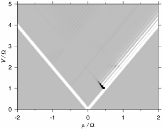
Figure 6: Differential conductance for $\alpha=1.05,\lambda=0.1$.

The progression is a non-equilibrium effect as it consists only of transitions between excited states. The number of visible lines is indicative of the average vibrational number and is reduced when a relaxation rate $\gamma>0$ is switched on (not shown). We point out that in Fig. 3 the energy separation in this progression of excitations could be mistaken for a vibrational frequency. Also one might infer erroneously a coupling $\lambda\lesssim 1$ since many resonances with decreasing intensity can be resolved. In fact the extent of the progression shows an dependence on the shift opposite to that of a usual FC-progression: it becomes shorter with increasing $\lambda$. Crucial for a correct identification are furthermore the featureless low bias region ($|\mu_{r}|<\omega_{0},\omega_{1}$) and the NDC effects.

3.1.2 Large shift $1/\alpha,\alpha\ll\lambda^{2}$: Trapping in the vibrational ground state

For strong shift the parity of the nuclear wave functions plays no role: in Fig. 7 resonance lines $\mu_{L}=m\omega_{1}$ and $-\mu_{R}=m\omega_{1}$ for $m=$ odd are now clearly visible.

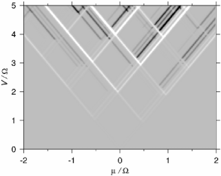
Figure 7: Differential conductance for $\alpha=1.05,\lambda=3.0$.

Figure 8: $I(V)$ normalized to the electronic limit $I_{e}$ for $\mu/\Omega=0.5$ in Fig. 7. We note that the average vibrational number shows the same marked peak as function of the bias voltage.

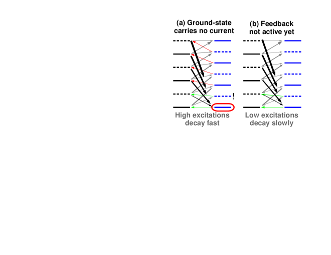
Figure 9: Transitions relevant to the right in Fig. 7. As in Fig. 5 the missing links (green and red) in the cascade are switched on. However, in this case the molecule becomes trapped in the ground states (not contributing to the current) for most applied voltages: once excited states become slightly occupied they feed back strongly into the ground state (black arrows) since the transition rates exponentially increase with the difference in vibrational energy (opposite to Fig. 5), see Fig. 2. Due to the gate asymmetry, $\mu>0$, the ground state can only decay via processes with much smaller rates. Due to the distortion of the spectrum this feedback mechanism is not yet active at the first two resonances (green arrows), causing the current to “overshoot” resulting in the marked peak in Fig. 8.

For $\alpha=1$ a strong shift $\lambda^{2}\gg 1$ of the potentials is well-known to suppress the ground state transition line [22, 12, 13] and redistribute the weight into a FC-progression of conductance resonances. At this point it should be emphasized that the suppression is a non-equilibrium effect even though the vibrational distribution has its main weight in the ground states. This is evidenced by the disappearance of the NDC and current peaks [19] which occur for values of $\lambda\gtrsim 4$ and asymmetric gate energy ($|\mu|>\omega$) and the enhancement of the suppression [13] upon full vibrational equilibration.
The main effect of the distortion comes from the asymmetric spectrum. What is remarkable in Fig. 7 compared to Fig. 3 is that most of the resonances at higher bias with spacing on the small scale $\omega_{0}-\omega_{1}$ lead to NDC, whereas the excitations on the larger scale $\omega_{0},\omega_{1}$ all correspond to PDC. The same cascade of transitions discussed in Sect. 3.1.1 now stabilizes the lowest vibrational states [19] which contribute little to the current. However, due to the small mismatch of the excitation spectra the current can first reach a high value which is subsequently reduced to the value it has for $\alpha=1$ when the cascades are switched on, see Fig. 8. This happens repeatedly with increasing bias. The effect here should thus not be characterized as current suppression. Rather, the current is enhanced relative to the case $\alpha=1$ where the feedback always dominates the current. Due to the slightly asymmetric spectra the trapping in the ground state is “postponed”. Markedly, the NDC lines have positive/negative slope for $\mu\gtrless 0$ which is opposite to that of the NDC occurring for very large $\lambda$ and $\alpha=1$ [13, 19].

3.2 Asymmetric spectra: $\alpha^{2}>2$

For sufficient distortion, $\omega_{0}>2\omega_{1}$, two or more excitations of the $N=1$ charge state lie below the first excitation in the $N=0$ state i.e. there is a true asymmetry between the spectra of the two charge states. This brings about a simplification: most of the features discussed below are qualitatively reproduced when truncating the spectrum at energies above the larger vibrational frequency $\omega_{0}$, retaining only the states $m=0,1$ and $m^{\prime}=0,\ldots,[\alpha^{2}]+1$ for $N=0$ and $N=1$ respectively. Due to the presence of the $N=1$ low-lying states interference effects in the FC-factors also gain importance. For small shift the quasi-conservation of the nuclear wave function parity suppresses the electron tunneling between all even and odd vibrational states of $N=0$ and $N=1$. For larger shifts $\lambda^{2}\gtrsim 1/\alpha$ interference may suppress the decay rate of a single low-lying excitation and simultaneously enhance the rate at which this state is populated. This concerted effect of constructive and destructive interference is due to the opposite parity of the $N=0$ vibrational ground- and excited state.

3.2.1 Small shift $\lambda^{2}\ll 1/\alpha$: Parity effect

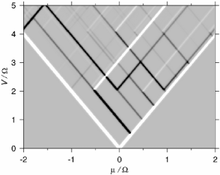
Figure 10: Differential conductance for $\alpha=2.05,\lambda=0.01$.

Figure 11: $I(V)$ normalized to the electronic limit $I_{e}$ for $\mu/\Omega=0.1$ in Fig. 10. The first three current plateaus values are describe by Eq. (13). In particular, for $\alpha^{2}\gg 1$ the initial current drop by a factor 1/3 signals the redistribution of the probability from two to three states.

Figure 12: Transitions relevant to the parity effects in Fig. 10. The closely spaced excitations belong to charged state $N=1$, the levels with large spacing (only two shown) belong to $N=0$. (a) Successive occupation of the non-contributing states $1_{m^{\prime}}$ leads to NDC lines at low bias. The variation of the NDC intensity reflects wether the transition is parity forbidden (dashed line) or allowed (full line). (b) The successive opening of escape processes (green and red arrows) from the states not contributing to the current gives PDC for even and NDC for odd excitations.

The $dI/dV$ in Fig. 10 has two distinctive features. Below the threshold voltage where $0_{1}$ can not yet be reached (horizontal zig-zag line), all resonance lines (with negative slope) correspond to NDC with an intensity which alternates. Above the threshold resonances lines (with positive slope) appear with alternating sign of the differential conductance. Both effects derive from the parity quasi-selection rule incorporated in the FC-factors and are systematic: as one increases $\alpha^{2}$ by one, the additional resonances appearing below and above the threshold voltage follow the above pattern. We explain this parity effect using Fig. 12.
NDC intensity alternation. All the low voltage resonances correspond to NDC since the low-lying excitations of $N=1$ become successively occupied (Fig. 12(a)) without contributing significantly to the current (the FC-factors $F_{m^{\prime}0}$ rapidly decrease with $m^{\prime}$). Since the rates at which each excitation is populated and depleted are the same (although small), the ground state occupation is reduced $\propto 1/V$ resulting in a lower current at higher bias. However, the FC-factors $F_{m^{\prime}0}$ also oscillate: transitions from the ground state $0_{0}$ to odd-$m^{\prime}$ states $1_{m^{\prime}}$ are strongly suppressed relative to those with even $m^{\prime}$, $F_{(2n+1)0}\ll F_{(2n)0}$ for $n=1,2,\ldots$. Remarkably, the quasi-forbidden transitions appear as anti-resonances in the differential conductance (instead of missing resonances) which modulate the current stronger than allowed transitions. This effect is related to the non-equilibrium conditions (see below). This may be explicitly demonstrated from the expression for current plateau $k=1,2,\ldots$ where $k\propto V$

$$I_{k}=\left[(k+1)/\Gamma^{R}+1/\Gamma^{L}\right]^{-1}\sum_{m^{\prime}=0}^{k}F_{m^{\prime}0}.$$ (13)

This result applies at low bias where states $m=0$ and states $m^{\prime}\leq k$ are occupied and state $0_{1}$ is not yet reachable (Fig. 12(a)). For $\Gamma^{r}=\Gamma$ the current after an initial big step decreases $\propto 1/V$, since the number of occupied excited levels which do not contribute to the current grows $\propto V$. Interestingly, for asymmetric coupling to the electrodes $\Gamma^{L}\ll\Gamma^{R}$ the depletion of the ground states is postponed: the current initially increases in steps with $V$ to reach a maximum around $V\propto\omega_{1}(\Gamma^{R}/\Gamma^{L})$ and then decays $\propto 1/V$. For negative bias the current shows no such maximum.
NDC / PDC alternation. From the low bias resonances one can directly find the FC-factors if the tunneling rates $\Gamma^{L,R}$ are known. However, above the threshold voltage this is not the case anymore: here multiple states from both charge sectors contribute in a more complicated way (Fig. 12(b)). Now escape from the non-contributing states $1_{m^{\prime}}$ becomes possible. Remarkably, this suppresses the current further at lines with positive slope terminating at the NDC resonances due to quasi-forbidden transitions. This is due to a feedback mechanism in the vibration assisted transitions which effectively traps the system in the odd-parity states as explained in Fig. 12. This is somewhat similar to the mechanism in the opposite case of strong shifts (Sections 3.1.2 and 3.2.3) but relies critically on the modulation of the rates due to the quasi-conservation of parity.

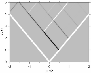
Figure 13: Differential conductance for $\alpha=2.05,\lambda=0.01$ and finite relaxation rate $\gamma/\Gamma=0.1$. At this intermediate value of the relaxation only the odd NDC lines are suppressed, cf. Fig. 10. The spacing between the remaining even resonance lines with negative slope may be mistaken for the vibrational frequency of the excitations i.e. they mimic an effective frequency doubling. However, the resonance lines with positive slope are inconsistent with such an interpretation and hint at the missing resonances due to the parity effect.

The allowed and forbidden excitation lines have different sensitivity to relaxation processes and disappear in two stages. When increasing the relaxation rate $\gamma$, in a first stage the strong NDC effects due to quasi-forbidden transitions become comparable in intensity with the NDC due to allowed ones and subsequently disappear as shown in Fig. 13. Thus similar to optical spectroscopy the parity selection rule now leads to missing resonances in the spectrum. The alternation of the sign of the resonances above the threshold voltage also disappears since it is caused by asymmetries in the smallest rates. Only in a second stage the remaining NDC lines due to the $m^{\prime}=$even states disappear.

3.2.2 Intermediate shift $1/\alpha<\lambda^{2}<\alpha$: Coherent suppression

Interestingly for any $\alpha>\sqrt{2}$ a drastic suppression of the current occurs near special values of $\lambda$, a prominent example being

$$\lambda_{(2)}=\frac{1}{2}\sqrt{\alpha-\frac{1}{\alpha^{3}}}.$$ (14)

As seen in Fig. 14 at large voltage bias the current is completely suppressed beyond the ground-state transition line $\mu_{R}=0$. In this region the low-lying excited state $1_{2}$ becomes completely occupied i.e. we have a bias driven population inversion between vibrational states (cf. [19]). The reason for this is twofold and is explained in Fig. 15(b): due to destructive interference the rate of decay to the ground state $0_{0}$ is suppressed (FC-factor $F_{20}=0$ for $\lambda=\lambda_{(2)}(\alpha)$); simultaneously constructive interference maximizes the tunneling rate into this state from the excited state $0_{1}$. This concerted effect is due to the opposite parity of the ground- and excited state for $N=0$. As soon as the excited state $0_{1}$ can be reached via some tunneling processes the excited state $1_{2}$ becomes fully occupied and suppresses the transport. This happens at the bias voltage threshold forming the horizontal zig-zag line which we encountered above. The transport is recovered only when direct escape ($1_{1}\leftarrow 0_{2}$) from the coherently blocked state becomes energetically allowed i.e. $-\mu_{R}>\omega_{0}-2\omega_{1}$ (strong white line with positive above the suppressed region in Fig. 14). The effect is coherent in the sense that both destructive and constructive interference of the nuclear wave function are responsible for the suppression of electron transport through the molecule.

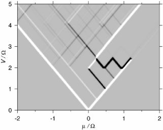
Figure 14: Differential conductance for $\alpha=2.05,\lambda=0.7$.

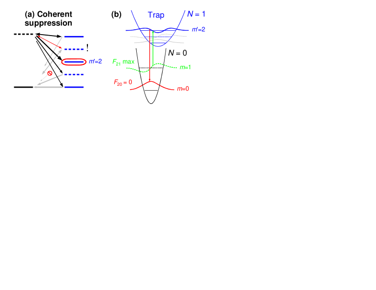
Figure 15: (a) Transitions relevant to the coherent suppression of the current on the right in Fig. 14. The decay rate of excited state $1_{2}$ to the ground state $0_{0}$ is suppressed due to destructive interference in the nuclear wave function overlap. State $1_{2}$ can thus not be reached directly, but due to the asymmetric spectra it can reached in three tunneling process via the excitations above it and the excited state $0_{1}$ (for $V$ above the zig-zag threshold in Fig. 14). The rate for the last process, $0_{1}\rightarrow 1_{2}$ is maximized due to constructive interference. The coherently enhanced ratio of rates for going in and out of $1_{2}$ suppresses the current. (b) Nuclear wavefunction overlap for $\lambda=\lambda_{(2)}$: the maximum and node of the states $0_{0}$ and $1_{0}$, respectively, align with the node of excitation $1_{2}$, thereby creating a low-energy blocking state.

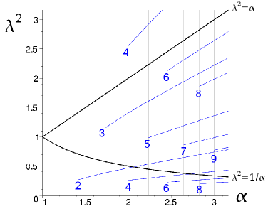
Figure 16: Conditions for coherent suppression in the $(\alpha,\lambda^{2})$ plane. Regimes of weak ($\lambda^{2}<1/\alpha$), intermediate ($1/\alpha<\lambda^{2}<\alpha$), and strong shift ($\alpha<\lambda^{2}$) are separated by black boundary lines. The blue curves labeled by integers $m^{\prime}$ indicate the values of $\lambda$ for which the FC-factor $F_{m^{\prime}0}$ vanishes for fixed $\alpha$. The curves are plotted only for those values of $\alpha$ for which state $m^{\prime}$ lies below the first excitation of $N=0$ charge state and where the coherent suppression occurs.

In a similar way, the FC-factor $F_{m^{\prime}0}$ of a higher excited state $1_{m^{\prime}},m^{\prime}=3,4,\cdots$ may vanish for some value of $\lambda$. (For $m^{\prime}=1$ this happens only for the trivial value $\lambda=0$.) If in addition this state lies below the first excitation for $N=1$, i.e. $\alpha^{2}>m^{\prime}$, this leads to a region of suppressed current similar in shape to that in Fig. 14 but more narrow (e.g. for $m^{\prime}=3$ the width of the region is halved). The lines in the $(\alpha,\lambda^{2})$-plane where both these conditions for the coherent suppression are satisfied are plotted in Fig. 16 for $m^{\prime}=2-9$. The curves are all of the form Eq. (14) but with a prefactor which differs from $1/2$. The region where this interference effect occurs is centered around the regime $1/\alpha<\lambda^{2}<\alpha$ and $\alpha>\sqrt{2}$, where it is possible to have a shift which is larger than the ZPM of the flattest potential but still smaller than that of the steepest potential. With increasing $\alpha$ the values of $\lambda$ where the coherent suppression occurs start to abound and even proliferate into the regime where the shift becomes strong, $\lambda^{2}>\alpha$, see Fig. 16. With increasing $\alpha$ the number of such values rapidly increases roughly $\propto\alpha^{4}$: since state $1_{m^{\prime}}$ has $m^{\prime}$ nodes there are $[m^{\prime}/2]$ zeros of $F_{m^{\prime}0}$ as a function of $\lambda$ for a given $\alpha$ and only the states $m^{\prime}=2,\cdots,[\alpha^{2}]$ have energy $<\omega_{0}$. Finally, we note that excited states with $m^{\prime}>[\alpha^{2}]$ are not expected to cause a coherent suppression effect since they always have two (groups of) states with opposite parity to decay to. It is highly unlikely that the decay rates to both types of states can be suppressed simultaneously by a special choice of the shift $\lambda$.
Naturally the coherent effect is more sensitive to parameter values than the quasi-classical trapping effect (cf. Sect. 3.1.2 and 3.2.3). This sensitivity has an interesting side to it. (The effect of voltage dependence of $\lambda$ on the trapping effect was considered in [9].) Introducing only a weak dependence of the parameters, for instance $\lambda$, on the bias voltage, the current exhibits a pronounced dip down to zero when tuning the parameters $\alpha$ and $\lambda$ with $V$ through the condition for coherent suppression (14). In view of the many situations where this effect can occur (Fig. 16) this is an interesting novel possibility to be explored in single molecule devices.
Similar to the parity effect, introducing relaxation affects the transport in two stages. First the suppressed groundstate transition line is restored and the forbidden transition line disappears as depicted in Fig. 17. An NDC effect related to the state with the suppressed FC-factor is still present. In a second stage this effect also vanishes.

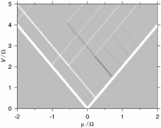
Figure 17: Differential conductance for $\alpha=2.05,\lambda=0.7$ and relaxation rate $\gamma/\Gamma=0.1$. Note that the excitation line of state with suppressed FC-factor is now missing and that the NDC at the zig-zag is weakened and moved to the straight line $\mu_{L}=3\omega_{1}$.

Excited states $m^{\prime}<[\alpha^{2}]$ have effective decay rate $\approx(m^{\prime}-1)\gamma$ and are therefore more sensitive to relaxation. In summary: of all the excitations $1_{m^{\prime}}$ the state $m^{\prime}=2$ gives rise to the strongest coherent suppression effect in the largest voltage region and is the least sensitive to relaxation.

3.2.3 Large shift $\lambda^{2}>\alpha$: Trapping in the vibrational ground state

Figure 18: Differential conductance for $\alpha=2.05,\lambda=3.0$. Note that the first excitation now leads to PDC, cf.Fig. 7.

Figure 19: $I(V)$ normalized to the electronic limit $I_{e}$ for $\mu/\Omega=1.25$ in Fig. 18.

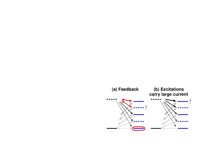
Figure 20: Transitions relevant to the NDC effects on the right in Fig. 18. (a) For most bias voltages transitions are switched on (red arrows) which eventually feed back (black arrows) into the vibrational ground state $1_{0}$ . Escape from the highest states $[\alpha^{2}],[\alpha^{2}]-1,\ldots$ with largest contributions to current becomes possible first, leading to the strongest NDC. (b) At the ground state transition line all the excitations $1_{m^{\prime}},m^{\prime}=1,\ldots,[\alpha^{2}]$ initially become occupied (gray arrows) and contribute to the a relatively large current without the feedback occuring.

The strong asymmetry between the excitation spectra due to the distortion results in the pronounced asymmetric conductance plot in Fig. 18. As one approaches the strong shift regime the NDC at resonances $\mu_{L}=m^{\prime}\omega_{1},m^{\prime}=1,\ldots,[\alpha^{2}]$ discussed below (Fig. 10) turns into PDC (cf. the first excitation in Fig. 14) and becomes suppressed in intensity at low bias for $\lambda^{2}>\alpha$ as seen in Fig. 18. This is also described by Eq. (13) (which holds for any $\lambda$) since the FC-factors increase with $m^{\prime},m$ for $\lambda^{2}>\alpha$, cf. Fig. 2(b). For negative gate energy $\mu$ the current slowly increases, but for positive $\mu$ the current surprisingly shows a sharp increase followed by NDC, despite the strong shift. Fig. 20 explains how the postponement of the classical trapping effect (similar to that discussed in Sec. 3.1.2) allows for large current steps despite the strongly shifted potentials. This results in strong PDC excitations spaced by the larger frequency $\omega_{0}$ and in between several pronounced NDC excitations with smaller spacing $\omega_{1}$ (in contrast to Fig. 7 where the NDC spacing is $\omega_{0}-\omega_{1}$).

4 Discussion

We have found that non-equilibrium vibrational effects are enhanced in molecular devices for which the effective potential for vibrations is sensitive to the charge state of the device. We modeled this by a change in the vibrational frequency in addition to a shift of the potential minima. In particular, for weak distortion of the potential the current was shown to map out sharp changes in the vibrational distributions with bias voltage. For sufficiently strong distortion of the potential interference effects of the nuclear wave functions were show to strongly influence the electron transport. The coherent effects are also expected to occur for more detailed models of the nuclear potentials since the requirements on the low-energy vibrational excitations are rather basic. The parity effect requires potentials which are distorted and only slightly shifted. The coherent suppression due to the vanishing overlap between an vibrational excited- and ground-state corresponding to a different charge on the molecule, requires a moderate shift and distortion. The precise conditions for the suppression will be different but Fig. 16 provides the qualitative picture. These mechanism, together with possible weak dependence on current or voltages offer interesting possibilities for controlling electron transport in single molecule devices.

Appendix A Franck-Condon factors for shifted and distorted potentials

In this Appendix we give the expressions for the FC-factors for potentials exhibiting both a relative shift and distortion. The derivation can be done by straightforward algebra without recourse to special functions (cf. [23, 24, 25]). We first note that the sign of the shift is irrelevant since the each of the states in the overlap integral has a definite parity with respect to spatial inversion relative to the minimum of its potential. Using this we find that interchanging $\omega_{0}\leftrightarrow\omega_{1}$ (i.e. $\alpha=\sqrt{\omega_{0}/\omega_{1}}\rightarrow\alpha^{-1}$ is equivalent to charge conjugation $N\rightarrow 1-N,N=0,1$ or $\mu\rightarrow-\mu$. We can thus restrict ourselves to $\alpha>1$ as long as we discuss both polarities of $\mu$. For the calculation of $F_{m^{\prime}m}$ it is convenient to normalize the coordinate to ZPM of the potential in question, $Q_{N}=x\sqrt{M\omega_{N}}$ and its conjugate $P_{N}$:

$$H_{N} = \frac{\omega_{N}}{2}\left[P_{N}^{2}+\left(Q_{N}\pm\sqrt{\alpha^{\pm}/2}\lambda\right)^{2}\right]$$ (15)

where $N=0,1$ corresponds to $\pm$ and the shift parameter is $\lambda=\sqrt{{M\Omega}/{2}}\delta x$ and the mean frequency $\Omega=\sqrt{\omega_{0}\omega_{1}}$. We obtain oscillator 1 from oscillator 0 by first applying a shift and then a distortion:

$$Q_{1} = \frac{Q_{0}}{\alpha}+\sqrt{2}\frac{\lambda}{\sqrt{\alpha}}$$

We write the corresponding transformation of the lowering operators, $b_{N}=\left(Q_{N}+iP_{N}\right)/\sqrt{2}$,

$$b_{1} = \frac{1}{2}\left(\frac{1}{\alpha}+\alpha\right)b_{0}+\frac{1}{2}\left(\frac{1}{\alpha}-\alpha\right)b_{0}^{{\dagger}}+\frac{\lambda}{\sqrt{\alpha}},$$

as a unitary transformation $b_{1}=e^{-S}b_{0}e^{S}$, where

$$S = \ln\alpha\left[\frac{1}{2}\left(b^{2}_{0}-b_{0}^{{\dagger}2}\right)-\frac{\lambda}{\sqrt{\alpha}-\frac{1}{\sqrt{\alpha}}}\left(b_{0}-b_{0}^{{\dagger}}\right)\right].$$

The exponential can be disentangled by the methods described in [26]: $e^{-S}=e^{Lb^{{\dagger}2}+lb^{{\dagger}}}e^{\left(\ln C\right)\left(b^{{\dagger}}b+\frac{1}{2}\right)+c}e^{Rb^{2}+rb}$ where the parameters in the exponential factors are

$$\left.\begin{array}[]{l}R\\ L\end{array}\right\}=\pm\frac{\alpha^{2}-1}{2\left(\alpha^{2}+1\right)},\left.\begin{array}[]{l}r\\ l\end{array}\right\}=\mp\frac{\lambda}{\alpha^{\pm 1/2}}\frac{2\alpha}{\alpha^{2}+1},C=\frac{2\alpha}{\alpha^{2}+1},c=-\lambda^{2}\frac{\alpha}{\alpha^{2}+1}.$$

The FC-factors $F_{m^{\prime}m}=|{}_{1}\langle m^{\prime}|m\rangle_{0}|^{2}=|{}_{0}\langle m|e^{-S}|m^{\prime}\rangle_{0}|^{2}$ are then directly found from the matrix elements

$${}_{0}\langle m|e^{S}|m^{\prime}\rangle_{0} = \sum_{k=0}^{\min\left\{m,m^{\prime}\right\}}\Theta_{mk}\left(L,l\right)\Theta_{m^{\prime}k}\left(R,r\right)C^{k+\frac{1}{2}}e^{c}$$

$$\Theta_{mk}\left(R,r\right) = \sqrt{\frac{m!}{k!}}\sum_{s=0}^{\left[\frac{m-k}{2}\right]}\frac{R^{s}r^{m-k-2s}}{s!\left(m-k-2s\right)!}$$

$$= \sqrt{\frac{m!}{k!}}\left(-ir\right)^{\left(m-k\right)}H_{m-k}\left(i\frac{r}{2R}\right)\left(\frac{R}{r^{2}}\right)^{\left[\frac{m-k}{2}\right]}$$

For $\alpha=1$ one obtains the well-known expression $F^{\alpha=1}_{m^{\prime}m}=e^{-\lambda^{2}}\frac{m!}{{m^{\prime}}!}\lambda^{2|m-m^{\prime}|}\left[L^{|m-m^{\prime}|}_{m}(\lambda^{2})\right]^{2}$ where $L$ is the associated Laguerre-polynomial and $m<m^{\prime}$ and $F_{m^{\prime}m}=F_{mm^{\prime}}$. For $\lambda=0$ the selection rule Eq. (11) is easily verified. The nonzero matrix elements, for instance, for the special case $m=0,m^{\prime}=2k$ are $F_{2k0}=\sqrt{1-\xi^{2}}\frac{(2k-1)!!}{(2k)!!}\xi^{2k}$ where $(2k)!!=(2k)(2k-2)\cdots 2$ , $(2k-1)!!=(2k-1)(2k-3)\cdots 1$ and $\xi=\frac{\alpha^{2}-1}{\alpha^{2}+1}$. The expression in terms of the Hermite polynomials $H_{n}$ reduces to the known result for $m^{\prime}=0,m\neq 0$ [24, 25].

Appendix B Classical features of the FC-factors

The large scale variations of the FC-factor $F_{m^{\prime}m}$ in the $\left(m,m^{\prime}\right)$ plane and their effects on the transport have a simple classical interpretation. It is important to discuss these if one wants to identify quantum effects of the nuclear motion. The central point is that the FC-factor becomes exponentially suppressed unless the nuclear motions in the effective potentials of the two charge states are compatible i.e. the phase-space trajectories of the two motions intersect. The boundary between classically forbidden and allowed regions in the $(m,m^{\prime})$-plane is found by requiring that the simultaneous equations (cf. Eq. (5))

$$\frac{1}{\alpha}P^{2}+\alpha\left(Q-\frac{\lambda}{\sqrt{2}}\right)^{2} = 2m$$

$$\alpha P^{2}+\frac{1}{\alpha}\left(Q+\frac{\lambda}{\sqrt{2}}\right)^{2} = 2m^{\prime}$$ (16)

have at least one real valued solution for $(P,Q)$ (the vibrational energies are $E_{0}=\omega_{0}m$ and $E_{1}=\omega_{1}m^{\prime}$). Within the classically allowed region there may be regions of different overall intensity related to the appearance of additional solutions. The intersections of the elliptic orbits determined by Eq. (16) are illustrated in Fig. 2. In the case of shifted potentials, $\lambda>0,\alpha=1$, $Q$ always has a single real solution. Two real solutions for $P$ exist if

$$m+m^{\prime}\geq\frac{1}{2}\left[\lambda^{2}+\frac{1}{\lambda^{2}}\left(m-m^{\prime}\right)^{2}\right]$$ (17)

This parabola in the $\left(m,m^{\prime}\right)$ plane, tilted by an angle $\pi/4$ relative to $m^{\prime}$ axis, is the so-called Condon-parabola [21] depicted in Fig. 2(a). The condition (17) is equivalent to demanding that the classical turning points of the two motions are interspersed. In the case of distorted potentials, $\lambda=0,\alpha>1,$ the requirement is

$$\frac{1}{\alpha^{2}}\leq\frac{m^{\prime}}{m}\leq\alpha^{2}$$ (18)

and real solutions are always four in number. The left inequality ensures that $Q$ is real. The corresponding lower boundary line in Fig. 2(c) is equivalent to requiring the potential energies of the motions are equal at the maximal coordinate ($P=0$). The right inequality ensures a real solution for $P$ and corresponds to equal kinetic energy at $Q=0$ (i.e. not at the classical turning point). For the general case $\lambda>0,\alpha>1$ two real solution exist for $P$ when $m,m^{\prime}$ lie inside a Condon-parabola

$$m\frac{1}{\alpha}+\alpha m^{\prime}>\frac{1}{2}\left[\lambda^{2}+\frac{1}{\lambda^{2}}\left(m\frac{1}{\alpha}-\alpha m^{\prime}\right)^{2}\right]$$ (19)

which is tilted by the angle $\varphi$ relative to $m$ axis, where $\tan\varphi={\alpha^{-2}}={\omega_{1}}/{\omega_{0}}$ i.e. the parabola tilts towards the axis corresponding to the highest frequency. It touches the axes at $m=\lambda^{2}\alpha$ and $m^{\prime}=\lambda^{2}/\alpha$, respectively, corresponding to the elastic energies. The solutions for $Q$ are always real in this region. However, an additional two real solutions for $Q$ occur between the parabolic boundary and below the line

$$m^{\prime}=\alpha^{2}m+\frac{\alpha^{3}}{\alpha^{4}-1}\lambda^{2},$$ (20)

beyond its tangent point with the parabola, which is located at $m=(\lambda^{2}\alpha)/(\alpha^{4}-1)^{2},m^{\prime}=(\lambda^{2}/\alpha)/(1-\alpha^{-4})^{2}$. In Fig. 2(b) one sees that in this region the FC-factors are clearly enhanced. The above classical expressions thus give an simple guide to the large scale structure of the complicated exact expression (A). For $\lambda\rightarrow 0$ the parabola (19) becomes very narrow and reduces to a line through the origin line $m^{\prime}/m=1/\alpha^{2}$, i.e. we recover Eq. (18). For $\alpha\rightarrow 1$ the region with 4 solutions moves to infinity with the tangent point of the parabola and we retain (17).

Appendix C Vibrational distribution and numerical convergence

Much of the behavior of the occupations $P^{N}_{m}$ and the current as function of the applied voltages may be understood from a simple scheme which is readily extended to situations with multiple competing orbitals [19]. First, to determine which direct transitions between states relevant one draws the region $\mu_{R}/\Omega<m^{\prime}/\alpha-m\alpha<\mu_{L}/\Omega$ (“bias window”) into the grayscale plot of the FC-factors. For $m^{\prime},m$ within this region transitions $1_{m^{\prime}}\leftrightarrow 0_{m}$ are both allowed whereas above/below this region only $1_{m^{\prime}}\rightarrow 0_{m}$ / $1_{m^{\prime}}\leftarrow 0_{m}$ is allowed by electrons leaving / entering the molecule via both tunnel junctions. Importantly, $m^{\prime},m$ outside the classically allowed region can be disregarded. In a second step we have to determine which states will become occupied significantly via cascades of tunnel processes (unless the relaxation is extremely fast, $\gamma\gg\Gamma$, in which case we can solve Eq. (6) using the vibrational equilibrium ansatz [10, 12]). These may in principle allow arbitrarily high states to be reached. The FC-factors which satisfy sum rules (cf. 2) will prevent the average vibrational numbers $\sum_{m}mP^{N}_{m}$ from increasing indefinitely with $V$. The expressions for the boundary curves (19) and (20) now become helpful in estimating the number of vibrational states required to solve the transport problem with good accuracy. The points of intersection $(m^{\prime}_{r},m_{r})$ of the edges of the bias window with the boundary curves can be explicitly found (e.g. for $\alpha=1$ these points have a quadratic dependence on both $V$ and $\mu$). We may truncate the infinite set of master equations beyond the cut-offs for on $m$ and $m^{\prime}$ estimated as

$$m_{c}={\rm max}_{r}\left\{m_{r}(\mu,V)\right\},{m^{\prime}}_{c}={\rm max}_{r}\left\{{m^{\prime}}_{r}(\mu,V)\right\}.$$ (21)

Beyond these points the asymmetry between the FC-factors in the gain and loss terms in the stationary master equation increases with $m$ and $m^{\prime}$. Therefore the occupations will start to strongly decrease. The convergence of the current requires more states to be taken into account for strong shifts $\lambda^{2}\alpha^{\pm}\gg 1$ even when the distribution is already converged. In this case the exponential increase of the FC-factors and the strong decrease of the occupations with $m$ tend to cancel out. For small shift the cut-offs $m_{c},m^{\prime}_{c}$ overestimate the number of required states. The distortion generally widens the classically allowed region i.e. transitions with larger change $m^{\prime}-m$ become more probable which improves the convergence.

References

- [1] H. Park, J. Park, A. K. L. Lim, E. H. Anderson, A. P. Alivisatos, and P. L. McEuen. Nature, 407:52, 2000.
- [2] J. Park, A. N. Pasupathy, J. I. Goldsmith, C. Chang, Y. Yaish, J. R. Petta, M. Rinkoski, J. P. Sethna, H. D. Abruña, P. L. McEuen, and D. C. Ralph. Nature, 417:722, 2002.
- [3] A. N. Pasupathy, J. Park, C. Chang, A. V. Soldatov, S. Lebedkin, R. C. Bialczak, J. E. Grose, L. A. K. Donev, J. P. Sethna, D. C. Ralph, and P. L. McEuen. Nano Lett., 5, 2005.
- [4] L. H. Yu, Z. K. Keane, J. W. Ciszek, L. Cheng, M. P. Stewart, J. M. Tour, and D. Natelson. Phys. Rev. Lett., 93:266802, 2004.
- [5] L. H. Yu and D. Natelson. Nanotechnology, 15:S517, 2004.
- [6] L. H. Yu and D. Natelson. Nano Lett., 4:79, 2004.
- [7] B. J. LeRoy, S. G. Lemay, J. Kong, and C. Dekker. Nature, 432:371, 2004.
- [8] D. Boese and H. Schoeller. Eur. Phys. Lett., 54:668, 2001.
- [9] K. D. McCarthy, N. Prokofev, and M. T. Tuominen. Phys. Rev. B, 67:245415, 2003.
- [10] S. Braig and K. Flensberg. Phys. Rev. B, 68:205324, 2003.
- [11] S. Braig and K. Flensberg. Phys. Rev. B, 70:085317, 2004.
- [12] A. Mitra, I. Aleiner, and A. J. Millis. Phys. Rev. B, 69:245302, 2004.
- [13] J. Koch and F. von Oppen. Phys. Rev. Lett., 94:206804, 2005.
- [14] J. Koch, M.E. Raikh, and F. von Oppen. cond-mat/0501065.
- [15] M. Cizek, M. Thoss, and W. Domcke. cond-mat/0411064.
- [16] J. Koch, M. Semmelhack, F. von Oppen, and A. Nitzan. cond-mat/0504095.
- [17] P. S. Cornaglia, H. Ness, and D. R. Grempel. Phys. Rev. Lett., 93:147201, 2004.
- [18] P. S. Cornaglia, H. Ness, and D. R. Grempel. cond-mat/0409021.
- [19] K. C. Nowack and M. R. Wegewijs. cond-mat/0506552.
- [20] G. A. Kaat and K. Flensberg. Phys. Rev. B, 71:155408, 2005.
- [21] G. Herzberg. Molecular spectra and molecular structure. Van Nostrand, 1950.
- [22] K. Flensberg. Phys. Rev. B, 68:205324, 2003.
- [23] E. Hutchisson. Phys. Rev., 36, 1930.
- [24] C. Manneback. Physica, 17:1001, 1951.
- [25] W. Siebrand. J. Chem. Phys., 46:440, 1966.
- [26] W. M. Zhang, D. H. Feng, and R. Gilmore. Rev. Mod. Phys., 62:867, 1990.