On the theory underlying the Car-Parrinello method and the role of the fictitious mass parameter.

Abstract

The theory underlying the Car-Parrinello extended-lagrangian approach to ab initio molecular dynamics (CPMD) is reviewed and reexamined using ’heavy’ ice as a test system. It is emphasized that the adiabatic decoupling in CPMD is not a decoupling of electronic orbitals from the ions but only a decoupling of a subset of the orbital vibrational modes from the rest of the necessarily-coupled system of orbitals and ions. Recent work ( J. Chem. Phys. 116 , 14 (2002) ) has pointed out that, due to the orbital-ion coupling that remains once adiabatic-decoupling has been achieved, a large value of the fictitious mass $\mu$ can lead to systematic errors in the computed forces in CPMD. These errors are further investigated in the present work with a focus on those parts of these errors that are not corrected simply by rescaling the masses of the ions. It is suggested that any comparison of the efficiencies of Born-Oppenheimer molecular dynamics (BOMD) and CPMD should be performed at a similar level of accuracy. If accuracy is judged according to the average magnitude of the systematic errors in the computed forces, the efficiency of BOMD compares more favorably to that of CPMD than previous comparisons have suggested.

I Introduction

Since its introduction by Car and Parrinello in 1985carpar , the field of ab initio molecular dynamics (AIMD) has grown very rapidly. Although many of its initial successes involved its application to questions in condensed matter physics and materials science, it has now been applied with success to a wide range of problems in diverse areas of science such as chemistry, biology and geophysics and contributed a great deal to our understanding of these fields. The central idea of the method is that the Kohn-Sham orbitalskohnsham that describe the electronic state of a system within density functional theoryhohenbergkohn (DFT) are evolved simultaneously with the ions as classical degrees of freedom. In the original approach of Car and Parrinello, an inertial parameter is introduced in order to associate a Newtonian dynamics with the electronic orbitals. This parameter is an unphysical quantity that is commonly referred to as the fictitious mass, $\mu$. While it is known that the introduction of this extra inertia into a system affects its dynamics, the extent to which dynamics are altered and the way in which they are altered are only beginning to be studied in detailus ; grossman ; schwegler .

In this paper some of the theoretical ideas that underlie the original, and still widely-used, Car-Parrinello approach to ab initio molecular dynamics are examined and the possible importance of the fictitious mass effects are investigated by studying the example of ice. In what follows, this approach to AIMD will be referred to as Car-Parrinello molecular dynamics (CPMD). In CPMD the equations of motion of the ions (with coordinates $R_{I}$ and masses $M_{I}$) and the electronic orbitals $|\psi_{i}\rangle$ are derived from the classical lagrangian

$$L=\mu\sum_{i}\langle\dot{\psi}_{i}|\dot{\psi}_{i}\rangle+\frac{1}{2}\sum_{I}M_{I}\dot{\mathbf{R}}_{I}^{2}-E[\{\psi_{i}\},\{\mathbf{R}_{I}\}]$$ (1)

and the motion is further constrained to the hypersurface defined by the orbital orthogonality condition $\langle\psi_{i}|\psi_{j}\rangle=\delta_{ij};\forall i,j$ortho . Inspired by the ideas of Car and Parrinello, an alternative approach to AIMD was proposedpayne in which the electronic orbitals are kept as close as possible to the instantaneous ground state using a combination of extrapolation from earlier times and explicit minimization. This general approach will be referred to here as Born-Oppenheimer molecular dynamics (BOMD).

It has been known since its introduction that CPMD is an approximation to a fully converged BOMD simulation in which the electronic system is exactly in its ground state at every instant of the ionic motion, however CPMD is frequently preferred over BOMD because it is deemed computationally more efficient. In CPMD simulations, because the orbitals are treated as classical degrees of freedom on the same footing as the ions, there exists an energy (which includes the kinetic energy associated with the fictitious classical motion of the orbitals) that is perfectly conserved as long as the time step that is used is small enough to adequately integrate the equations of motion. On the other hand, while the conserved quantity in BOMD is the physically meaningful total energy of the system of electrons and ions, its conservation in practice is always imperfect. There always exists a drift in the calculated total energy of a BOMD simulation because the electronic orbitals are never perfectly converged to the ground state. While the magnitude of this drift can systematically be reduced by more fully converging the minimization of the electronic system at each time step, any such improvement in accuracy must always be balanced by the computational expense involved. The argument has frequently been mademarx ; kuo ; caryip , that for many systems CPMD is computationally superior to BOMD because the computational overhead required to make BOMD conservative within acceptable limits is greater than that required to perform a perfectly conservative CPMD simulations with a value of $\mu$ chosen in line with conventional wisdompastore ; marx ; grossman . Since BOMD can be as fast as, or faster than, CPMD depending on the size of the energy drift that is tolerated, an implicit assumption of this argument is that BOMD can only match the accuracy of CPMD when this drift of energy is very small. In this paper, this assumption is questioned by pointing out that, for commonly used values of the fictitious mass $\mu$, there can exist large errors in the forces on the ions in a perfectly conservative and well-controlled CPMD simulation.

The emphasis of this paper is on the microscopic details of CPMD simulations, i.e. on the ability of the CPMD approach to evolving the electronic orbitals in time to produce (on average) the correct ground state forces on the ions. The important question of how deviations of forces from the correct forces relate to possible deviations in thermodynamic quantities from those that would be obtained using the correct forces is not addressed in the present work.

Car and Parrinello introduced their method in the context of coupling Kohn-Sham density functional theorykohnsham ; hohenbergkohn to molecular dynamics, however, it has since been applied successfully to other electronic structure methodscarter . It has also been applied in a purely classical context to evolve induced dipolessprik_klein ; sprik and fluctuating chargesrick_berne in molecular dynamics simulations. None of these applications will be discussed in the present work but, clearly, many of the concepts discussed here have analogies within these methods.

II Background

It has been argued, and demonstrated for the case of siliconpastore ; marx , that although there exist small instantaneous deviations of the forces in a CPMD simulation from the ground state forces at the same ionic positions, these deviations average to close to zero on a femtosecond time scale and therefore do not result in serious errors in thermodynamic propertiespastore ; carlouie ; marx ; caryip . The explanation proposed for this behaviourpastore is that the electronic orbitals perform small-amplitude ultra high frequency oscillations around an equilibrium that slowly evolves as the ions move. If this equilibrium corresponds to the electronic ground state, and the amplitudes of the oscillations are small, the forces on the ions oscillate about the true ground state forces and errors in the forces average to zero on time scales that are relevant to ion dynamics.

The fact that a dynamics is associated with electronic orbitals means that, according to the equipartition theorem, the subsystems of orbitals and ions should equilibrate with one another and reach a common temperature. It has been observed, however, that for systems in which there is a substantial gap in the Kohn-Sham energy spectrum between occupied and unoccupied electronic states, there is no systematic net transfer of kinetic energy between orbitals and ions and therefore the orbitals remain at a temperature that is very low relative to the ionic temperature. This low temperature means that orbitals do not have the kinetic energy required to leave the energy basin of the electronic ground state.

The non-equilibration of orbitals and ions has been explainedpastore as being due to a gap in the vibrational frequency spectrum of the coupled orbital-ion system that separates the ultra high frequency orbital modes from all the lower frequency modes of the system. The ultra high frequency oscillations of the orbitals are “adiabatically decoupled” from the rest of the system.

While the arguments presented above appear to work well for siliconpastore ; us , little work has been done to verify that CPMD forces average to the ground state forces for other systems. Furthermore, some important details of the arguments of Pastore et al. have received little attention: Adiabatic decoupling is not a decoupling of orbitals from ions. Rather, it is only a decoupling of the quasi-independent orbital modes that consist of ultra high frequency oscillations of the orbitals from the lower frequency modes of the system. The lower frequency modes of the system generally involve both ions and orbitals. The slow (ionic time scale) component of the orbital motion is frequently completely neglected in discussions of the CPMD methodgrossman ; caryip , however, and it is often stated that the lowest frequency motion in the orbital subsystem is approximately related to the Kohn-Sham energy gap of the system $E_{g}$ through vandevondele2 ; marx ; grossman ; caryip

$$\;\;\;\;\;\;\;\;\;\;\;\;\;\;\;\;\;\;\;\;\;\;\;\;\;\;\;\;\;\;\omega\approx\sqrt{2E_{g}/\mu}$$ (2)

. In an insulator, this frequency is very high compared to typical ionic frequencies. Clearly, this view is not compatible with the electronic orbitals remaining at or near the electronic ground state because the ground state by definition evolves on ionic time scales.

The slow component of orbital motion due to the evolution of the ground state is always present and, as a result, there is always a continuous exchange of energy and momentum between orbitals and ions. Furthermore, for many systems, this ionic time scale component of the orbital motion has been found to be appreciableblochl_and_parrinello ; us ; blochl2 . It will be demonstrated in section V of the present work that this ionic-time scale contribution to the motion of the orbitals actually accounts for the vast majority of their classical “fictitious” kinetic energy in the simulations of ice reported here.

The argument of Pastore et al.pastore that forces in CPMD oscillate about the true ground state forces relies on the assumption that the ultra high frequency oscillations of the orbitals are about the electronic ground state, however, for any finite $\mu$ it will be shown in section III.1 that this is not the case. As a consequence of the ionic time scale motion of the electronic orbitals in CPMD, the orbitals do not oscillate around the ground state but about average values that are displaced from the ground state. Furthermore, although the resulting errors in the forces are small for materials in which valence electrons are delocalized and therefore have a low quantum kinetic energy (such as silicon), for other materials the forces can deviate strongly from their ground state values if commonly used values of the fictitious mass parameter are usedus , however, these errors can systematically be reduced by reducing the magnitude of $\mu$.

It has previously been proposed that an effect of the orbital-ion coupling is simply to rescale the masses of the ionsblochl_paw ; us ; blochl2 , an effect that does not alter thermodynamic properties, however, theoretically, the error induced by orbital-ion coupling only reduces to a mass correction in the limit in which ions do not interact with one another, i.e. in the limit of an infinitely dilute gasblochl2 . For condensed systems most, but not all, of the error can be corrected by simply rescaling the masses of the ions. One goal of the present paper is to review, to extend, and to help clarify some of the analysis of reference us, . Another goal is to stimulate further investigation by using ‘heavy’ ice as a test system to highlight the importance of the effects described in reference us, with particular emphasis on the part of the errors in the forces that is neither oscillatory on a very short time scale, or equivalent to a simple renormalization of the masses of the ions. It is shown that, for commonly used values of $\mu$, the magnitude of this part of the force errors is much larger than errors in the forces in typical BOMD simulations.

Water is arguably the most important system studied with ab initio molecular dynamics. CPMD has been applied extensively to the study of liquid watergrossman ; schwegler ; kuo ; water and to the study of biological systems where water is present. The water molecules in ice have much the same properties as they do in liquid water, but ice has a larger electronic energy gap making it easier to simulate with CPMD. The goal here is to investigate the accuracy of the bare Car-Parrinello method without any further sources of error. In simulations of liquid water the smaller energy gap between occupied and unoccupied states and the high frequency of the O-H stretch vibrational mode can result in a continuous drift of kinetic energy into the orbital subsystem that would further complicate our analysisgrossman . These problems are avoided here by studying ‘heavy’ ice rather than water. The larger energy gap of ice and the lower frequency of the O-D stretch in D₂O ensures that no such coupling occurs in the simulations reported here.

The fact that the water molecules are confined to a lattice means that large deviations of the electronic structure of the individual molecules from their average electronic structure are less likely to occur in ice than in liquid water. As mentioned above, a rigid electronic structure means that errors associated with $\mu$ only affect dynamical properties whereas changes in the local electronic structure due to interactions between molecules may lead to errors in thermodynamic properties. For these reasons, the errors in CPMD reported here for ice are taken to be indicative of similar or more serious problems in liquid water.

The fictitious mass effects described here and in reference us, should not be confused with those described by Grossman et al.grossman . The work of Grossman et al. pointed out some problems that occurred in simulations of water due to the adiabatic decoupling condition breaking down and energy passing continuously into the ultra high frequency orbital modes from the lower frequency modes. The present work is only concerned with fictitious mass dependent errors that are present in a well-performed Car-Parrinello simulation where the adiabatic decoupling condition is perfectly maintained and therefore the ultra high frequency orbital modes are energetically isolated.

III Theory

In this section the dynamics of the orbitals and the ions that result from the Car-Parrinello lagrangian of equation 1 are analysed in order to gain a better understanding of the different contributions to the errors in the forces on the ions.

The equations of motion of the orbitals and ions that are derived from equation 1 are

$$\;\;\;\;\;\;\;\;\;\;\;\;\;\;\;\;\;\;\;\mu\ddot{\psi}_{i}(\mathbf{r})=-\frac{\delta E[\{\psi_{i}\},\{\mathbf{R}_{I}\}]}{\delta\psi_{i}^{*}(\mathbf{r})}$$ (3)

$$\;\;\;\;\;\;\;\;\;\;\;\;\;\;\;\;\;\;\;\textrm{M}_{I}\ddot{R}_{I}^{\alpha}=-\frac{\partial E[\{\psi_{i}\},\{\mathbf{R}_{I}\}]}{\partial R_{I}^{\alpha}}$$ (4)

where the orbital orthonormality condition is implicit in the functional derivatives $\delta/\delta\psi_{i}^{*}(\mathbf{r})$ and all functional derivatives throughout this paper. The notation $\partial/\partial R_{I}^{\alpha}$ indicates that a partial derivative is performed with respect to $R_{I}^{\alpha}$ with all other ion Cartesian coordinates fixed and with the orbitals $\psi_{i}$ fixed. In the remainder of the paper it will also be necessary to use the notation $\nabla_{I}^{\alpha}$ to denote a partial derivative with respect to $R_{I}^{\alpha}$ with all other ion Cartesian coordinates fixed but not with the orbitals fixed.

Equation 4 produces the correct Born-Oppenheimer dynamics if the set of orbitals $\{\psi_{i}\}$ at which the derivatives $\frac{\partial E[\{\psi_{i}\},\{\mathbf{R}_{I}\}]}{\partial R_{I}^{\alpha}}$ are evaluated is the set of ground state orbitals $\{\psi_{i}^{g.s.}\}$, i.e. the set of orbitals that minimize the Kohn-Sham energy functional $E[\{\psi_{i}\},\{\mathbf{R}_{I}\}]$ for fixed ionic positions $\{\mathbf{R}_{I}\}$. The quality of the forces on the ions therefore depends on the ability of equation 3 to produce a dynamics for the orbitals that keeps them close to this instantaneous ground state as the ions move. In section III.1, therefore, the dynamics of the orbitals are analysed in the regime of small deviations from the ground state in order to gain a better understanding of the different contributions to the errors in the forces on the ions. In section III.2 the effects of the orbital dynamics on the forces on the ions are discussed.

III.1 The dynamics of the orbitals

As stated previously, a common view of Car-Parrinello dynamics is that the Car-Parrinello orbitals $\{\psi_{i}\}$ oscillate rapidly around the electronic ground state so that deviations from the ground state average to close to zero on the longer time scales that are relevant to ionic dynamics. In this section it is demonstrated that this is not the case if $\mu$ is large, and an expression for the average value of the electronic orbitals is derived.

For a given set of ionic coordinates $\{\mathbf{R}_{I}\}$, the electronic ground state is well defined. It is therefore convenient to introduce the quantity $|\delta\psi_{i}\rangle\equiv|\psi_{i}\rangle-|\psi_{i}^{g.s.}\rangle$, i.e. the deviation of the $i$th Car-Parrinello orbital $|\psi_{i}\rangle$ from its ground state value. The state of the system at a given instant of a Car-Parrinello dynamics can be completely specified by specifying the values of the dynamical variables $\{\mathbf{R}_{I}\},\{\delta\psi_{i}\}$ and their time derivatives $\{\mathbf{\dot{R}}_{I}\},\{\delta\dot{\psi}_{i}\}$ at that instant. In what follows, the dynamics of the $\{\delta\psi_{i}\}$ will be analyzed. An assumption that will be made throughout the analysis is that the $\{\delta\psi_{i}\}$ are small enough that certain $\psi$-dependent quantities are well described by truncations at linear order in $\delta\psi$ of Taylor expansions about the electronic ground state.

A Taylor expansion of $\delta E/\delta\psi_{i}^{*}(\mathbf{r})$ about the ground state gives

$$\frac{\delta E}{\delta\psi_{i}^{*}(\mathbf{r})} = \frac{\delta E}{\delta\psi_{i}^{*}({\mathbf{r}})}\Bigg{|}_{g.s.}+\sum_{j}\int\Bigg{[}\frac{\delta^{2}E}{\delta\psi_{j}^{*}(\mathbf{r^{\prime}})\delta\psi_{i}^{*}(\mathbf{r})}\Bigg{|}_{g.s.}\delta\psi_{j}^{*}(\mathbf{r^{\prime}})$$ (5)

$$+ \frac{\delta^{2}E}{\delta\psi_{j}(\mathbf{r^{\prime}})\delta\psi_{i}^{*}(\mathbf{r})}\Bigg{|}_{g.s.}\delta\psi_{j}(\mathbf{r^{\prime}})\Bigg{]}d\mathbf{r^{\prime}}+\mathcal{O}(\delta\psi^{2})$$

where the first term on the right hand side vanishes by definition of the ground state.

The second time derivative of $\psi_{i}(\mathbf{r})$ may be written as

$$\;\;\;\;\;\;\;\;\;\;\;\;\;\;\;\;\;\;\;\ddot{\psi}_{i}(\mathbf{r})=\delta\ddot{\psi}_{i}(\mathbf{r})+\ddot{\psi}_{i}^{g.s.}(\mathbf{r})$$ (6)

where

$$\ddot{\psi}_{i}^{g.s.}(\mathbf{r})=\sum_{I,\alpha}\ddot{R}_{I}^{\alpha}\nabla_{I}^{\alpha}\psi_{i}^{g.s.}(\mathbf{r})+\sum_{I,\alpha,J,\beta}\dot{R}_{I}^{\alpha}\dot{R}_{J}^{\beta}\nabla_{I}^{\alpha}\nabla_{J}^{\beta}\psi_{i}^{g.s.}(\mathbf{r})$$ (7)

Clearly, $\ddot{\psi}_{i}^{g.s.}(\mathbf{r})$ is finite unless the ions are not moving. At a given instant in time $\ddot{\psi}_{i}^{g.s.}(\mathbf{r})$ depends on the ionic positions $\{\mathbf{R}_{I}\}$, the velocities $\{\mathbf{\dot{R}}_{I}\}$, and on the orbitals $\{\delta\psi_{i}\}$. The dependence of $\ddot{\psi}_{i}^{g.s.}(\mathbf{r})$ on the $\{\delta\psi_{i}\}$ comes in via the dependence of the ionic accelerations on the $\{\delta\psi_{i}\}$ through equation 4. However, equation 4 may be rewritten as

$$\ddot{R}_{I}^{\alpha} = -\frac{1}{\textrm{M}_{I}}\frac{\partial}{\partial R_{I}^{\alpha}}\Bigg{\{}E\Bigg{|}_{g.s.}+\sum_{j}\int\Bigg{[}\frac{\delta E}{\delta\psi_{j}(\mathbf{r})}\Bigg{|}_{g.s.}\delta\psi_{j}(\mathbf{r})$$ (8)

$$+ \frac{\delta E}{\delta\psi_{j}^{*}(\mathbf{r})}\Bigg{|}_{g.s.}\delta\psi_{j}^{*}(\mathbf{r})\Bigg{]}d\mathbf{r}+\mathcal{O}(\delta\psi^{2})\Bigg{\}}$$

$$= -\frac{1}{\textrm{M}_{I}}\nabla_{I}^{\alpha}E\Bigg{|}_{g.s.}+\mathcal{O}(\delta\psi^{2})$$

from which it is clear that the dependence of $\ddot{R}_{I}^{\alpha}$, and therefore of $\ddot{\psi}_{i}^{g.s.}(\mathbf{r})$, on $\{\delta\psi_{i}\}$ is at higher than linear order. To first order in $\{\delta\psi_{i}\}$, therefore, equations 3, 5 and 6 can be combined to give

$$\delta\ddot{\psi}_{i}(\mathbf{r})=-\frac{1}{\mu}\sum_{j}\int\Bigg{[}\frac{\delta^{2}E}{\delta\psi_{j}^{*}(\mathbf{r^{\prime}})\delta\psi_{i}^{*}(\mathbf{r})}\Bigg{|}_{g.s.}\delta\psi_{j}^{*}(\mathbf{r^{\prime}})$$

$$+\frac{\delta^{2}E}{\delta\psi_{j}(\mathbf{r^{\prime}})\delta\psi_{i}^{*}(\mathbf{r})}\Bigg{|}_{g.s.}\delta\psi_{j}(\mathbf{r^{\prime}})\Bigg{]}d\mathbf{r^{\prime}}-\ddot{\psi}_{i}^{g.s.}(\mathbf{r})$$ (9)

By assuming that the $\{\psi_{i}\}$ are either real, or are complex but with phase factors that do not vary as the system evolves, this equation can be evaluated as

$$\delta\ddot{\psi}_{i}(\mathbf{r})=-\frac{1}{\mu}\sum_{j}\int K(i\;\mathbf{r},j\;\mathbf{r^{\prime}})\delta\psi_{j}(\mathbf{r^{\prime}})d\mathbf{r^{\prime}}-\ddot{\psi}_{i}^{g.s.}(\mathbf{r})$$ (10)

where

$$K(i\;\mathbf{r},j\;\mathbf{r^{\prime}}) = f_{j}\Bigg{(}\delta_{ij}\delta(\mathbf{r}-\mathbf{r^{\prime}})H\Bigg{|}_{g.s.}$$ (11)

$$+ 2\frac{\delta v(\mathbf{r})}{\delta n(\mathbf{r^{\prime}})}\Bigg{|}_{g.s.}\psi^{*\;g.s.}_{j}(\mathbf{r^{\prime}})\psi_{i}^{g.s}(\mathbf{r})\Bigg{)}$$

$H$ is the Kohn-Sham single particle Hamilitonian, $v(\mathbf{r})=v_{\text{H}}(\mathbf{r})+v_{\text{XC}}(\mathbf{r})$ is the sum of the Hartree and exchange-correlation potentials, and $f_{j}$ is the occupation number of the $j^{th}$ orbital. It is clear that $K(i\;\mathbf{r},j\;\mathbf{r^{\prime}})$ is independent of the $\{\delta\psi_{i}\}$ and therefore evolves on ionic timescales.

If the $\{\delta\psi_{i}\}$ are sufficiently small, their motion is governed by equation 10 which describes driven coupled oscillations of the $\{\delta\psi_{i}\}$, where the driving term is given by the acceleration of the ground state $\{\ddot{\psi}_{i}^{g.s.}\}$. By means of a suitable unitary transformation, $K(i\;\mathbf{r},j\;\mathbf{r^{\prime}})$ can be diagonalized and equation 10 recast into a simpler form involving transformations of the functions $\{\delta\psi_{i}(\mathbf{r})\}$ and $\{\ddot{\psi}_{i}^{g.s.}(\mathbf{r})\}$, however, for the purposes of the present discussion it is sufficient to notice that, by reducing the value of the free parameter $\mu$, one can make the magnitude of $K/\mu$ arbitrarily large thereby increasing the frequencies of the oscillations to “ultra high” values, while the driving term $\ddot{\psi}_{i}^{g.s.}(\mathbf{r})$ remains constant. It is assumed here that a value of $\mu$ has been chosen such that there exist three distinct time scales $\tau_{S}\ll\tau_{I}\ll\tau_{L}$ in the Car-Parrinello dynamics. $\tau_{S}$ is a short time scale that is comparable to the period of the ultra high frequency oscillation of the orbitals, $\tau_{L}$ is the long time scale on which the ions move, and $\tau_{I}$ is an intermediate time scale. When averaged over a time scale of order $\sim\tau_{I}$, equation  10 becomes

$$\overline{\delta\ddot{\psi}_{i}(\mathbf{r})}=-\frac{1}{\mu}\sum_{j}\int K(i\;\mathbf{r},j\;\mathbf{r^{\prime}})\overline{\delta\psi_{j}(\mathbf{r^{\prime}})}d\mathbf{r^{\prime}}-\ddot{\psi}_{i}^{g.s.}(\mathbf{r})$$ (12)

where the averaging only significantly affects $\delta\ddot{\psi}_{i}(\mathbf{r})$ and $\delta\psi_{i}(\mathbf{r})$ because both $K$ and $\ddot{\psi}_{i}^{g.s.}(\mathbf{r})$ vary on the much longer time scale $\tau_{L}$. If the orbitals are to remain close to the ground state, then $\overline{\delta\ddot{\psi}_{i}}\approx 0,\;\forall i$, because the short time scale dynamics of the orbitals should be oscillatory rather than accelerating systematically in one direction. By inverting equation  12, the average deviation of the wavefunctions from their ground state values can therefore be written as

$$\overline{\delta\psi_{j}(\mathbf{r^{\prime}})}=-\mu\sum_{i}\int K^{-1}(j\;{\mathbf{r}^{\prime}},i\;{\mathbf{r}})\ddot{\psi}_{i}^{g.s.}(\mathbf{r})d\mathbf{r}$$ (13)

$\overline{\delta\psi_{j}(\mathbf{r^{\prime}})}$ is, in general, non-zero and dependent only on ionic positions and velocities. Therefore, the electronic orbitals do not average to their ground state values on time scales much longer than the time scale of their ultra high frequency oscillations but shorter than the time scale of ionic motion. On the other hand, $\overline{\delta\psi_{j}(\mathbf{r^{\prime}})}$ depends linearly on the fictitious mass $\mu$ and therefore can be made arbitrarily small by reducing its value. Furthermore, as pointed out by Pastore et al.pastore , by decreasing the value of $\mu$ the frequencies of the oscillations of the $\delta\psi_{i}$ about their slowly evolving average values can be made so large that virtually no energy is transferred to them from the lower (ionic) frequency modes of the orbitals and ions. If the amplitudes of these oscillations are initially small, therefore, they will remain small unless the system is artificially perturbed (by, for example, discontinuously changing the velocities of the ions).

To summarize this discussion of the orbital dynamics: it has just been shown that for small values of the fictitious mass, $\mu$, the dynamics of the Car-Parrinello orbitals can be described as consisting of ultra high frequency oscillations about average values that evolve on ionic timescales and that are given by equation 13. For sufficiently small values of $\mu$ ( and $\{\delta\psi_{i}\}$) the deviations of the forces on the ions from their values at the electronic ground state can therefore be separated into an ultra high frequency oscillatory part that averages to zero on the time scale relevant to ion dynamics and a systematic part that does not. The systematic part of the errors in the forces on the ions is the main focus of the present work.

For larger values of $\mu$, or if the particulars of a simulation are such that ultra high frequency oscillations of the $\{\delta\psi_{i}\}$ have a large amplitude, contributions to the errors in the forces that are of higher than linear order may play a role, even if the separation of time scales $\tau_{S}\ll\tau_{L}$ can still be maintained, however, such effects will not be discussed in the present work.

III.2 The forces on the ions

In this section, the impact of the orbital dynamics discussed in the previous section on the forces on the ions are discussed. Of primary concern is the systematic part of the error in the forces due to the displacement of the average values of the orbitals from the ground state, $\overline{\delta\psi}$. This contribution is now derived.

Equation 4 can be written as

$$F_{{I}}^{\alpha} = -\frac{\partial E}{\partial R_{I}^{\alpha}}$$

$$= -\nabla_{I}^{\alpha}E+\sum_{i}\int\Bigg{[}\frac{\delta E}{\delta\psi^{*}_{i}(\mathbf{r})}\frac{\partial\psi^{*}_{i}(\mathbf{r})}{\partial R_{I}^{\alpha}}+\frac{\delta E}{\delta\psi_{i}(\mathbf{r})}\frac{\partial\psi_{i}(\mathbf{r})}{\partial R_{I}^{\alpha}}\Bigg{]}d\mathbf{r}$$

Substitution of equation 3 yields

$$F_{{I}}^{\alpha}=-\nabla_{I}^{\alpha}E-\sum_{i}\mu\int\Bigg{[}\ddot{\psi}_{i}(\mathbf{r})\nabla_{I}^{\alpha}\psi^{*}_{i}(\mathbf{r})+\ddot{\psi}^{*}_{i}(\mathbf{r})\nabla_{I}^{\alpha}\psi_{i}(\mathbf{r})\Bigg{]}d\mathbf{r}$$ (15)

since $\nabla_{I}^{\alpha}\psi_{i}(\mathbf{r})=\partial\psi_{i}(\mathbf{r})/\partial R_{I}^{\alpha}$. The first term on the right-hand side of equation 15 is now expanded in a Taylor series about the ground state :

$$-\nabla_{I}^{\alpha}E = -\nabla_{I}^{\alpha}\bigg{\{}E\Bigg{|}_{g.s.}+\sum_{i}\int\Bigg{[}\frac{\delta E}{\delta\psi^{*}_{i}(\mathbf{r})}\Bigg{|}_{g.s.}\delta\psi^{*}_{i}(\mathbf{r})$$ (16)

$$+ \frac{\delta E}{\delta\psi_{i}(\mathbf{r})}\Bigg{|}_{g.s.}\delta\psi_{i}(\mathbf{r})\Bigg{]}d\mathbf{r}+\mathcal{O}(\delta\psi_{i}^{2})\bigg{\}}$$

$$= F_{BO_{I}}^{\alpha}+0+\mathcal{O}(\delta\psi_{i}^{2})$$

where $F_{BO_{I}}^{\alpha}$ is the $\alpha$-th Cartesian component of the Born-Oppenheimer force on atom $I$. As pointed out in section  III.1, on time scales relevant to ionic motion $\overline{\ddot{\psi}_{i}(\mathbf{r})}=\overline{\delta\ddot{\psi}_{i}(\mathbf{r})}+\ddot{\psi}_{i}^{g.s.}(\mathbf{r})=\ddot{\psi}_{i}^{g.s.}(\mathbf{r})$, therefore, equations 7, 15, and 16 can be combined to give the error in the Car-Parrinello force on timescales ( $>\tau_{I}$) relevant for ionic motion aserror_footnote

$$\Delta F_{I}^{\alpha} = \overline{F_{{I}}^{\alpha}}-F_{BO_{I}}^{\alpha}$$

$$= -2\mu\sum_{i}\Re\Bigg{\{}\int\bigg{[}\sum_{J,\beta}\ddot{R}_{J}^{\beta}\nabla_{I}^{\alpha}\psi_{i}^{*\;g.s.}(\mathbf{r})\nabla_{J}^{\beta}\psi_{i}^{g.s.}(\mathbf{r})$$

$$+ \sum_{J,\beta,K,\gamma}\dot{R}_{J}^{\beta}\dot{R}_{K}^{\gamma}\nabla_{I}^{\alpha}\psi_{i}^{*\;g.s.}(\mathbf{r})\nabla_{K}^{\gamma}\nabla_{J}^{\beta}\psi_{i}^{g.s.}(\mathbf{r})\bigg{]}\text{d}\mathbf{r}\Bigg{\}}$$

(17)

This expression is valid in the limit of small $\{\delta\psi_{i}\}$ and depends only on ionic positions and velocities. It has no first order dependence on the $\{\delta\psi_{i}\}$.

This systematic error in the Car-Parrinello forces arises from the fact that the electronic ground state evolves on ionic time scales. As ions move, they must push the orbitals around. The orbitals carry inertia and so the ions must impart momentum to them in order for them to follow the ground state. This means that the ions lose momentum to the orbitals, i.e. the ions encounter a resistance to their motion. It is as though the ions move through a viscous, inhomogeneous and time-varying medium.

The right hand side of equation 17 depends on the details of the electronic ground state, as well as the velocities of the ions, and so it is difficult to make general statements about how $\Delta F$ affects the dynamics and thermodynamics of a simulation. In the absence of further information there is no reason to expect either dynamical properties or thermodynamic properties to be correct if $\mu$ is large enough to make the error of equation 17 significant. However, in the limit in which individual ions are spherically-symmetric and do not interact with one another, this error has been shown to reduce to the form $\Delta F_{I}^{\alpha}=-\Delta\textrm{M}\ddot{R}^{\alpha}_{I}$, where $\Delta\textrm{M}_{I}$ is a constant that is proportional to the total quantum kinetic energy of the electronic states on ion $I$ us ; blochl2 . In other words, if ions don’t interact with one another (i.e. in the limit of the infinitely dilute gasblochl2 ) the systematic error in the force due to the displacement of the average values of the orbitals from the ground state, $\{\overline{\delta\psi_{i}}\}$, has the same effect as simply increasing the masses of the ions by an amount $\Delta\textrm{M}_{I}$. This result had been noticed much earlierblochl_and_parrinello , and described in reference blochl_paw, . The more general result of reference us, was also independently found by Blöchlblochl2 . An equation of motion for the ions that is an approximation to the equation of motion of the ions in CPMD is therefore given byus ; error_footnote

$$(\textrm{M}_{I}+\Delta\textrm{M}_{I})\ddot{R}_{I}^{\alpha}=-\frac{\partial E[\{\psi_{i}^{g.s.}\},\{\mathbf{R}_{I}\}]}{\partial R_{I}^{\alpha}}=F_{BO_{I}}^{\alpha}$$ (18)

The degree to which equation 18 describes the motion of the ions in CPMD depends on the degree to which the electronic structure of the condensed system in question can be described in terms of a linear superposition of tightly bound ionic orbitals that are transported rigidly (i.e. without changing shape in response to their environment) as the ions move. This approximation to CPMD is known as the “rigid-ion” approximationus . Equation 18 can be understood as arising from the fact that such tightly bound orbitals have inertia ($\propto\mu$) and that this adds to the total inertia of the ions: the ions have to carry the “heavy” orbitals.

In a dynamics described by equation 18, i.e. a Born-Oppenheimer dynamics but with increased ionic masses, thermodynamic properties are unchanged. This is only the case, however, if thermodynamic quantities such as temperature and thermal pressure are calculated using these increased values of the masses. In reference us, this was demonstrated for the case of MgO: The true temperature of the oxygen subsystem was that calculated using a mass for the oxygen ions of $\textrm{M}_{\text{O}}+\Delta\textrm{M}_{\text{O}}$, where $\textrm{M}_{\text{O}}$ was the bare oxygen mass of $16$ a.m.u. and $\Delta\textrm{M}_{\text{O}}$ a correction that accounted for the inertia of the orbitals moving rigidly with the oxygen ions. Car-Parrinello simulations that neglect the correction to the temperature due to increased ionic masses have effectively been performed at temperatures that are higher than those reported. Furthermore, this correction is important if more than one ionic thermostat is used in a simulation. For example, if mass corrections are not accounted for in the calculation of temperature, and if a different thermostat is applied to each ionic species, the result can be that each species is effectively maintained at a different temperature. The definition of temperature may be particularly important if so-called “massive thermostating” is employedmassive , in which each degree of freedom is coupled to its own thermostat.

In a system in which there is only one atomic species and every atom is in an identical chemical environment and if the rigid-ion approximation works well, dynamical properties can be corrected simply by rescaling time by a factor $\sqrt{M/(M+\Delta M)}$. If the rigid-ion approximation works, but there is more than one atomic species, dynamical properties can only be made correct by rescaling the mass of each atom a priori. In other words, the simulation is performed with a nominal mass for each ion $I$ of $M_{I}-\Delta M_{I}$ so that the mass of the ion once ’dressed’ by the heavy Car-Parrinello orbitals is the correct mass $M_{I}$. If this is not done, large errors in dynamical properties can resultus .

Strictly speaking, the rigid ion approximation is not applicable when ions interact with one another. In other words, when there exist electronic orbitals $\phi$ that depend on the positions of more than one ion, i.e. for which $\mathbf{\nabla}_{I}\phi\neq 0$ and $\mathbf{\nabla}_{J}\phi\neq 0$ for some ions $I\neq J$. Of course, this is generally the case for all condensed matter and therefore for all systems of interest. What this means is that the dynamics and thermodynamics of CPMD always differ from BOMD. Fortunately, for all condensed systems tested to date, most of the error of equation 17 can be corrected by applying mass corrections to the ions. The concern that remains, however, is that even though it is much smaller, the part of the error that remains once mass corrections have been applied may not be negligible.

A further difficulty associated with correcting the masses of the ions is that the quantum kinetic energy of the electronic states on a given atomic species is not a well defined quantity. This is because each orbital cannot, in general, be associated with only one atom. A method must therefore be devised to approximate the mass corrections. In the simulations of D₂O presented here, the mass corrections that are used are those that minimize the errors in the forces on the ions.

In order to differentiate between the part of $\Delta\mathbf{F}$ that amounts to a simple mass correction, and the part that remains once this mass correction has been applied, the quantities $\Delta\mathbf{F}^{m}$ and $\Delta\mathbf{F}^{r}$ are introduced where $\Delta\mathbf{F}^{m}=-\Delta\textrm{M}\ddot{\mathbf{R}}$ and $\Delta\mathbf{F}^{r}=\Delta\mathbf{F}-\Delta\mathbf{F}^{m}$ is the remaining error. The expression for $\Delta\mathbf{F}$ in equation 17 has been derived by taking an average over the ultra high frequency orbital oscillations, and therefore a more complete expression for the Car-Parrinello force is

$$\mathbf{F}_{I} = \mathbf{F}_{BO_{I}}(\{\mathbf{R}_{I}\})+\Delta\mathbf{F}_{I}(\{\mathbf{R}_{I}\},\{\mathbf{\dot{R}}_{I}\})$$ (19)

$$+ \delta\mathbf{F}_{I}(\{\delta\psi_{i}\})+\mathcal{O}(\delta\psi^{2})$$

$$\approx \mathbf{F}_{BO_{I}}+\Delta\mathbf{F}_{I}^{m}+\Delta\mathbf{F}_{I}^{r}+\delta\mathbf{F}_{I}$$

where $\delta\mathbf{F}_{I}$ is the oscillatory part of the force which, for small enough $\mu$, averages to zero on time scales $\tau_{I}\gg\tau_{S}$.

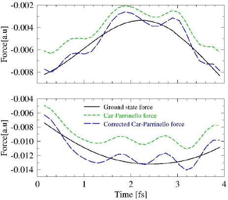
Figure 1: Some samples of force components on oxygen ions along a $4$ fs segment of CPMD trajectory $1$ ps after temperature has been adjusted using velocity rescaling. The Car-Parrinello force and the Car-Parrinello force once corrected with the best constant mass correction is compared to the ground state (Born-Oppenheimer) force, $F_{BO_{I}}$ at the same ionic positions.

Figure 1 demonstrates that, indeed, the difference between the Born-Oppenheimer and Car-Parrinello forces consists of both a systematic part $\Delta\mathbf{F}$, and an oscillatory part $\delta\mathbf{F}$. The systematic part appears to be mostly corrected by the application of mass corrections to the ions. The forces in figure 1 are those from a Car-Parrinello simulation in which velocity rescaling was employed for $0.5$ ps to bring the temperature from $T\sim 120K$ to $T\sim 220$ K. The velocities of the ions were adjusted only $4$ times, in total, during this $0.5$ ps . The system was then equilibrated for one picosecond after which the forces were examined along the $4$ fs segment of trajectory and compared to the forces at the same ionic positions, but with the orbitals in their ground state, i.e. the Born-Oppenheimer forces $\mathbf{F}_{BO_{I}}$. The amplitude of the oscillations, $\delta\mathbf{F}$, in figure 1 appears worryingly large. It will be shown in sections IV and VI, however, that if care is taken to ensure that the velocities of the ions are not changed discontinuously, the large amplitude of these oscillations disappears and the contribution of $\delta\mathbf{F}$ to the instantaneous error in the Car-Parrinello force can be neglected. At higher temperatures, however, large amplitude oscillations may always be present, as was the case in simulations of MgO in reference us, .

In section VI, the systematic part of the error $\Delta\mathbf{F}$, will be examined. It has been assumed in the pastkuo that $\Delta\mathbf{F}\approx\Delta\mathbf{F}^{m}$ and that $\Delta\mathbf{F}^{r}$ can be neglected. Therefore, in section VI, the validity of this assumption will be investigated. The degree to which $\Delta\mathbf{F}$ can be eliminated by applying mass corrections to the ions will be tested. In other words, the magnitude of $\Delta\mathbf{F}^{r}$, which has the potential to alter thermodynamic properties and for which no correction yet exists, will be examined.

IV Simulation Details

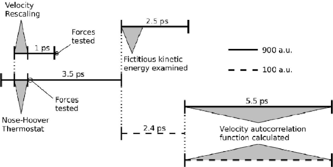
Figure 2: A schematic illustrating the sequence of Car-Parrinello molecular dynamics simulations that were performed.

In the CPMD simulations of D₂O reported here norm-conserving pseudopotentials have been used to describe oxygentrouillier_martins and deuteriumgygi and the valence electronic orbitals were expanded in plane waves with a maximum energy of 70 Rydberg. Simulations were performed on a $24\times 24\times 12$ a.u. simulation box containing $32$ D₂O molecules. Only the $\Gamma-$point was used to sample the Brillouin zone. A gradient-corrected functional was used to treat the effects of exchange and correlationblyp . In a preliminary CPMD simulation of liquid water mass corrections of $\Delta M_{O}=6.77\mu$ a.u. and $\Delta M_{D}=0.213\mu$ a.u. , were found for the oxygen and deuterium ions, respectively. These mass corrections were found by calculating the ground state forces at selected points along a trajectory and by minimizing the error in the CPMD forces relative to these ground state forces. These mass corrections were then used in all of the CPMD simulations of ice reported here by reducing the values of the ionic masses used in calculating the acceleration from Newton’s equation of motion i.e.

$$\ddot{R}_{I}^{\alpha}=-\frac{1}{\textrm{M}_{I}-\Delta\textrm{M}_{I}}\frac{\partial E[\{\psi_{i}\},\{\mathbf{R}_{I}\}]}{\partial R_{I}^{\alpha}}$$ (20)

The values of the fictitious mass used in the simulations reported here were $900$ a.u. and, for comparison, $100$ a.u. The equations of motion for electrons and ions were integrated using a molecular dynamics time step of $6$ a.u. for the $\mu=900$ a.u. simulations and $2$ a.u. for the $\mu=100$ a.u. simulations. No mass preconditioning scheme was used in any of the simulations reported here.

Much care has been taken to minimize errors in the simulations reported here. For example, as pointed out by Remler and Maddenremler , and discussed in section III.2 it is important that the velocities of the ions are not changed discontinuously as this can give a sudden kick to the electronic orbitals that results in large-amplitude ultra high frequency oscillations of the orbitals around their equilibria. Great care has therefore been taken to eliminate this source of error from the simulations reported here with the result (evident in figures 7 and 8 of section VI) that instantaneous errors in the forces due to ultra high frequency oscillations of the orbitals (i.e. $\delta\mathbf{F}$ ) are small enough relative to the systematic errors of equation 17 that they may safely be neglected.

The input coordinates for the CPMD were obtained by performing a very long molecular dynamics simulation of ice at low temperature ($\sim 100$ K ) using an ab initio parametrized polarizable atomistic potential of the same form as that constructed for silica in reference us_silica, . This potential does not provide a very realistic description of water but it was deemed preferable to using randomized initial coordinates. From these initial conditions a sequence of CPMD simulations were performed as shown schematically in figure 2. CPMD simulations were begun with the electrons in their ground state and the ions at zero velocity. A fictitious mass of $\mu=900$ a.u was used and therefore the ionic masses of oxygen and deuterium were rescaled to $M_{O}-\Delta M_{O}=12.659$ a.m.u and $M_{D}-\Delta M_{D}=1.895$ a.m.u, respectively and temperature was calculated using the true ionic masses of $M_{O}=16$ a.m.u and $M_{D}=2$ a.m.u. After half a picosecond of simulation in the microcanonical ensemble, the ions were at a temperature of $120$ K. At this point two separate continuations of the simulation were performed. The first continuation was performed in order to demonstrate the different contributions to the error in the forces on the ions and the effect of velocity rescaling on these forces, and has been discussed in section III.2. In the second continuation, a Nosé-Hoover thermostatnose was attached to the ions and the temperature was smoothly increased to approximately $250$ K during a further half picosecond of simulation. The system was then equilibrated without a thermostat for $3.5$ picoseconds. As shown in figure 3 the temperatures of the subsystems of oxygen and deuterium ions were calculated and compared with and without the use of the corrections to the masses of the ions in the definition of temperature. As can be seen, when mass corrections are used the oxygen and deuterium subsystems are at different temperatures indicating that the system is not well equilibrated.

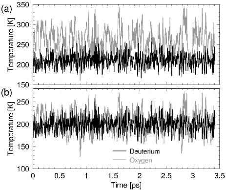
Figure 3: The temperatures of the oxygen and deuterium subsystems during the $3.5$ ps equilibration simulation with $\mu=900$ a.u. In (a) the temperatures have been calculated using masses for the ions that have been corrected to account for the extra inertia due to the weight of the Car-Parrinello orbitals (in this case $16$ a.m.u and $2$ a.m.u. due to the a priori rescaling of the masses). The oxygen and deuterium subsystems appear to be out of thermal equilibrium. In (b) the temperatures have been calculated in the standard way using the bare ionic masses ($12.659$ a.m.u and $1.895$ a.m.u). The oxygen and deuterium subsystems appear perfectly equilibrated.

If mass corrections are not used, the system appears perfectly equilibrated. At this point, the simulation was again continued in two separate simulations. In one of these simulations the value of $\mu=900$ a.u. was used as before. In another simulation the fictitious mass was changed to $\mu=100$ a.u. The rescaled masses of the ions in the simulation with $\mu=100$ a.u. were $15.629$ a.m.u. and $1.988$ a.m.u. If the rigid-ion approximation was perfectly applicable the fact that the ionic masses have been rescaled a priori would mean that the two simulations with different values of $\mu$ should have identical dynamic and thermodynamic behaviour.

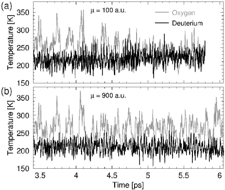
Figure 4: The temperatures of the oxygen and deuterium subsystems calculated using the corrected ionic masses ($M+\Delta M$) in the two continuations of the simulation shown in figure 3. In (a) a fictitious mass of $100$ a.u. has been used and thermal equilibration between the subsystems is observed. In (b) a fictitious mass of $900$ a.u. is used and the subsystems remain out of thermal equilibrium.

It was found (figure 4) that after more than a further $2.5$ ps the simulation with $\mu=900$ a.u. still showed no sign of thermalization according to the mass-corrected definition of temperature. However, the simulation with $\mu=100$ a.u. equilibrated quickly and the subsystems were at the same temperature after $1.5-2$ ps (figure  4). In order to compare the phonon spectra of ice using these two different values of $\mu$ for reasonably well equilibrated simulations at the same temperature it was decided to continue both simulations from the end of this initial $2.4$ ps run with $\mu=100$ a.u. For both $\mu=100$ a.u. and $\mu=900$ a.u., a further $5.5$ ps of simulation were carried out during which time the oxygen and deuterium subsystems remained at the same (mass-corrected) temperature in both simulations. For both values of $\mu$, the velocity autocorrelation function was calculated on a time domain of $1.45$ ps by averaging over this final $5.5$ ps of simulation. These velocity autocorrelation functions were then fourier transformed to obtain the phonon power spectra.

The reason for the inability of the $\mu=900$ a.u. simulations to thermalize during the first $7$ ps of simulation remains unclear. By using the dressed ionic masses in the calculation of temperature we are implicitly assuming that orbitals move rigidly with the ions and are unperturbed by their environment. In a condensed system this is an approximation and deviations from the rigid-ion limit always occur. In the opposite limit to the rigid-ion approximation, i.e. in the limit of very weak orbital-ion coupling, the temperature of the ions should be calculated with the bare ionic masses. For systems that are not perfectly ionic, therefore, the correct definition of temperature is unclear. While the results of section VI suggest that a constant mass correction for the ions is not perfectly appropriate for D₂O, the results of section V suggest that the rigid-ion approximation does a remarkably good job of estimating the fictitious kinetic energy of the orbitals. In addition, the fact that during the final $5.5$ ps of simulation the oxygen and deuterium subsystems remained at the same mass-corrected temperature suggests that it is appropriate to calculated temperature using rescaled masses.

The fact that reducing the value of $\mu$ appeared to facilitate thermalization may indicate that the thermalization problem was an artifact of the fictitious mass $\mu$, however, further work is required to clarify this issue.

V The time scale of orbital motion

A common view of CPMD is that, if a large enough gap exists between the energies of the occupied and unoccupied electronic states, the electronic orbitals move on time scales that are much faster than typical ionic time scales. For example, it has been suggested that the motion of the orbitals in CPMD can be approximately described as a superposition of oscillations whose frequencies are given by $\omega_{ij}=(\frac{2(\epsilon_{j}-\epsilon_{i})}{\mu})^{1/2}$, where $\epsilon_{i}$ and $\epsilon_{j}$ are the Kohn-Sham energy eigenvalues of occupied and unoccupied electronic states, respectivelymarx ; grossman ; caryip . In a system with a substantial energy gap between occupied and unoccupied states, all these frequencies are very high compared to typical ionic frequencies. In this view of CPMD the lowest vibrational frequency present in the orbital subsystem is determined by the size of the energy gap and the fictitious mass. However, it should be clear from the work of Pastore et al. and sections  II and  III of the present work that, if the orbitals are to remain close to the ground state and the ions are moving, their motion must contain an ionic time scale component. Here it is shown that, in fact, it makes the dominant contribution to the total orbital kinetic energy. The slow orbital motion results from the coupling between ions and the orbitals and it is precisely this coupling that leads to a systematic departure of the average forces in CPMD from the ground state forces.

If the rigid ion approximation holds perfectly, then the part of the kinetic energy of the orbitals due to the evolution of the electronic ground state can be obtained simply from the mass corrections and the velocities of the ions, i.e.

$$\sum_{i}\mu\langle\dot{\psi}_{i}|\dot{\psi}_{i}\rangle=\frac{1}{2}\sum_{I\epsilon O}\Delta M_{O}\dot{R}_{I}^{\alpha}\dot{R}_{I}^{\alpha}+\frac{1}{2}\sum_{I\epsilon D}\Delta M_{D}\dot{R}_{I}^{\alpha}\dot{R}_{I}^{\alpha}$$ (21)

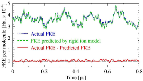
Figure 5: The fictitious kinetic energy (FKE) of the electronic orbitals as a function of time compared to the FKE predicted by assuming that orbitals are inert and rigidly follow the ions. The close agreement between the curves verifies that orbital motion occurs primarily on ionic time scales and that the contribution of the ultra-high frequency oscillations of the orbitals about their instantaneous equilibria to the total FKE is tiny by comparison.

In figure  5 the fictitious kinetic energy (FKE) as predicted by the rigid ion model in equation  21 is compared to the FKE that is extracted from the CPMD simulation. The difference between them is also plotted and this is made up both of ultra high frequency oscillations of the orbitals about their instantaneous equilibria and the part of the ionic time scale evolution of the ground state that cannot be described within the rigid ion approximation. The very close agreement between the predicted FKE and the actual FKE demonstrates clearly that electronic orbitals move on ionic time scales and, furthermore, that this slow motion accounts for almost all of their fictitious kinetic energy. This also demonstrates that the lowest vibrational frequencies of the orbital subsystem are almostalmost independent of $\mu$ and are simply given by the lowest vibrational frequencies of the ionic subsystem. Some previous simulations have calculated the orbital vibrational power spectrum by fourier transforming the orbital velocity autocorrelation function and have not detected such low frequenciespastore ; grossman . However, in these simulations the orbital vibrations were analysed while the ions were kept stationary and therefore the contribution to the orbital motion from the evolution of the electronic ground state was not present. In reference herbert, Herbert and Head-Gordon have analysed the orbital vibrations during ion dynamics, and figure 7 of that paper clearly shows a contribution to the orbital frequency spectrum that has a low (ionic) frequency and that appears almost independent of the fictitious mass.

VI Forces

The goal of first principles molecular dynamics is to make a direct connection between an accurate description of the electrons and an accurate calculation of the physical property of interest. It is important to know that a calculated physical property that agrees well with experiment does so because the trajectory is realistic due to good forces calculated from a good treatment of the electronic structure. When there is a microscopic basis for agreement with experiment the method can be applied with some confidence to situations or to properties for which experimental data is unavailable. This point is stressed because agreement with experiment in molecular dynamics simulations can often occur due to a cancellation of errors. This has been observed both in first principles simulationsgrossman and in simulations using empirical potentials where potentials that agree with experiment on many propertiesbks have been found to provide a very poor microscopic description of the interatomic forcesus_silica .

It is obvious, therefore, that in order to proceed without recourse to empiricism or a posteriori experimental verification one should be able to depend on the accuracy of the computed forces. What is much less obvious is how one should judge the accuracy of forces. One way of quantifying the average magnitude of the departure of a set of forces $\{F_{I}\}$ from some reference forces $\{F^{\text{ref}}_{I}\}$ is by computing the percentage root-mean-squared difference between the two sets of forces relative to the root-mean-squared force component, i.e. :

$$\Delta_{rms}=100\times\frac{\sqrt{\sum_{I,\nu}\|F_{I}-F^{\text{ref}}_{I}\|^{2}}}{\sqrt{\sum_{I,\nu}\|F^{\text{ref}}_{I}\|^{2}}}$$ (22)

where the sum $\sum_{I,\nu}$ is over a large number of ions $I$ and over a large number of points $\nu$ along the molecular dynamics trajectory. In general, this is an extremely crude measure of the departure of the forces from the reference forces, however there is frequently no alternative to using it. A number of classical potentials have been parametrized by minimizing this quantity while using ground state density functional theory forces as the reference. It has been found that, for some simple oxides, values as low as $\Delta_{rms}=5-20\%$ can be achieved and that, as long as $\Delta_{rms}$ is sufficiently small (i.e. $<20\%$ ), the accuracy of these force fields for many experimental quantities is well correlated with its valueus_silica ; us_mgo . Although it is crude and unsatisfactory, in the absence of an alternative quantitative general measure of the quality of forces in the presence of errors of unknown consequence, this quantity is used in the present work.

In this section the forces on the ions in the CPMD simulations of ice are inspected along a segment of the trajectory. After approximately $1$ ps of simulation the ground state forces were calculated along a $21$ fs segment of the CPMD trajectory. These ground state forces were then used as the reference forces for calculating the root-mean-squared (r.m.s) relative error in the CPMD forces according to equation 22 both before and after they had been corrected using the rigid-ion mass correction. In other words (using the notation introduced in section III.2 and assuming that $\delta F_{I}^{\alpha}$ is negligible) the r.m.s. values of $\Delta F_{I}^{\alpha}$ and $\Delta F_{I}^{r\;\alpha}$ relative to the r.m.s. value of $F_{BO_{I}}^{\alpha}$ were computed. Before mass corrections were applied it was found that, for oxygen ions, $\Delta_{r.m.s}$ amounted to $21.8\%$. In other words, the r.m.s. error in the forces on the oxygen ions was $21.8\%$ of the r.m.s. oxygen ion force component. For the deuterons $\Delta_{r.m.s}$ was $5.5\%$. The force on each atom is dominated by intra-molecular interactions which are relatively constant (in the reference frame of the molecule) at room temperature and therefore are generally of much less interest to simulators than the inter-molecular interactions. For this reason, the most important quantity to examine is the net force on each water molecule. It was found that $\Delta_{r.m.s}$ for the net forces on the water molecules was $44.7\%$. The values of the mass corrections for the oxygen and deuterium ions were varied so as to minimize $\Delta_{r.m.s}$ for the corrected forces. It was found that by applying mass corrections of $\Delta M_{O}=6.91\mu=3.41$ a.m.u and $\Delta M_{D}=0.215\mu=0.11$ a.m.u the errors could be reduced substantially to $5.3\%$ for oxygen, $1.4\%$ for deuterium and $12.4\%$ for the water molecules. These mass corrections are very close to those that were applied a priori based on preliminary tests of liquid water but in fact it was found that, for oxygen, a wide range of values of $\Delta M_{O}$ gave very similar values for the average error. The value of $\Delta_{r.m.s.}$ for the corrected oxygen and water molecule forces is plotted in figure 6 as a function of the mass correction for the oxygen ion. $\Delta_{r.m.s.}$ is found to be reasonably insensitive to the mass correction near the average optimal value because the optimal mass correction varied from atom to atom or, for a given atom, it varied in time. By changing the value of $\Delta M_{O}$ one improved the agreement of some of the forces with the ground state forces and disimproved others. It was also found that the mass correction that gave best agreement between ground state and corrected CPMD forces on a given atom was different, in general, for the different Cartesian components. In other words, the effective masses of the ions in this simulation were time-varying tensor quantities as is to be expected from equation 17.

Figure 6: The r.m.s relative error $\Delta_{r.m.s}$ in the mass-corrected forces on the oxygen ions (full line) and on the D₂O molecules on the sample segment of the CPMD trajectory as a function of the magnitude of the mass correction. $\mu=900$ a.u. in this simulation.

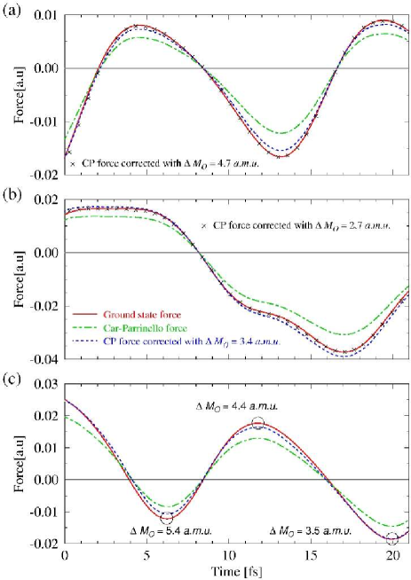
Figure 7: Some samples of force components on oxygen ions along a $21$ fs segment of CPMD trajectory. The Car-Parrinello force (green) and the Car-Parrinello force once corrected with the best constant mass correction (blue) is compared to the ground state force at the same ionic positions. Also plotted in (a) and (b) are the Car-Parrinello forces once corrected using the optimal mass correction for that ion along this particular segment of trajectory. In (c) the optimal mass correction at three points along the trajectory are indicated.

In figure 7 some sample force components on oxygen ions are shown to illustrate this fact. Figure 7 (a) and figure 7 (b) are examples of oxygen ions which, over this segment of trajectory, have different effective masses. Fig. 7 (c) is an example of an oxygen ion force component for which the optimal mass correction varies considerably over this short length of trajectory. The large oscillations of the Car-Parrinello forces of period $\sim 1$ fs that were visible in figure 1 are completely absent in figure 7, demonstrating that the contribution, $\delta\mathbf{F}$, of the ultra high frequency oscillations of the orbitals to the force is negligible due to the ions having been accelerated continuously throughout this simulation.

In figure 8 some sample force components on molecules are shown and compared to the ground state force and the force once corrected using the average optimal mass corrections.

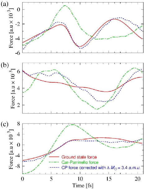
Figure 8: Some samples of force components on D₂O molecules along a $21$ fs segment of CPMD trajectory. The Car-Parrinello force (green) and the Car-Parrinello force once corrected with the best constant mass corrections (blue) is compared to the ground state force at the same ionic positions.

It is clear from Fig. 7 and Fig. 8 that the errors in CPMD forces due to the fictitious mass can not simply be described in terms of a constant correction to the masses of the ions. In other words, the $\{\Delta F^{r\;\alpha}_{I}\}$ are quite large.

To get some perspective on the level of errors in the forces, these errors are compared in magnitude to those at varying levels of convergence of the Kohn-Sham orbitals to their ground state during a minimization using the method of direct inversion in the iterative subspace (DIIS)diis . Fifteen equally-spaced atomic ‘snapshot’ configurations were extracted from the final $5.5$ picosecond production run with $\mu=900$ a.u. and, starting with random wavefunctions, the Kohn-Sham energy was minimized. Convergence of this minimization was taken to mean that the difference in energy between successive electronic iterations $\delta_{scf}$ had fallen lower than $10^{-13}$ a.u./atom. For each snapshot configuration all iterations for which $\delta_{scf}>10^{-3}$ a.u./atom were discarded. At all other iterations the percentage r.m.s errors in the forces $\Delta_{rms}$ relative to the fully converged forces were calculated.

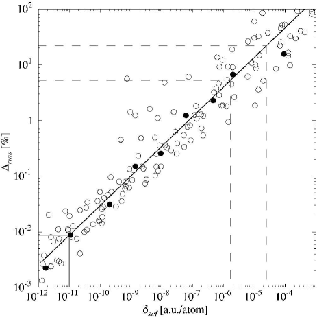
Figure 9: The r.m.s relative error $\Delta_{r.m.s}$ in the forces as a function of the degree of convergence $\delta_{s.c.f}$ of the total energy during minimizations to the ground state with DIIS for $15$ ’snapshot’ atomic configurations extracted from the CPMD simulations. Each circle corresponds to a single self-consistency step in the minimization of the wavefunctions for a single snapshot. The filled circles are the data from one full representative DIIS minimization and are included to illustrate the convergence characteristics for each snapshot. The dashed lines indicate the value of $\Delta_{r.m.s.}$ from the mass corrected and uncorrected forces in the CPMD simulations and the level of convergence of the total energy that this would correspond to. The grey line indicates the level of convergence that is typically used in BOMD simulations of water ( $\delta_{s.c.f}=10^{-11}$ a.u./atom ) and the value of $\Delta_{r.m.s.}$ that this corresponds to.

A line was then fit to the dependence of $\log_{10}\Delta_{rms}$ on $\log_{10}\delta_{scf}$. This was done separately for the forces on the oxygen ions, the deuterons and the water molecules. The comparison with the errors in CPMD is quantitatively very similar in each case and therefore only the results for the oxygen ions are plotted in figure 9. Very similar results were also found when electronic minimization was performed using a conjugate-gradients technique and therefore it is assumed that, for the purpose of the present discussion, the dependence of $\Delta_{r.m.s.}$ on $\delta_{s.c.f}$ could be assumed to be reasonably independent of the route taken to the electronic ground state. For comparison, the values of $\Delta_{rms}$ for the forces from the CPMD simulations both before and after the application of the rigid-ion mass corrections are also shown in this figure 9. The results suggest that, for the mass corrected (uncorrected) forces, the degree of convergence required at each time step of a BOMD simulation in order to achieve an average error in the forces $\Delta_{r.m.s.}$ of the same magnitude is around $\delta_{s.c.f}=10^{-5}$ a.u./atom ($=10^{-4}$ a.u./atom ). This is many orders of magnitude larger than the level of convergence that is generally used for waterasthagiri_pre ; schwegler ; kuo ; vandevondele . For example, in reference kuo, BOMD simulations were performed with a convergence of the energy at each step of $\delta_{s.c.f}=10^{-11}$ a.u./atom. It was reported that this simulation was about a factor of $4$ more expensive than a CPMD simulation that used a time step of $4$ a.u. As illustrated in figure 9 the errors in the forces are about three orders of magnitude smaller than those in the CPMD simulation when $\delta_{s.c.f}=10^{-11}$ a.u./atomforce_comparison . A fair comparison between BOMD and CPMD should consider their relative efficiencies at the same level of accuracy or their relative accuracies at the same level of efficiency. In general, this comparison depends on the system under consideration and the level of accuracy (or efficiency) required. No attempt will be made here to study this question in detail. However, it is illuminating briefly to consider the relative efficiencies of BOMD and CPMD at the level of accuracy of a CPMD simulation with $\mu=900$ a.u., and at the level of accuracy of a BOMD simulations with $\delta_{s.c.f}=10^{-11}$ a.u./atom .

It is assumed here that the efficiency of BOMD for ice is similar to that of water. Drawing on the results of Kuo et al., it is therefore assumed that a BOMD simulation with $\delta_{s.c.f}=10^{-11}$ is approximately three times slower than a CPMD simulation with $\mu=900$ a.u. and $\Delta t=6$ a.u. Assuming that errors in the forces scale linearly with $\mu$, $\Delta_{r.m.s.}$ for the CPMD simulation can be reduced to the level of the highly converged BOMD simulation by reducing $\mu$ by about three orders of magnitudeforce_comparison . The time step required to integrate the equations of motion for the orbitals scales with the square-root of the fictitious mass, and therefore this reduction of $\mu$ requires a reduction of the time step (and therefore the speed of the simulation) by a factor of about $30$. What this means is that, at this level of accuracy, BOMD is roughly an order of magnitude faster than CPMD.

If a much lower accuracy is sufficient, such as the level of accuracy in a CPMD simulation with $\mu=900$ a.u., then a comparison with a BOMD simulation using a value of $\delta_{s.c.f}$ that is five or six orders of magnitude larger is sufficient. At this level of convergence, the BOMD simulation of Kuo et al. would be faster, but because $\delta_{scf}$ typically reduces by an order of magnitude with each one or two electronic iterations, the speed up may not be very great. It would depend on the average rate of convergence of the orbitals to the ground state and on the quality of the extrapolation of the orbitals from previous time steps. It seems likely that the speeds of CPMD and BOMD simulations would be much closer in this case. However, a BOMD simulation at this level of accuracy would suffer from discontinuous forces - a problem that is not present in CPMD.

More detailed comparisons between CPMD and BOMD are clearly required. The point of the present discussion is simply that the accuracy (as judged by the quantity $\Delta_{rms}$) of a reasonably well-converged BOMD simulation far exceeds that of a CPMD simulation using standard values (a few hundred atomic units)large_mass of the fictitious mass. The argument that CPMD is more efficient than BOMDkuo is frequently based on comparisons in which BOMD is held to a higher standard of accuracy than CPMD.

VII Phonon power spectrum

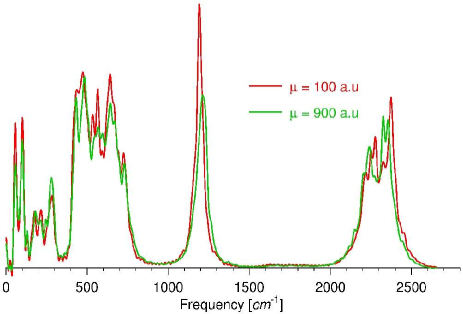
Figure 10: The mass-corrected phonon power spectra for simulations with $\mu=100$ a.u. and $\mu=900$ a.u.

As described in section  IV, the phonon power spectra have been calculated for the simulations with $\mu=100$ a.u. and $\mu=900$ a.u. The results are plotted in figure 10. Different rescaled masses have been used in these two simulations and so the coincidence of the main peaks in these power spectra clearly vindicates the use of corrections to the masses of the ions. For MgO, it has already been demonstrated that the power spectrum is strongly altered by the fictitious mass if mass corrections are not appliedus . In the present work only the corrected power spectra are presented, but it should be clear that, if the masses of the ions had not been rescaled a priori, the power spectrum of the simulation with $\mu=900$ a.u., in particular, would have been very different. Overall, the agreement between the two power spectra is reasonably good despite the fact that, as discussed in section  VI, the masses of the oxygen ions vary considerably during the dynamics and that the mass correction that was applied was simply a uniform constant correction to account for the average value of the extra inertia of the ions due to the fictitious mass. It may be that many time- or space-averaged properties are insensitive to $\mu$ as long as average constant mass corrections are applied to the ions. For example, the work of Grossman, Schwegler et al.grossman ; schwegler suggests that once adiabatic decoupling is achieved, the pair-distribution function of water is not very sensitive to the value of $\mu$footnote .

VIII Discussion

In the present work and in reference us, it has been shown that the inertia associated with the Kohn-Sham orbitals in CPMD can affect the motion of the ions. There are substantial differences between the CPMD forces and the ground state forces at the same ionic positions. Reference us, focussed on two materials that exhibit extreme behaviour. Crystalline MgO under pressure is an almost perfectly ionic material with a high quantum kinetic energy associated with valence electrons that are strongly bound to the oxygen ions. The $\mu$-dependent error for MgO is therefore very large but can almost perfectly be corrected by applying a constant mass correction to the ions. Silicon, on the other hand, is a material in which valence electrons are delocalized and have a small quantum kinetic energy. $\mu$-dependent errors for silicon are therefore extremely small.

Here the focus has been on D₂O - an important system in which valence electrons possess a large amount of quantum kinetic energy, but which is not perfectly ionic. It is demonstrated that $\mu$-dependent errors are large, and while applying a constant mass correction to the ions improves the forces considerably, systematic errors ($\Delta F^{r}$ ) remain that are very large compared to the errors that would be present in a reasonably well-converged BOMD simulation. These errors are highlighted in order to underline the importance of caution when applying CPMD to situations in which substantial rearrangements of the electronic orbitals are likely to occur. The non-rigid-ion part of the errors, $\Delta F^{r}$, observed for crystalline D₂O are likely to be less serious than those in liquid water, for example, where deviations of the electronic orbitals from their average structure are likely to be larger. Furthermore, in studies of chemical reactions and phase transitions deviations from rigid-ion behavior are likely to be more serious and it may not be safe to assume that dynamics and thermodynamics can be corrected simply by using mass corrections for the ions. In such situations it would appear safer to use a small value of $\mu$ or to use BOMD.

In the past, the quality of a CPMD simulation has sometimes been judged according to the degree of conservation of energy and the degree to which the adiabatic-decoupling condition is maintainedkuo . In the present work it has been emphasized that adiabatic decouping is not a decoupling of the ions from the orbitals but only a decoupling of the ultra high-frequency part of the orbital motion from the lower-frequency modes of the coupled orbital-ion system. Perfect energy conservation and perfect adiabatic decoupling have both been maintained in the simulations of D₂O presented here, and yet the accuracy of the computed forces is quite poor.

Comparisons between BOMD and CPMD in this work have relied on calculating the average magnitude of systematic errors, $\Delta F$, (i.e. errors that do not average out on short time scales) in the forces on the ions. While there is no obvious alternative to using this quantity, and while the disparity in the magnitude of the errors between CPMD and BOMD appears largeforce_comparison , it should be borne in mind that this is an extremely crude measure of the accuracy of a simulation. The effects of the errors in the forces in CPMD and BOMD are likely to be different. Although an analytic expression for the error in the forces in the case of CPMD is given by equation 17 the effect on thermodynamic properties of the part of this error that does not reduce to a mass correction, i.e. $\Delta\bf{F}^{r}$, is not obvious.

In BOMD, the errors in the forces lead to a systematic drift in the total energy due to a systematic bias in the wavefunctions arising from their extrapolation from previous time stepspulay . This energy drift can be a very useful judge of the accuracy of a simulation, however, a consequence of this is that there is also a drift in the temperature that, for long simulations, needs to be counter-balanced through the use of a thermostat for the ions. Apart from this obvious change in the temperature, the effects of errors in the BOMD forces on thermodynamic properties is unknown, in general. Recent work by Pulay and Fogarasi has suggested counteracting the energy drift by adding small corrections to the velocities of the ions at each time steppulay . This procedure might allow a BOMD simulation to be performed with a convergence criterion for the electronic structure that is less strict than commonly used criteria as it could be both faster and with smaller average errors in the forces than are present in CPMD. A disadvantage of performing poorly converged BOMD simulations is that the forces on the ions would be discontinuous in time, and the simulations would not be time-reversible. In conservative CPMD simulations forces are always continuous and simulations are always time-reversible regardless of the accuracy of the forces.

In CPMD the average kinetic energy of the ions can remain approximately constant throughout a simulation. In other words, while orbitals and ions are constantly exchanging energy and momentum in CPMD, if the adiabatic decoupling condition is maintained there is no systematic net transfer of energy between them. Ions both gain momentum from and lose momentum to the orbitals in CPMD and the physically meaningful total energy, which is the sum of the kinetic energy of the ions and the Kohn-Sham energy, fluctuates about a constant. The fluctuations in this energy are exactly mirrored by the fluctuations in the fictitious kinetic energy because their sum is conserved. Therefore, the accuracy of CPMD can, in principle, be judged by the fluctuations in the FKE although how this should be done in practice is less obvious. As can be seen from figure 5, because care was taken to avoid discontinuously accelerating the orbitals, only ionic-timescale fluctuations are visible in the FKE. When the rigid-ion contribution to the FKE is subtracted out, the FKE that remains is much smaller and with much smaller fluctuations, however, section VI shows that the average remaining error in the forces is still orders of magnitude larger than would be found in a reasonably well converged minimization of the orbitals to the electronic ground state. This is simply an illustration of the fact that small fluctuations in the energy (which varies only to second order in $\delta\psi$) can result in much larger fluctuations in the force (which varies to first order in $\delta\psi$ ). It also suggests that it may be worth examining the effect on forces rather than energies of the use of thermostats to control the FKEblochl_and_parrinello ; blochl2 .

Currently, ab initio molecular dynamics (AIMD) is hampered by two very important problems. The first of these is the limitations on the time scales and length scales that are accessible to simulations. This problem means that many properties and systems are currently beyond the reach of AIMD. For simulations that can be performed, this problem severely limits the precision with which thermodynamic properties are calculated. The second major problem is that the density functionals that are currently in use are not accurate enough for many applications, particularly in the study of chemical reactions where a high level of accuracy is required on the energetics, and in systems in which electron correlation plays a prominent role. Both of these problems will gradually be reduced by technological, algorithmic and theoretical innovations and therefore the relative importance of the kinds of errors described in the present work will increase.

It should be stressed that in the present work and in reference us, , apart from clear problems with vibrational properties due to increased ionic masses, and changes in the definition of temperature, thermal pressure, and other quantities that depend explicitly on the mass, no observable thermodynamic quantity has been demonstrated to deviate significantly from the value that would be obtained in a perfectly converged BOMD simulation. It may be that further testing will reveal that, in practice, many properties are rather insensitive to $\mu$ as long as constant mass corrections are applied to the ions. Clearly, given the magnitude of the errors demonstrated in the present work, and the lack of an obvious theoretical justification for CPMD when $\mu$ is large and the electronic structure deviates significantly from the rigid-ion limit, further testing is necessary.

IX Conclusions

What has been demonstrated in the present work is that there are problems with some of the arguments that have been used in the past to theoretically justify CPMD. The forces in CPMD differ from the ground state forces even when averaged on a femtosecond time scale and even when constant mass corrections have been applied to the ions. For commonly used values of the fictitious mass, $\mu$, the magnitude of these errors in the forces is large compared to the errors that would generally be tolerated in a BOMD simulation. How the errors in CPMD impact on thermodynamic properties is unknown. The errors can systematically be reduced by reducing the value of $\mu$.

- (1) R. Car and M. Parrinello, Phys. Rev. Lett. 55, 2471 (1985).
- (2) W. Kohn and L. Sham, Phys. Rev. 140, A1133 (1965).
- (3) P. Hohenberg and W. Kohn, Phys. Rev. 136, B864 (1964).
- (4) P. Tangney and S. Scandolo, J. Chem. Phys. 116 , 14 (2002).
- (5) J. C. Grossman, E. Schwegler, E. W. Draeger, F. Gygi, and G. Galli, J. Chem. Phys. 120, 300 (2004).
- (6) E. Schwegler, J. C. Grossman, F. Gygi, and G. Galli, J. Chem. Phys. 121, 5400 (2004).
- (7) This orthogonality condition is more conventionally included explicitly in the Lagrangian as a holonomic constraint, however, for the purposes of clarity and convenience of notation it is made implicit in the functional derivatives throughout this paper.
- (8) M. C. Payne, J. D. Joannopoulos, D. C. Allan, M. P. Teter and D. H. Vanderbilt, Phys. Rev. Lett. , 56, 2656 (1986).
- (9) D. Marx and J. Hütter in Modern Methods and Algorithms of Computational Chemistry; Grotendorst, J., Ed.; John von Neumann Institute for Computing: J lich, 2000; Vol. 1, p 329.
- (10) I-Feng W. Kuo, C. J. Mundy, M. J. McGrath, J. I. Siepmann, J. VandeVondele, M. Sprik, J. Hütter, B. Chen, M. L. Klein, F. Mohamed, M. Krack, M. Parrinello, J. Phys. Chem. B 108, 12990 (2004).
- (11) R. Car, F. de Angelis, P. Giannozzi, and N. Marzari, in Handbook of Materials Modeling, Vol. 1: “Methods and Models”, Editor S. Yip, Volume Editors: E. Kaxiras, N. Marzari, and B. Trout (Springer, 2005).
- (12) G. Pastore, E. Smargiassi and F. Buda, Phys. Rev. A44, 6334 (1991)
- (13) J. VandeVondele and A. De Vita Phys. Rev. B 60, 13241 (1999).
- (14) P. E. Blöchl and M. Parrinello, Phys. Rev. B 45, 9413 (1992).
- (15) P. E. Blöchl Phys. Rev. B65, 104303 (2002).
- (16) P. E. Blöchl, Phys. Rev. B50 17953 (1994).
- (17) See, for example K. Laasonen, M. Sprik, M. Parrinello, and R. Car, J. Chem. Phys. 99, 9080 (1993); M. Sprik, J. Hütter, and M. Parrinello, J. Chem. Phys. 105, 1142 (1996); P. L. Silvestrelli and M. Parrinello, J. Chem. Phys. 111, 3572 (1999).
- (18) See, for example : M. J. Field, Chem. Phys. Lett. 172 83 (1990) ; B. Hartke and E. A. Carter, Chem. Phys. Lett. 189 358 (1992) ; D. A. Gibson and E. A. Carter, Chem. Phys. Lett. 271 266 (1997) ; Z. H. Liu, L. E. Carter, and E. A. Carter, J. Phys. Chem. 99 4355 (1995);
- (19) M. Sprik and M. L. Klein J. Chem. Phys. 89 7556 (1988)
- (20) M. Sprik J. Phys. Chem. 95 2283 (1991)
- (21) S. W. Rick, S. J. Stuart, and B. J. Berne J. Chem. Phys. 101 6141 (1994).
- (22) J. Genzer and J. Kolafa J. Mol. Liq. 109 63 (2004).
- (23) R. Car in Quantum Theory of Real Materials, Editors J.R. Chelikowsky and S.G. Louie, (Kluwer Academic, Boston, 1996), pp. 251-259.
- (24) P. Tangney, Ph.D Thesis, SISSA, Trieste (2002), available to download at : http://www.sissa.it/cm/phd.php.
- (25) Note that the sign of the expression for in equation 17 differs from that of reference us, while the sign of the mass correction of equation 18 is the same in both cases. This is due to two separate sign errors that occur in equations 8 and 23 of reference us, . These errors are repeated in reference thesis, .
- (26) D. J. Tobias, G. J. Martyna, and M. L. Klein, J. Phys. Chem. 97 12959 (1993).
- (27) N. Trouiller and J. L. Martins, Phys. Rev. B 43, 1993 (1991)
- (28) F. Gygi, Phys. Rev B 48, 11692 (1993).
- (29) D. Vanderbilt, Phys. Rev. B 41, 7892 (1990).
- (30) A. D. Becke, Phys. Rev. A38, 3098 (1988); C. Lee, W. Yang, and R. C. Parr, Phys. Rev. B37 , 785 (1988).
- (31) D. K. Remler and P. A. Madden, Mol. Phys. 70, 921 (1990).
- (32) P. Tangney and S. Scandolo, J. Chem. Phys. 117, 8898 (2002).
- (33) S. Nosé, Mol. Phys. 52, 255 (1984); S. Nosé, J. Chem. Phys. 81, 511 (1984); G. H. Hoover, Phys. Rev. A 31, 1695 (1985).
- (34) There is an indirect dependence of the lowest frequency of the orbital subsystem through the dependence of the ionic frequencies on .
- (35) J. M. Herbert and M. Head-Gordon, J. Chem. Phys. 121, 11542 (2004).
- (36) B. W. H. van Beest, G. J. Kramer, R. A. van Santen, Phys. Rev. Lett. 64 , 1955 , (1990).
- (37) P. Tangney and S. Scandolo, J. Chem. Phys. 119, 9673 (2003).
- (38) P. Pulay, Chem. Phys. Lett. 73, 393 (1980); G. Kresse and J. Furthmuller, Phys. Rev. B 54, 11169 (1996).
- (39) D. Asthagiri, L. R. Pratt, and J. D. Kress Phys. Rev. E 68, 041505 (2003).
- (40) J. VandeVondele, F. Mohamed, M. Krack, J. Hütter, M. Sprik, and M. Parrinello, J. Chem. Phys. 121, 014515 (2005).
- (41) The average error in the forces for obtained from the straight line fit to the minimization results of Figure 6 is . This is approximately () times smaller than the error in the mass corrected (uncorrected) forces in the CPMD simulation with a.u.
- (42) I. Ivanov and M. L. Klein, J. Am. Chem. Soc. 127, 4010 (2005); J. Blumberger and M. Sprik, J. Phys. Chem. B 109, 6793 (2005); B. Kirchner and J. Hütter J. Chem. Phys. 121, 5133 (2004); S. Churakov, M. Iannuzzi, and M. Parrinello, J. Phys. Chem. B 108, 11567 (2004).
- (43) P. Pulay and G. Fogarasi, Chem. Phys. Lett. 386, 272 (2004).
- (44) Corrections to temperature as described in Ref. us, and in sections III and IV of the present work were not applied in references grossman, and schwegler, and this complicates the interpretation of their results, however, it seems unlikely that these temperature corrections are large enough to qualitatively alter their findings.