Long-Range Order and Interactions of Macroscopic Objects in Polar Liquids.

Abstract

We develop a phenomenological vector model of polar liquids capable to describe aqueous interactions of macroscopic bodies. It is shown that a strong, long-range and orientationally dependent interaction between macroscopic objects appears as a result of competition between short-range (hydrogen bonding) and the long-range dipole-dipole interactions of the solvent molecules. Spontaneous polarization of molecular dipoles next to a hydrophobic boundaries leads to formation of globally ordered network of hydrogen-bonded molecules with ferroelectric properties. The proposed vector model naturally describes topological excitations on the solute boundaries and can be used to explain the hydrogen bonds networks and order-disorder phase transitions in the hydration water layer.

I Introduction.

Interactions of macroscopic bodies in aqueous environments is a fundamentally important problem in physics, chemistry, structural biology and in silico drug design. The main theoretical difficulty arises both from strong long-range dipole-dipole interactions of molecular dipole moments and complicated nature of short-range interaction between water molecules. For practical purposes, e.g. calculation of binding free energy (inhibition constant) of a protein-ligand complex, protonation states predictions for biomacromolecules, physics of membranes etc, the ultimate way to quantitatively account for solvation effects is the Free Energy Perturbation method (FEP) based on a direct modelling of both the solute and the solvent molecules, molecular dynamics (MD). One of the main advantages of MD is a possibility to include the surrounding water molecules into the calculation directly (simulations with explicit water). In fact this is so far one of the most accurate ways to compute the solvation and the binding energies ModernMD . The limitation of the method comes together with its strength: to do it one should compute coordinates and velocities of very large number of atoms with time step $\tau_{S}\sim 10^{-15}s.$ To allow the aqueous environment to relax fully, the averaging needs to be performed on a sufficiently long time span to include at least the life-time of hydrogen bonds ($\sim 10^{-9}s$), and even the much larger relaxation and rearranging time of macroscopic water clusters (up to $\sim 10^{-6}s$, see discussion below). For modern computers it is possible to follow the evolution of macromolecules in water environment up to times $\sim 10^{-7}s$, which may not be sufficient to relax the surrounding water molecules in some situations. Although such calculations can be very accurate, realistic applications require enormous computational resources.

Polar liquids such as water are characterized by large values of static dielectric constants $\epsilon\gg 1$. That is why to a large extent solvation theory can be reduced to a macroscopic electrostatics with a solvent being modelled as a high-$\epsilon$ media and the solute treated as being emerged in a low-$\epsilon$ cavity. This approach dates back to early Born’s papers and can be very successful for quantitative predictions of solvation energies of small molecules or biomolecules interactions Karplus ; Onufriev . On other hand the interactions of sufficiently small neutral objects is dominated by hydrophobic effect, which according to Chandler ; Lum ; Wolde originates from short-range interactions of the solvent molecules. Density functional models Chandler ; Lum ; Wolde successfully explain the hydrophobic interactions on molecular scales, though inclusion of electrostatic interactions appears to be a difficult task. Moreover, understanding of a number of important observations revealed from MD simulations must require complete inclusion of long-range interactions and thus a more sophisticated approach. Among the examples are the arrangement of the water molecules dipole moments parallel to the hydrophobic surface MD1 ; MD2 ; MD3 , the vortex-like structures of molecular dipole moments networks and dipole-bridges near and between the solvated objects Higo .

In this Letter we introduce a continuous vector model of a polar liquid capable both the short- and the long-range features of a polar liquid in a single theoretical framework. The model can be applied to aqueous interactions of macroscopic bodies of various shapes and charges. It is shown that the competition between the short range (hydrogen bonding) and the long-range dipole-dipole interactions of the solvent molecules leads to appearance of strong, long range and orientationally dependent interactions between macroscopic objects. A polar liquid itself is characterized by a complicated fluctuating thermal state, ordered at sufficiently short scales within a single domain, and completely disordered at larger distances. This physical picture has far reaching consequences, especially at solvent-solute surfaces, where the ferroelectric film of solvent molecules is formed. With temperature increasing fluctuations of molecular dipole moments can lead to topological phase transitions depending on hydrophobic properties of the interface. We argue that the dynamics of macroscopic topological excitations on a surface of the liquid may be a physical picture behind the percolation transition of the hydrogen bonding network observed in MD simulations Oleinikova1 ; Oleinikova2 ; Oleinikova3 .

The manuscript is organized as follows. After the introduction in Section 2 we discuss the basic assumptions and formulate the vector model of polar liquids mathematically. In following Section we discuss the bulk properties and the correlation functions of the liquid within the model. The results of the discussion can be used to calculate various asymptotic forms of interactions between point-like and macroscopic bodies of different shapes and charged states in a solute. At last, in Section 4 we address the properties of hydration layers of molecular dipoles on macroscopic surfaces with the emphasis on topological properties of hydrogen bonds networks and possible phase transitions.

II The model.

Polar liquids are similar to ferroelectrics. Having this analogy in mind it is possible to develop a vector field theory in which the liquid is described by a local mean value of the molecular polarization vector

$$\mathbf{s}(\mathbf{r})=\langle\mathbf{d}\rangle/d_{0}$$ (1)

Here $d_{0}$ is the static dipole momentum of a single molecule, and the averaging of molecular dipole momentums $\mathbf{d}$ is performed over a small but macroscopic volume of the liquid containing macroscopic number of molecules. Mathematical structure of theory of ferroelectrics Ginzburg is analogous to the phenomenological Landau-Ginzburg theory for ferromagnetics, which deals with the average value of atomic magnetic moment. All essential properties of a polar liquid are the result of competition of two opposite effects, two types of interaction: the long-range electrostatics (dipole-dipole interaction) $\Omega_{dd}$ and the short-range intermolecular potential, $\Omega_{H}$, responsible for hydrogen bonds (H-bonds) formation. At room temperatures quantum-mechanical effects dominate in $\Omega_{H}$ . As for $\Omega_{dd}$ , it has pure classical nature. As the Earnshaw’s theorem says, the equilibrium state is impossible for the system of classical charges Sivukhin ; Stratton . It means that $\Omega_{dd}$ leads to chaotization of molecular dipole momenta orientations, and hence the ground state of a polar liquid is a disordered state at least on a large scale. At smaller distances however, the molecules tend to form maximal possible number of H-bonds, and thus the H-bond interactions order the molecular dipole moments.

Below we employ the following expression for the free energy of the liquid:

$$\Omega(\mathbf{s(}r\mathbf{)}) = \Omega_{H}+\Omega_{dd}-\int dVP_{0}\mathbf{sE_{\mathbf{e}}},$$ (2)

where $\mathbf{E}_{e}$ is the external electric field, $P_{0}=nd_{0}$, and $n$ is the density of molecules in a fluid. The general form of two first terms in (2) is:

$$\Omega_{H}+\Omega_{dd}=\frac{1}{2}\sum_{\alpha,\beta}\int dVdV^{\prime}s_{\alpha}(\mathbf{r})s_{\beta}(\mathbf{r^{\prime}})M_{\alpha\beta}(\mathbf{r}-\mathbf{r^{\prime}}).$$ (3)

Here $\alpha,\beta=x,y,z$ enumerate the Cartesian components of the vector $\mathbf{s}$. In a free liquid, $\mathbf{E}_{e}=0$, Eqs.(2) and (3) give the following expression for the correlation function:

$$Q_{\alpha\beta}(\mathbf{r-\mathbf{r^{\prime}}})=\langle s_{\alpha}(\mathbf{r})s_{\beta}(\mathbf{r^{\prime}})\rangle=TM_{\alpha\beta}^{-1}(\mathbf{r}-\mathbf{r^{\prime}}),$$ (4)

where $T$ is the absolute temperature (in energy units) and the kernel $M_{\alpha\beta}^{-1}$ is defined as:

$$\sum_{\gamma}\int dV_{1}M_{\alpha\gamma}^{-1}(\mathbf{r}-\mathbf{r}_{1})M_{\gamma\beta}(\mathbf{r}_{1}-\mathbf{r^{\prime}})=\delta_{\alpha\beta}\delta(\mathbf{r}-\mathbf{r^{\prime}}).$$ (5)

The “matrix” $M_{\alpha\beta}$ can be deduced from the correlation function taken, e.g. from molecular dynamics calculations Kolafa . In an isotropic liquid the correlation function has the form:

$$Q_{\alpha\beta}(\mathbf{r})=a(r)\delta_{\alpha\beta}+b(r)(\hat{r}_{\alpha}\hat{r}_{\beta}-\frac{1}{3}\delta_{\alpha\beta}),$$ (6)

where $\hat{\mathbf{r}}=\mathbf{r}/r$. The functions $a(r)$ and $b(r)$ are related to the following correlation functions: $a(r)=\langle\mathbf{s}(0\mathbf{)s}(\mathbf{r})\rangle/3$, $b(r)=3(D(r)-a(r))/2$, and $D(r)=\langle(\mathbf{\hat{\mathbf{r}}s}(0))(\hat{\mathbf{r}}\mathbf{s}(\mathbf{r}))\rangle$. The functions $a(r)$and $D(r)$ can be expressed with the help of the full pair correlation function $g(r,\theta_{1},\theta_{2},\Phi)$ introduced in Gray . Here $\theta_{1},$ $\theta_{2}$, $\phi_{1}$and $\phi_{2}$ ($\Phi=\phi_{1}-\phi_{2}$) are the polar and azimuthal angles between vectors of molecular polarities,$\mathbf{s}_{1}\equiv\mathbf{s}(0),$ $\mathbf{s}_{2}\equiv\mathbf{s}(\mathbf{r})$, and the intermolecular axis $\mathbf{r}$. The correlation function $g$ can be expanded in spherical harmonics:

$$g(r,\theta_{1},\theta_{2},\Phi)=4\pi\sum_{l_{1}l_{2}m}g_{l_{1}l_{2}m}(r)Y_{l_{1}m}(\theta_{1},\phi_{1})Y_{l_{2}-m}(\theta_{2},\phi_{2}).$$ (7)

So that, $g_{000}(r)$ is a usual pair correlation function, which does not include information about molecular polar vectors. The correlation function (7) gives the probability $dW$ to find two molecules at a distance $r$ with polarization vectors close to $\mathbf{s}_{1}$, $\mathbf{s}_{2}$:

$$dW=\frac{g(r,\theta_{1},\theta_{2},\Phi)}{g_{000}(r)}\frac{d\Omega_{1}}{4\pi}\frac{d\Omega_{2}}{4\pi}.$$

Applying all the definitions above we find:

$$a(r)=\frac{1}{9}\left[2g_{111}(r)+g_{110}(r)\right]/g_{000}(r),$$

$$b(r)=\frac{1}{3}\left[g_{110}(r)-g_{111}(r)\right]/g_{000}(r).$$

The functions $a$ and $b$are unique characteristics of intermolecular interactions.

At sufficiently large scales the free energy functional (2) has a few universal features. Since the dipole moments of water molecules are ordered at small scales by hydrogen bonding, the mean molecular polarization vector $\mathbf{s}(\mathbf{r})$ is a smooth continuous function. Therefore, the free energy of the liquid should allow expansion in powers of the molecular polarization gradients. That is why we can use the Oseen’s like general expression (see e.g. LandLifshtiz ) for the hydrogen bonding energy:

$$\Omega_{H}=P_{0}^{2}\int dV\left(\frac{C}{2}\sum_{\alpha,\beta}\frac{\partial s_{\alpha}}{\partial x_{\beta}}\frac{\partial s_{\beta}}{\partial x_{\alpha}}+\frac{C^{\prime}}{2}(\nabla\mathbf{s})^{2}+V(\mathbf{s}^{2})\right),$$ (8)

where $C,C^{\prime}$ are constants, and the scalar function $V(s^{2})$ takes into account short-distance part (other than dipole-dipole interactions) of the intermolecular interaction potential. The long-range part (dipole-dipole ) of intermolecular interaction energy takes form:

$$\Omega_{dd}={\displaystyle\int dV\frac{1}{8\pi}\mathbf{E}_{P}^{2}},$$ (9)

so that the full electric field in the liquid, $\mathbf{E}$ is the sum of the polarization and the external fields: $\mathbf{E}=\mathbf{E}_{P}+\mathbf{E}_{e}$. The polarization electric field $\mathbf{E}_{P}$, satisfies the Poisson equation, having as a right-hand-side the density of polarization charges $\rho_{P}=-{\rm div}\mathbf{P}$, where $\mathbf{P}=P_{0}\mathbf{s}$ is the polarization of the liquid.

In the bulk of a liquid in weak fields ($E\ll P_{0}$) the vector model defined by Eqs.(2),(8) and (9) can be studied in linearized approximation. First we expand the function $V(s^{2})$ in powers of $s^{2}$:

$$V(s^{2})=\frac{A}{2}s^{2}(\mathbf{r}),$$ (10)

where $A$ is a dimensionless constant related to long-range correlation properties of the liquid (see below). Fourier transforming the model we find that:

$$\Omega=\frac{P_{0}^{2}}{2}\sum_{k,\alpha,\beta}s_{\alpha}s_{\beta}\left((Ck^{2}+A)\delta_{\alpha\beta}+C^{\prime}k_{\alpha}k_{\beta}\right)+$$

$$+iP_{0}\sum_{k,\alpha}k_{\alpha}s_{\alpha}\phi+\sum_{k}\frac{k^{2}\phi^{2}}{8\pi}+\Omega_{ext},$$

where $k_{\alpha}$ is the wavevector, $\phi$ is the electrostatic potential. The potential $\Omega_{ext}$ describes the interaction of the linearized liquid with external objects.

III Long range interactions between solutes.

As seen from Eqs.(8),(9) and (10) polar liquid is naturally characterized by the two important scales: $L_{T}=\sqrt{C/A}$ and $R_{D}=\sqrt{C/(A+4\pi)}$. Indeed, on a molecular scale in small regions the dipole moments of the molecules are correlated and there exist pretty large electric fields: $\mathbf{E}_{P}\sim P_{0}\sim 1\,10^{7}V/cm$. The size of such polarized region (a domain) is determined by the competition of dipole-dipole electrostatic and short-range hydrogen bonding forces: inside the domain $\Omega_{H}\sim\Omega_{dd}$. Since $\Omega_{H}\sim CP_{0}^{2}R_{0}$ and $\Omega_{dd}\sim P_{0}^{2}R_{0}^{3}$, where $R_{0}$ is the size a polarized region, the scale $R_{D}\sim\sqrt{C}\sim 7\textrm{\r{A}}$ (the estimate $C\sim 5\,10^{-15}cm^{2}$ can be obtained from the value of the surface tension) can be considered as a typical size of domain (the existence of such domains in a bulk of polar liquids was pointed in Pauling ). The second scale, $L_{T}$, includes $\sim 100$ molecules and describes the correlations between such macroscopic domains and can be called as superdomain. It is the longest scale of intermolecular correlations in water (detailed consideration will be published elsewhere): at larger distances thermal fluctuations dominate. Superdomains determine a reaction of polar liquid on a weak uniform static electric field, i.e. its static dielectric constant. Experimental data for frequency dependence $\epsilon(\omega)$ are discussed in WaterDispersion1 ; WaterDispersion2 ; Zatsepina . At room temperature the transition from the static value $\sim 80$ to the universal low value $\sim 5$ characterizing the internal rotational and electronic degrees of freedom of individual water molecules is spread over a broad frequency range:

$$10^{5}\lesssim\omega\lesssim 10^{7}s^{-1}.$$ (11)

Such sophisticated behaviour can be described with a help of a simple Debye model of polarization relaxation (see ll:volVI ; Sivukhin , for example). In a weak electric field $\mathbf{E}$ the time evolution of liquid polarization follows the linearized phenomenological kinetic equation $\mathbf{\dot{P}}=-\left(\mathbf{P}-(\epsilon-1)\mathbf{E}/4\pi\right)/\tau_{0}$, where $\tau_{0}$ is the Debye relaxation time. The solution gives the dielectric function $\epsilon(\omega)=\left(\epsilon-i\omega\tau_{0}\right)/\left(1-i\omega\tau_{0}\right)$ characterized indeed by a broad transient region with $\tau_{0}\sim 10^{-6}s$. The latter quantity is much longer than the average life-time of a single hydrogen bond, $\sim 10^{-9}s$, and thus should be related to water domains rearrangement processes.

The model (8),(9) and (10) is both non-local and non-linear. Full analysis of the solutions requires numerical simulations and is beyond the scope of this Letter. In what follows we confine ourselves to the solutions of linearized form of the equations. In spite of being quite a drastic simplification, this approach reveals the asymptotic long-range interactions between solute objects and shows the importance of topological excitations, both in the bulk and on a surface of the liquid.

III.1 Interaction between charged objects. Solvation energy of a point charge.

Consider first the simplest case of interaction with a number of external point electric charges $q_{a}$ placed in positions $\mathbf{r}_{a}$:

$$\Omega_{ext}=\int d^{3}r\rho(r)\phi(r),$$

where $\rho(\mathbf{r})=\sum_{a}q_{a}\delta(\mathbf{r}-\mathbf{r}_{a})$. Then the free energy of the liquid is (setting $C^{\prime}=0$ for clarity):

$$\Omega=\sum_{k}|\rho(\mathbf{k})|^{2}\frac{4\pi}{\epsilon(k)k^{2}},$$ (12)

where

$$\epsilon(k)=\epsilon\frac{R_{D}^{2}k^{2}+1}{L_{T}^{2}k^{2}+1},$$ (13)

is the effective dielectric constant at wavevector $k$, and $\epsilon=L_{T}^{2}/R_{D}^{2}=1+4\pi/A$. The relation between the material constant $A$ coming from the “equation of state” (10) and the macroscopic dielectric susceptibility $\epsilon$ can be seen from the following observation: For a pair of point charges separated by a large distance $R$ Eq.(12) gives the following expression for the interaction energy:

$$\Omega(R)=\frac{q_{1}q_{2}}{R}\left[\frac{1}{\epsilon}+(1-\frac{1}{\epsilon})\exp\left(-\frac{R}{R_{D}}\right)\right].$$ (14)

That is why at large distances $R\gg R_{D}$ two charges interact as in a dielectric media characterized by dielectric constant $\epsilon$. In a polar liquid $\epsilon\gg 1$ and the constant $A\ll 1$ (for example at room temperature in water $\epsilon\approx 80$ and $A=4\pi/(\epsilon-1)\approx 0.16$).

The relation between $A$ and $\epsilon$ can also be established from a well known relation between the asymptotic behavior of linear response functions of a liquid (correlators) and the dielectric constant (see e.g. Ramirez ; Kolafa ). Since $A\ll 1$, $R_{D}\ll L_{T}\sim 15\textrm{\r{A}}$. Subtracting the vacuum energy of a point charge from Eq.(12) find the solvation free energy of a point charged object:

$$\Omega_{solv}=\sum_{k}|\rho(\mathbf{k})|^{2}\frac{4\pi}{k^{2}}\left(\frac{1}{\epsilon(k)}-1\right)=\left(\frac{1}{\epsilon}-1\right)\frac{q^{2}}{2R_{D}}$$ (15)

The result looks pretty much the same as classical Born solvation theory result. In fact, the solvation energy is localized in the electric domain of size $k^{-1}\sim R_{D}$ around the charge. In practical case $R_{D}$ does not exceed much size of an ion (or a charged molecule). That is why the exact value of ionic Born radius $R_{B}=-q^{2}/2\Omega_{solv}\sim R_{D}$ depends on precise details of microscopic interactions of the ion and the surrounding water molecules. The results (14) and (15) come from the linearized model and hence are only valid for point-size charges $q\lesssim q_{C}=CP_{0}$PieceOfIce .

III.2 Interactions of neutral objects. Typical types of liquid polarization.

The interaction of macroscopic objects is not confined by electrostatic interaction of the charges. As demonstrated by direct numerical simulations, macroscopic objects polarize the liquid MD1 ; MD2 ; MD3 . For example, next to a macroscopic surface the water molecules arrange themselves such as their dipole moments $\mathbf{d}$ are parallel to the boundary $(\mathbf{s}\neq 0,\,\mathbf{s}\perp\mathbf{n})$ with water molecules planes being perpendicular to the outer normal $\mathbf{n}$ to the surface of a body. The explanation is as follows. The bulk water molecule has $N_{H}\approx 4$ hydrogen bonds with others. If the molecular polarization is orthogonal to the solute body, $\mathbf{d}\parallel\mathbf{n}$, then $N_{H}\approx 2$ , and if $\mathbf{d}\perp\mathbf{n}$, then $N_{H}\approx 3$. Therefore the liquid can lower its free energy by arranging the molecular dipole moments along the hydrophobic surfaces (if no energy benefit can be extracted by hydrogen bond formation with the solute atoms). This simple picture gives the following estimation for the surface tension coefficient: $\alpha\sim(E_{H}/2)n^{-2/3}\sim P_{0}^{2}R_{D}$, where $E_{H}$ is the binding energy for one hydrogen bond. For water $E_{H}\sim 10\,kJ/mol$ and $\alpha\sim 100$ CGS, which is consistent with the macroscopic value $\alpha\approx 70$ CGS.

In the presence of impurities the induced polarization of molecules propagates to a certain distance inside the bulk of the liquid and can cause a considerable interaction of hydrophobic objects at large distances. To analyze it we proceed to linear response study of polarization-polarization correlations in our model. At large distances the interaction of external objects does not depend on the precise structure of interacting bodies and takes universal form. The asymptotic expression for the interaction potential can be obtained by observing the free energy change in a system of point ($\lesssim R_{D}$) chargeless impurities located at the positions $\mathbf{r}_{a}$ characterized by a single vector property $\mathbf{j}_{a}$. The simplest form of the interaction potential is

$$\Omega_{ext}=\int(\mathbf{j,s})dV,$$ (16)

where $\mathbf{j}(\mathbf{r})=\sum_{a}\mathbf{j}_{a}\delta(\mathbf{r}-\mathbf{r}_{a})$. For a specific shape of an interacting object the value and the direction of the vector $\mathbf{j}$ can not be found within the linear theory and requires microscopic derivation with the help of either complete model, or molecular dynamics calculation.

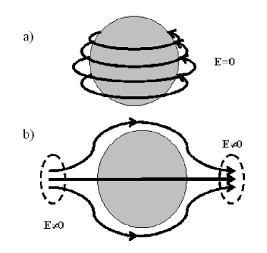
Figure 1: Polarization $\mathbf{s}$ of the liquid around a nearly spherical object. Forceless (a) and longitudinally polarized (b) liquid configurations.

In the linear response approximation the polarization of the liquid is

$$s_{\alpha}(\mathbf{r})=-\sum_{\mathbf{k}\beta}G_{\alpha\beta}^{(s,s)}(\mathbf{k})j_{\beta}(\mathbf{k})\exp(i\mathbf{kr}),$$ (17)

where

$$G_{\alpha\beta}^{(s,s)}=\frac{P_{0}^{-1}}{Ck^{2}+A}\left(\delta_{\alpha\beta}-\frac{4\pi k_{\alpha}k_{\beta}}{k^{2}}\frac{(k^{2}C^{\prime}/4\pi+1)}{(C+C^{\prime})k^{2}+A+4\pi}\right).$$ (18)

The interaction of the two impurities separated by a large distance $\mathbf{R}=\mathbf{r}_{1}-\mathbf{r}_{2}$ is given by

$$\Omega_{L}(R)=-\sum_{k,\alpha,\beta}G_{\alpha\beta}^{(s,s)}(k)j_{\alpha}j_{\beta}=$$

$$=\frac{1}{P_{0}^{2}}\frac{(\mathbf{j}_{1},\mathbf{j}_{2})-3(\mathbf{j}_{1},\hat{\mathbf{R}})(\mathbf{j}_{2},\hat{\mathbf{R}})}{A^{2}\epsilon R^{3}}.$$

This means that the two neutral impurities (16) interact in unscreened fashion as two dipoles in a media with dielectric constant $\epsilon$. The dipole moment $\mathbf{d}$ arises from spontaneous polarization of water around the object: $\mathbf{d}=\mathbf{j}/(AP_{0})$. We call such liquid configurations as longitudinally polarized states, see e.g. Fig.1b for an example of water polarization force lines around a nearly spherical body. For such polarization type the non-vanishing polarization charge exists in a liquid: $\rho_{P}=-P_{0}{\rm div}\mathbf{s}\neq 0$. The induced dipole moment around a microscopic object of the size $R_{0}\lesssim R_{D}$ can be estimated as follows: at small distances $r\lesssim R_{D}$ ($k\rightarrow\infty$), the second term in the correlation function (18) can be neglected and $\mathbf{s}\sim\mathbf{j}/(P_{0}^{2}Cr)$. The linear theory breaks on the surface of the object, $r=R_{0}$, where $s\sim 1$. Therefore $j\sim P_{0}^{2}CR_{0}$, $d\sim P_{0}CR_{0}/A$ and the energy of a pair of chargeless objects can be estimated as

$$\Omega_{L}(R)\sim\frac{C^{2}R_{0}^{2}P_{0}^{2}}{AR^{3}}.$$ (19)

This interaction is long-range and is completely due to the dipole-dipole interaction of the water molecules.

Longitudinal polarization of the liquid also contributes to the solvation energy of a single impurity:

$$\Omega_{solv}=-\sum_{k,\alpha,\beta}j_{\alpha}j_{\beta}G_{\alpha\beta}^{(s,s)}(k)=\Omega_{0}+\Omega_{A},$$ (20)

where $\Omega_{0}$ comes from the first term of Eq.(18), formally diverges and can be estimated as $\Omega_{0}\sim j^{2}P_{0}^{2}k_{max}/C$, where $k_{max}\sim R_{0}^{-1}$ is related to the size of the impurity. The contribution from the second term is finite and is in fact the energy (9) of the polarization electric field: $\Omega_{A}\sim P_{0}^{2}C^{3/2}=50\,kJ/mol$. Since $\Omega_{0}\sim CR_{0}P_{0}^{2}$, $\Omega_{A}\gtrsim\Omega_{0}$ for impurities of sufficiently small size $R_{0}\lesssim R_{D}$, the quantity $\Omega_{A}$ is large and can be called as the activation energy of the longitudinally polarized configuration.

Large value of the activation energy is due to appearance of strong electric fields next to polarized bodies. In fact there is a wide class of liquid configurations with appreciably lower energies due to the absence of polarization charge. This can happen in a system of neutral bodies if a special, the “forceless” (FL), state of molecular dipoles is chosen:

$$\nabla\mathbf{s} = 0,\mathbf{\;E}=0.$$ (21)

Two examples of forceless water configurations around a sphere and a cylinder are shown on Figs. 1a, 2a. The polarization vector in such states is similar to magnetic field in magnetostatics, therefore the asymptotic form of the interaction potential with with external point size water polarizing impurities can be specified using the following form of the interaction potential:

$$\Omega_{ext}=\int(\mathbf{J},\nabla\times\mathbf{s})dV.$$ (22)

where $\mathbf{J}=\sum_{a}\delta(\mathbf{r}-\mathbf{r}_{a})\mathbf{J_{a}}$, $\mathbf{r}_{a}$ is the position of an impurity, and $\mathbf{J}_{a}$ is a vector property of an impurity . The vector $\mathbf{J}_{a}$depends on the details of the surface-water interactions and requires full microscopic calculation for its determination. The energy of interacting bodies is then:

$$\Omega_{FL}=\sum_{k,\alpha,\beta...}G_{\alpha\beta}^{(s,s)}(k)\epsilon_{\alpha\mu\nu}\epsilon_{\beta\mu^{\prime}\nu^{\prime}}k_{\mu}J_{\nu}k_{\mu^{\prime}}J_{\nu^{\prime}},$$

where $\epsilon_{\alpha\beta\gamma}$ is the totally antisymmetric tensor. Using Eq.(18) we find that the contribution of the second term vanishes. At intermediate distances $R\lesssim L_{T}$

$$\Omega_{FL}(\mathbf{R})=\frac{3(\mathbf{J}_{1},\hat{\mathbf{R}})(\mathbf{J}_{2},\hat{\mathbf{R}})-(\mathbf{J}_{1},\mathbf{J}_{2})}{4\pi P_{0}^{2}CR^{3}}$$ (23)

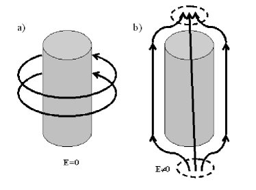
Figure 2: Polarization of a liquid near a cylindrical hydrophobic surface. Forceless (a) and longitudinally polarized (b) liquid configurations.

At larger distances $R\gtrsim L_{T}$ the interaction vanishes exponentially:

$$\Omega_{FL}(\mathbf{R})=\frac{(\mathbf{J}_{1},\hat{\mathbf{R}})(\mathbf{J}_{2},\hat{\mathbf{R}})-(\mathbf{J}_{1},\mathbf{J}_{2})}{4\pi P_{0}^{2}CRL_{T}^{2}}e^{-R/L_{T}}.$$ (24)

The estimation for the vector $\mathbf{J}$ proceeds as follows: at small distances $s\sim J/(P_{0}^{2}CR^{2})$ and has to be $s\sim 1$ at the surface $R\sim R_{0}$ of the body. Hence, $\mathbf{J}_{1,2}=4\pi P_{0}^{2}CR_{1,2}^{2}\mathbf{n}_{1,2}$, where $\mathbf{n}_{1,2}$ are the unit vectors connected with the vorticity of polarization (see Figs. 1a and 2a) by the “right-screw rule”, $R_{1,2}$ are the characteristic radii of the objects. The interaction of a pair of chargeless impurities in a forceless water configuration at small (23) and large (24) distances reads, correspondingly:

$$\Omega_{FL}\sim\frac{CR_{0}^{4}P_{0}^{2}}{R^{3}}$$ (25)

$$\Omega_{FL}\sim\frac{CR_{0}^{4}P_{0}^{2}}{RL_{T}^{2}}e^{-R/L_{T}}.$$ (26)

The exponential decay of the interaction at large distances is not surprising since forceless configurations are also chargeless and the net dipole momentum of the system is identically zero. Note, that for a forceless configuration the polarization of the liquid is present at distances $\lambda\sim L_{T}$ from the solute surface.

Eqs. (25), (26) universally characterize forceless interactions of small neutral objects. In linear approximation (17) the polarization vector around a pair of solutes located at points $\mathbf{\rho}_{1}$ and $\mathbf{\rho}_{2}$ is given by

$$\mathbf{s}(\mathbf{r})\equiv\mathbf{s}_{FL}=R_{1}^{2}(\mathbf{n}_{1}\times\hat{\mathbf{r}}_{1})f(r_{1})+R_{2}^{2}(\mathbf{n}_{2}\times\hat{\mathbf{r}}_{2})f(r_{2}),$$ (27)

where $f(r)=r^{-2}(1+r/L_{T})\exp(-r/L_{T})$. Here $\mathbf{r}_{1,2}=\mathbf{r}-\mathbf{\rho}_{1,2}$, $\hat{\mathbf{r}}_{1,2}=\mathbf{r}_{1,2}/r_{1,2}$, and $R_{1,2}$ are the characteristic radial dimensions of the solute particles. Eq. (27) is valid far from the objects ($r_{1,2}\gg R_{1,2}$). If the solute bodies carry charges, than additional induced polarization contribution appears:

$$\mathbf{s=}\mathbf{s}_{FL}+\mathbf{s}_{P},$$ (28)

$$\mathbf{s}_{P}\sim-\delta_{1}g(r_{1}/R_{D})\hat{\mathbf{r}}_{1}-\delta_{2}g(r_{2}/R_{D})\hat{\mathbf{r}}_{2},$$ (29)

where $g(x)=x^{-2}\left[1-\left(1+x\right)\exp\left(-x\right)\right]$, $\delta_{1,2}=q_{1,2}/q_{C}$. The water polarization is qualitatively represented on the Fig. 3. Water polarization of this type was obtained in MD simulations Higo and called as “the dipole-bridge between biomolecules”. The vortex-like structures of polarization were observed that corresponds to the term $\mathbf{s}_{FL}$ in (28).

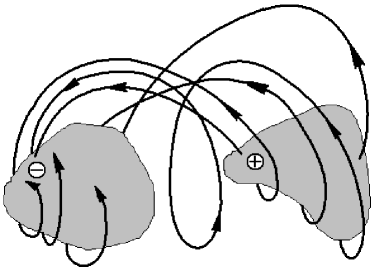
Figure 3: Polarization of a liquid near two hydrophobic charged solutes.

At intermediate distances between the interacting bodies both forceless (FL) and longitudinally polarized (L) liquid configurations have very similar interaction properties. Both $\Omega_{L}$ and $\Omega_{FL}$ are dipole-dipole interactions of polarized molecular dipoles. For sufficiently small impurities we have $\Omega_{FL}/\Omega_{L}\sim R_{0}^{2}/R_{D}^{2}\ll 1$. This means that the interactions of small longitudinally polarized impurities is stronger. On the other hand, the second term of Eq. (18) does not also contribute to the solvation energy of a single forceless impurity, which means that the forceless configurations does not have the large activation energy contribution $\Omega_{A}\gg T$ in its free energy and hence, at least at large distances, thermodynamically is more probable. At intermediate distances, $R\lesssim L_{T}(R_{0}^{2}/R_{D}L_{T})^{1/3}\ll L_{T}$, $\Omega_{L}\gtrsim\Omega_{A}$ and spontaneously polarized liquid configuration with anti-parallel $\mathbf{j}$ possesses lower energy and may become favorable. This means that anisotropic neutral molecules in a polar liquid can acquire fairly strong orientation dependent interaction caused by induced dipole moment of the surrounding water molecules.

III.3 Interaction of macroscopic objects: parallel hydrophobic cylinders.

The interaction potentials (19) and (24) give only the energies of point-like objects of size $R_{0}\ll R_{D}$. In realistic calculations $R_{0}\gtrsim R_{D}$(small organic molecules) and may even be larger (proteins, lipids etc.). For larger objects, a more detailed calculation has to be done. Consider first two parallel cylinders of the same radii $R_{1,2}=R_{0}$, heights $H_{1,2}=H\gg R_{0}$, placed at a distance $L\ll H$ from one another. The separation between the objects is large, $L\gg R_{0}$, but the size $R_{0}$ is now arbitrarily related to the water domain size $R_{D}$. At distances large enough from the cylinder cores the superposition principle holds:

$$\mathbf{s}(\mathbf{r})\approx\mathbf{s}_{1}(\mathbf{r})+\mathbf{s}_{2}(\mathbf{r}),$$ (30)

where $\mathbf{s}_{i}$, are cylindrically symmetric forceless solutions of model around isolated cylinders (see Fig.2a):

$$\mathbf{s}_{i}(\mathbf{r})=\lambda_{i}\frac{R_{i}}{r_{i}}\beta_{i}\hat{\phi_{i}}.$$ (31)

Here $\lambda_{1,2}=\pm 1$ stands for two possible directions of water dipoles around a cylinder (the “topological charges”), $r_{i}$ are the distances from the point $\mathbf{r}$ to the axis of the correspondent cylinder. The coefficients: $\beta_{1,2}\approx 1/\left[1+\gamma R_{1,2}/R_{D}\right]$, where $\gamma\sim 1$ depends on the behaviour of the function $V(s^{2})$ for $s\sim 1$. Formula (31) holds for $r_{i}\ll L_{T}$. Since $\nabla\mathbf{s}\approx 0$, the polarization electric field vanishes. Substituting directly the solution (30) into the energy density (2) we find the following expression for the interaction potential:

$$\Omega_{FL}(L)\approx 2\pi AP_{0}^{2}\lambda_{1}\lambda_{2}\beta_{1}\beta_{2}R_{0}^{2}HK_{0}\left(\frac{L}{L_{T}}\right),$$ (32)

where $K_{0}$ is the Macdonald function. For small cylinders, $R\ll R_{D}$, $\beta\approx 1$ and the result (32) coincides with that one can find by integrating the potential (24) over the cylinders in the linear model. At sufficiently small distance between the cylinders the interaction exceeds the activation energy $\Omega_{A}$ and the longitudinally polarized configuration settles (see Fig. 2b). Here $\nabla\mathbf{s}\neq 0$ close to the ends of the cylinders, so that the energy of each of the cylinders contains $\Omega_{A}\sim 2\pi R_{0}^{2}\sqrt{C}\pi P_{0}^{2}$. The superposition principle still holds and the energy of the cylinders reads:

$$\Omega_{L}(L)\approx 2\pi CP_{0}^{2}\frac{\lambda_{1}\lambda_{2}}{\Lambda_{1}\Lambda_{2}}\beta_{1}\beta_{2}HK_{0}\left(\frac{L}{L_{T}}\right).$$ (33)

Here $\Lambda_{1,2}=\log(L_{T}/R_{1,2})$. The result is again similar to that one can find by integrating the interaction potential for a spontaneously polarized configuration (19) over entire cylinders length.

Eqs.(30) and (31) describe an approximate forceless solution. Let us estimate the leading correction $\Omega^{\prime}$ to the interaction energy due to the dipole-dipole interactions of polarization charges (${\rm div\mathbf{s}}\neq 0$). Consider first two cylinders at a distance $L\ll L_{T}$. In this case the polarization charges are concentrated around the cylinders surface, $Q_{A,B}=-Q_{C,D}\sim P_{0}R_{0}$ in the sectors $A-D$ of Figure 4. The dipole moment $D\sim P_{0}R_{0}L$ per unit length along the cylinders gives the following estimation for the interaction energy

$$\Omega^{\prime}\sim\frac{1}{\epsilon(k\sim L^{-1})}\int dz_{1}dz_{2}\frac{\left[(\mathbf{D}_{1}\mathbf{D}_{2})-3(\mathbf{n}\mathbf{D}_{1})(\mathbf{n}\mathbf{D}_{2})\right]}{r_{12}^{3}}=$$

$$=\frac{2H}{\epsilon(k\sim L^{-1})L^{2}}\left[(\mathbf{D}_{1}\mathbf{D}_{2})-2D_{1x}D_{2x}\right]$$ (34)

The integration in (34) is performed along the axes $z_{1,2}$ of the cylinders. The vector $\mathbf{r}_{12}$ connects the points at the axes, $r_{12}=\sqrt{(z_{1}-z_{2})^{2}+L^{2}}$, and $\mathbf{n=r}_{12}/r_{12}$. For a pair of cylinders of the same size $\mathbf{D}_{1}=\mathbf{D}_{2}\equiv\mathbf{D}$ and

$$\Omega^{\prime}\sim\frac{P_{0}^{2}HR_{0}^{2}(L^{2}+L_{T}^{2})}{\epsilon(L^{2}+R_{D}^{2})}.$$ (35)

At larger distances, $L\gtrsim L_{T}$, the solution (31) acquires an extra exponential factor $\exp(-r/L_{T})$ and

$$\Omega^{\prime}\sim\frac{P_{0}^{2}HR_{0}^{2}}{\epsilon}\exp(-2L/L_{T}).$$

Comparing this result with Eqs.(32) and (35) we find:

$$\Omega^{\prime}(L)/\Omega_{FL}(L)\sim\exp(-L/L_{T})\leq 1.$$

This means that for sufficiently large distances the polarization charges provide negligible corrections to the energy of a forceless configuration.

IV Solvent-solute interfaces. Phase transitions on boundaries.

Consider now the structure of molecular polarization near a plane liquid-to-vacuum or liquid-to-a body surface interface. Such a boundary is hydrophobic and polarizes the liquid along the boundary plane $\Gamma$. The polarization extends to the bulk of the liquid on a distance scale $\lambda\sim L_{T}$ or $\lambda\sim R_{D}$ depending on electrostatic properties of the boundary (see below). Since at larger distances from the boundary the polarization of the liquid disappears, the polarization itself is an effectively two-dimensional vector field. The Hamiltonian for the surface polarization field $\mathbf{s}_{\|}$ can be obtained by integration of (2) inside the bulk of the liquid:

$$\Omega_{S}\approx\frac{1}{2}M\int_{\Gamma}df\left(\nabla\theta\right)^{2}+\frac{1}{2}K\int_{\Gamma}df\left(\nabla\cdot\mathbf{S}\right)\phi(\mathbf{r})$$ (36)

$$\phi(\mathbf{r})=\int_{\Gamma}df^{\prime}\frac{(\nabla^{\prime}\cdot\mathbf{S}^{\prime})}{\left|\mathbf{r}-\mathbf{r}^{\prime}\right|}.$$ (37)

Here $\theta(x,y)$ is the angle characterizing the direction of the unit vector $\mathbf{S}=\mathbf{s}_{\|}/s_{\|}=(\cos\theta,\sin\theta)$, $\mathbf{r}=(x,y)$ are the coordinates along the surface, $\nabla=(\partial/\partial x,\partial/\partial y)$, $\phi(\mathbf{r})$ is the electric potential at the point $\mathbf{r}$. The constants $M\sim CP_{0}^{2}\lambda s_{\|}^{2}$, $K\sim\lambda M$ . Both terms in Eq. (36) originate from $\Omega_{H}$ and $\Omega_{dd}$ of Eq.(2), respectively. Note that

$$\nabla\cdot\mathbf{S}=-\sin\theta\cdot\theta_{x}+\cos\theta\cdot\theta_{y},$$ (38)

where $\theta_{x}\equiv\partial\theta/\partial x$, $\theta_{y}\equiv\partial\theta/\partial y$. Minimization of the functional (36) with respect to the variations of $\theta(x,y)$ gives the following ”equilibrium condition”:

$$M\Delta\theta(x,y)+K(-\sin\theta\cdot\phi_{x}+\cos\theta\cdot\phi_{y})=0$$ (39)

The simplest solutions of the selfconsistent equations (39), (37), (38) is the uniform polarization: $\theta(x,y)={\rm const}$ and

$$\mathbf{S}={\rm const}$$ (40)

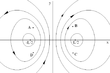
Figure 4: Polarization configuration $\mathbf{S}(x,y)$ of surface water “vortex-antivortex pair”.

A more sophisticated solution describes a vortex state: $\theta(x,y)=m\arctan(y/x)$ of topological charge $q=m=0,\pm 1,\pm 2,...$. Both mentioned solutions are forceless configurations and therefore $\lambda\sim L_{T}$. The vortex core size is also $\sim L_{T}$. Fig.4 shows a more complicated polarization configuration, which is is a vortex-antivortex pair. In this case $\nabla\cdot\mathbf{s}\neq 0$ and thus $\lambda\sim R_{D}$ for all essential configurations with vortex-antivortex pairs.

Let us neglect first the dipole-dipole interaction term $\Omega_{dd}$ in (36). In this case Eq.(36) coincides with the Hamiltonian of XY 2D model. As it is well known from the field theory Berezinskii ; KosterlitzThouless , thermal fluctuations of the polarization field (36) can be mapped on to the thermal dynamics of a gas of interacting vortices residing on the surface. The thermal state of the liquid mainly consists of vortex-antivortex pairs of minimum charge $|q|=1$. The energy of vortex-antivortex configuration at large distance

$$L\gg\lambda$$ (41)

between their cores is given by

$$\Omega(L)\approx\Omega_{1}+\pi M\log\left(L/\lambda\right),$$ (42)

where $\Omega_{1}\sim M$. We observe that the “hydrogen-bonding” term $\Omega_{H}$ leads to appearance of the logarithmic attraction of vortex and antivortex. At temperature

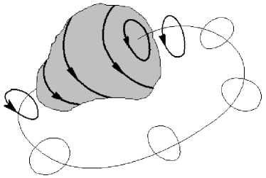
Figure 5: Excitation of water with one vortex-antivortex pair pinned on a surface of hydrophobic solute.

$$T_{BKT}=\frac{1}{2}\pi M\sim\pi CP_{0}^{2}\lambda,$$ (43)

the topological Berezinskii-Kosterlitz-Thouless transition Berezinskii ; KosterlitzThouless occurs: bound vortex-antivortex pairs dissociate and form the vortex “plasma”. According to Onsager arguments Onzager ; Kirkwood ; Frenkel $\epsilon\sim P_{0}^{2}R_{D}^{3}/T$. On a hydrophobic surface $s_{\|}^{2}\sim 1$, and

$$T_{BKT}\sim\epsilon T\gg T.$$ (44)

This means that at any reasonable temperature the polarization field remains ordered (the molecular dipoles are correlated at large distances, see below).

The long-range dipole-dipole interaction described by the second term in Eq.(36) essentially alters the character of BKT transition MaierSchwabl . As is clear from Fig.4 the polarization vector $\mathbf{s}_{1}$ produced by the left vortex encounters other vortex at the region next to the point $C$ and thus induces the polarization density $\rho_{P}(C)>0$. At large distances (41) only one scale $L$ is essential: $\left|\mathbf{r}_{C}-\mathbf{r}_{D}\right|\sim\left|\mathbf{r}_{C}-\mathbf{r}_{B}\right|\sim L$, therefore $\rho_{P}(C)\sim s_{\|}P_{0}/L$. The polarization charges in each of the sectors equal: $Q_{C}=Q_{D}=-Q_{A}=-Q_{B}\sim\rho_{P}(C)\lambda L^{2}\sim s_{\|}P_{0}\lambda L$. Roughly speaking the polarization charge pattern can be approximated by the charge distributions of two equal downward oriented dipole moments $D\sim Q_{C}L\sim s_{\|}P_{0}\lambda L^{2}$ placed at a distance $\sim L$ one from another. Simple estimations give $\Omega_{dd}\sim D^{2}/L^{3}\sim KL$ and

$$\Omega(L)\approx\Omega_{1}+\pi M\log\left(L/\lambda\right)+\ \beta KL,$$ (45)

with $\beta\sim 1$, instead of (42). In other words the dipole-dipole interaction of vortex with antivortex gives additional attraction term with a linear dependence on $L$. The following remark is necessary to explain this interaction. Indeed, the charge distribution on the left side of Fig. 4 is a “mirror reflection” of that on the right side. Such charge distributions repel in vacuum. In the case of a polar liquid interface the polarization charges $Q_{C}$ increase as $L$ increases so that $Q_{C}+Q_{B}=0$ at any $L$. It means that in order to move apart a vortex and antivortex pair, one should produce additional work to polarize the water molecules. The Mayer-Schwabl phase transition occurs at

$$T=T_{MS}=4T_{BKT}.$$ (46)

The phase transition is analogous to that for quark-gluon plasma formation QuarkGluonPlasma : unbound vortices are formed at $T>T_{MS}$. To establish this fact one has to go beyond the approximation of pair interaction of vortices (45). According to (45) the typical dimension of vortex-antivortex pair is: $L_{P}\sim T/K$. The surface concentration of pairs is: $n_{P}\sim\lambda^{-2}\exp(-\Omega_{1}/T)$. At $n_{P}L_{P}^{2}\sim 1$ we have a plasma-like quasineutral system, in which topological charges of vortices and antivotices are mutually compensated. Using our estimations for the parameters $K$, $\Omega_{1}$ and $\lambda$ we conclude that at $T>T_{MS}$ the interaction (45) between two vortices is modified and the phase transition occurs. In fact, Eq. (45) between describes the interaction of vortices only at $T\lesssim T_{MS}$ . At higher temperatures above the phase transition point we can use a set of standard Debye arguments as in linear approximation of screening in plasma (see e.g. LandLifshtiz ). and we find the following mean-field effective interaction between vortices of $Q_{T}$ placed at a distance $L$ from each other :

$$\Omega(L)=Q_{T}^{2}\int_{0}^{\infty}dpp\frac{pJ_{0}(pL)}{(p^{2}+\kappa^{2})p+\kappa^{2}p_{1}}.$$

Here $\kappa=\sqrt{2\pi n_{P}M/T}\sim 1/\lambda$ and $p_{1}=K/(\pi M)\sim 1/\lambda$. Note that $\kappa\sim p_{1}$ at $T\sim T_{MS}$. At $T\gg T_{MS}$ $\kappa\gg p_{1}$, and at small distances, $L\ll 1/p_{1}$, the the interaction is logarithmic: $\Omega(L)\approx\pi MK_{0}(\kappa L)+\beta KL$ , which recovers Eq. (45) at sufficiently small distances $L\ll 1/\kappa$. At large distances $L\gg 1/p_{1}$ the screening switches on and the interaction decays as $\Omega(L)\approx Q_{T}/(\kappa^{2}p_{1}L^{3})\sim 1/L^{3}$.

Eqs. (44) and (44) show clearly that the phase transition can not be observed on a hydrophobic surface. Nevertheless it may occur on hydrophilic surfaces, where the energy of the liquid can be further lowered by extra-hydrogen bonds involving the atoms on the surface of the solute. In a place of such polar contact the vector $\mathbf{s}$ is almost perpendicular to the liquid boundary: $s_{\|}^{2}\ll 1$. The effective Hamiltonian for the molecular dipole field on a hydrophilic surface still has the form (36), though the phase transition temperature is lower: $T_{MS}\sim CP_{0}^{2}\lambda s_{\|}^{2},$ $T_{MS}/T\sim\epsilon s_{\|}^{2}$. The appearance of the additional small factor $s_{\|}^{2}$ can decrease $T_{MS}$ drastically: the transition temperature may be shifted to the room temperatures range already on a hydrophilic surface with $s_{\|}\sim 0.1$.

At $T\gtrsim T_{MS}$ the vortices dissociate and form vortex-antivortex plasma, so that the order parameter $\mathbf{s}$ fluctuates strongly. One may say that at small temperatures (or on a highly hydrophobic boundary) the molecular dipoles fluctuations are small and the molecular directions field is highly ordered on large scales. In other words global network of hydrogen bonds exist on the surface of the solute body. As the polar interactions of the solute object and the surrounding liquid increase, the the phase transition temperature gets lower and the global polarization order, and hence the hydrogen bonds network, disintegrates. Moreover the hydrophilic regions on the surface of the solute may pin the vortices, giving rise to a peculiar sophisticated polarization shapes (see Fig. (5) and the discussion in Higo ).

We argue that the above discussed phase transition is directly related to the disruption of the global hydrogen bonds network in the course of 2D percolation phase transition observed in the Molecular Dynamics simulation of hydration water absorbed on the surface of a solute Oleinikova1 ; Oleinikova2 ; Oleinikova3 . In our model this result can be explained with the help of classical field theory considerations. At $T>T_{MS}$ a solute boundary hosts a gas of independent vortices of different “circulation” resulting in fast decay of correlation between dipole moments of distant water molecules: $D(\mathbf{r})=\left\langle\mathbf{d}(0)\mathbf{d}(\mathbf{r})\right\rangle\sim\exp\left(-r/r_{C}\right)$ MaierSchwabl . At $T<T_{MS},$ the vortices annihilate the and long-range correlations set in: the ferromagnetic-like ordering of hydration water molecules dipole moments takes place. It means that in the considered case of polar liquids the boundary layer of liquid is a ferroelectric film. Such correlated thermal states can be seen as global network of hydrogen bonds at the surface. Note that in our model the value of transition temperature $T_{MS}$ is proportional to the width of polarized layer $\lambda$, which is in accordance with the dependence of percolation transition temperatures obtained in Oleinikova1 ; Oleinikova2 ; Oleinikova3 as a function the hydration shell width $D$ (of course, it is reasonable to suppose that $D\sim\lambda$).

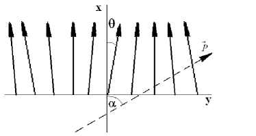
Figure 6: Ferroelectric wave propagates in a film of hydration water.

The appearance of ferroelectric order can be used as a justification for the mean field picture employed throughout the Letter. This fact does not contradict with the Peierls-Mermin theorem Peierls ; Mermin on the absence of ordering in a 2D systems due to new effect: the long-range dipole-dipole term in (36). To illustrate this point consider collective vibrations of molecular dipole moments in a ferroelectric hydration water layer (Fig.6) with molecular dipoles arranged along $x$ axis. The kinetic energy of a water molecule is $I\dot{\theta}^{2}/2$, where $I$ is the molecular moment of inertia. The dispersion law $\omega=\omega(\mathbf{p})$ of the ferroelectric wave of a wave vector $\mathbf{p}$ can be established by the minimization of the action $S=\int Ldt$, where the Lagrangian $L$ reads

$$L=\int df\frac{1}{2}N\dot{\theta}^{2}-\Omega_{S}.$$

Here $N=\lambda nI$ and the interaction potential $\Omega_{S}$ is defined by (36). The equation of motion

$$-N\ddot{\theta}+M\Delta\theta(x,y)+K(-\sin\theta\cdot\phi_{x}+\cos\theta\cdot\phi_{y})=0$$

can be expanded in powers of small $\left|\theta\right|\ll 1$ so that the dispersion relation is:

$$\omega(\mathbf{p})=\sqrt{\frac{Mp^{2}}{N}+\frac{2\pi K}{N}p\sin^{2}\alpha}.$$ (47)

Here $\alpha$ is the angle between vector $\mathbf{p}$ and $x$ axis. Consider the Peierls-Mermin argument applied for a 2D atomic crystalline lattice. Mean squared displacements of the atoms from the equilibrium positions in the lattice are proportional to the integral $J=\int d^{2}p/\omega^{2}(\mathbf{p})$. Short-range interactions of atoms give the phonon excitations with $\omega\sim p$. In this case $J$ diverges at small values of $p$, which corresponds to fluctuations with large wave lengths. The integral with the dispersion relation (47) does not have the singularity at small $p$:

$$J\sim\int_{0}^{2\pi}d\alpha\int_{0}^{\infty}dp/(Mp+2\pi K\sin^{2}\alpha)\sim\int_{0}^{\infty}dp/\sqrt{p},$$ (48)

which means that the long-range dipole-dipole together with the short-range hydrogen bonding interaction both stabilize the ferroelectric ordering of the film in agreement with MaierSchwabl . Interestingly both $\Omega_{H}$ and $\Omega_{dd}$ are equally important in this phenomenon: long range order does not exist both in the film with the short and the long range interactions separately: the integral diverges either if $M=0$ (no short range hydrogen bonds in the model) and if $K=0$ (no dipole-dipole interaction). This somewhat surprising observation means that the short-range behavior of intermolecular interactions determine the character of order at large scales. Physically it is a consequence of the Earnshaw’s instability of the system of classical dipoles, which is stabilized by the H-bonds. Similar findings are reported in Belobrov ; Brankov ; Zimmerman ; Bedanov where the 2D system of classical dipoles were considered on a few different types of lattices. It was shown that the ground state of the lattice system can switch from a ferromagnetic to antiferromagnetic state depending on the lattice shape.

V Concluding remarks.

Finally we compare the results of our vector model to the density functional theory, which is another well known approach to hydrophobic interactions calculations. It was pioneered in earlier works of van Der Waals vdW , works well for simple, non polar liquids with $\epsilon\sim 1$, does not focus on electric properties and uses the free energy functional expressed in terms of the mean $n(\mathbf{r})=\langle\rho(\mathbf{r})\rangle$, the total $\rho(\mathbf{r})$ density of the liquid, and the density fluctuations $\omega(\mathbf{r})$ ($\langle\omega(\mathbf{r})\rangle=0$) Chandler ; Lum ; Wolde ; Rowlinson ; Nechaev . The free energy functional for the mean density is a non-linear function of $n(\mathbf{r})$ and is characterized by the healing length $a_{mac}\sim 7\textrm{\r{A}}$ for water. The fluctuations $\omega(\mathbf{r})$ are described by the pair correlation function taken from experiments or molecular dynamics simulations and is characterized by the second, microscopic scale, $a_{mic}\sim 1\textrm{\r{A}}$. If the interaction between the molecules of a liquid is purely short range, the correlation function for the fluctuations decays exponentially at large distances:

$$G=\langle\omega(0)\omega(\mathbf{r})\rangle\sim\frac{\exp(-r/a_{mic})}{r}.$$

The interaction potential $\Omega$ of a pair of point-like objects is proportional to the correlation function, $\Omega(r)\sim G(r)\sim\exp(-r/a_{mic})$ and, due to the scalar nature of underlying theory, is not orientation dependent. Technically speaking the model suggested in this paper also describes a model system with two characteristic scales, say, $a_{mac}\sim L_{T}$ and $a_{mic}\sim R_{D}$ and thus can share many predictions with the density functional models. On the other hand, as was shown above the long-range dipole-dipole interaction between the molecules of the liquid leads to a long-range power-law tail in the correlation function (18):

$$\langle s_{\alpha}s_{\beta}\rangle\sim\frac{1}{r^{3}},\,r\rightarrow\infty.$$

This property is inherently related with the large dielectric constant and is directly responsible for the strong long-range orientation-dependent interactions described in this Article. Strictly speaking the liquid in our model is incompressible, the assumption obviously fails at $r\sim a_{mic}$. The complete model should include both fluctuations of the liquid density (scalar) and the polarization (vector). One example of such a model of a polar liquid was studied in Ramirez . Molecules were considered as freely oriented, like in the Onzager’s theory Onzager ; Kirkwood ; Frenkel . The approach proved to successfully reproduce the results of molecular dynamics simulations for solvated ions. Another route to include the effects of liquid polarization and electrostatic forces in the scalar model is outlined in Nechaev . The advantage of vector models is clearly seen when the effects of the molecular polarization need to be taken into account, e.g. in a case of charged solutes or for liquid boundaries and interfaces. No scalar model can be directly applied to hydrogen bonds network formation studies and topological excitations and interactions both in the bulk and on the solute boundaries.

The proposed vector model is both physically rich, relatively simple, and is not much more computationally demanding than continuous solvation models used in computational biophysics (see, e.g. Karplus ; Onufriev ). In its linearized form it reproduces a few very important features of molecular dynamics simulations, such as spontaneous liquid polarization next to macroscopic surfaces, the vortex-like structures in the molecular dipoles arrangement near soluted bodies. Strong interaction between the liquid molecules selects forceless liquids configurations with vanishing polarization electric field. This leads to a strong, long-range, orientation dependent interaction of solvated bodies. The model may serve well as a continuous water model to describe different operational states of nanodevices in aqueous environments, as well as membrane charge transfer and ion channels, where both the hydrophobic and charged boundaries are equally important.

Fast solvation models are crucial in drug discovery and biomolecules modelling. The quality of solvation models is a limiting factor determining the accuracy of the calculations in molecular docking and virtual screening applications. The proposed model is employed in QUANTUM drug discovery software for very accurate binding affinity predictions for protein-ligand complexes qpharm . QUANTUM uses the continuous vector water model (2) for solvation energy predictions, determination of protonation states of biomacromolecules, pKa calculations, protein structure refinement (including mutagenesis) etc.

References

- (1) D.C. Rapaport, Computer Physics Communications, , 198 (1991); , 217 (1991); , 301 (1993)
- (2) Schaefer M., Karplus M., J.Chem.Phys. , 1578(1996)
- (3) M. Feig, A. Onufriev, M.S. Lee, W. Im, D. A. Case, C. L. Brooks, J. Comp. Chem., 498, 96 (2004)
- (4) Chandler D., Phys.Rev. E 48, 2898(1993)
- (5) Lum K., Chandler D., Weeks J.D., J.Chem.Phys. B 103, 4570 (1999)
- (6) Wolde P.R., Sun S.X., Chandler D., Phys.Rev. E 65, 011201 (2001)
- (7) Lee C.Y., McCammon J.A., Rossky P.J., J. Chem. Phys. 80, 4448 (1984)
- (8) Wilson M.A., Pohorille A., Pratt L.R., J. Chem. Phys. 91, 4873 (1987)
- (9) Kohlmeyer A., Hartnig C., Spohr E., J. Mol. Liquids. 78, 233 (1998)
- (10) J. Higo, M. Sasai, H. Shirai, H. Nakamura, T. Kugimiya, www.pnas.org/cgi/doi/10.1073/pnas.101516298
- (11) A. Oleinikova, N. Smolin, I. Brovchenko, A. Geiger, R. Winter, J. Phys. Chem. B , 1988 (2005)
- (12) A. Oleinikova, I. Brovchenko, N. Smolin, A. Krukau, A. Geiger, R. Winter, cond-mat/0505564, 2005
- (13) A. Oleinikova, I. Brovchenko, A. Geiger, cond-mat/0507718, 2005
- (14) Ginzburg V.L., Zh.Eksp.Teor.Fiz. 15, 739 (1945); J.Phys.USSR 10, 107(1946)
- (15) Sivukhin D.V., General Course of Physics. V. 3, Electricity. Moscow, Nauka-Fizmatlit, 1996
- (16) Stratton J.A., Electromagnetic Theory. McGraw-Hill, New York, 1941
- (17) Kolafa J., Nezbeda I., Mol.Phys.97, 1105(1999); 98, 1505(2000)
- (18) Gray C.G., Gubbins K.E., Theory of Molecular Fluids. Clarendon Press, Oxford, 1984
- (19) L.D.Landau, E.M.Lifshitz, Statistical Physics. Part 1 (Vol. 5), (Pergamon Press, 1969)
- (20) Pauling L., General Chemistry. Dover Publications, 3nd ed. 2003
- (21) A. Stogrin, IEEE Transactions of Microwave Theory Tech., Vol. MTT-19, 733 (1971)
- (22) D.A. Boyarskii, V.V. Tikhonov., N.Yu. Komarova, Progress in Electromagnetic Research, PIER, , 251 (2002)
- (23) G.N. Zatsepina, Physical Properties and Structure of Water. Moscow State University, Moscow, 1998
- (24) L.D. Landau, E. M. Lifshitz, and L.P. Pitaevskii, Electrodinamics of continuum media (Pergamon Press, 1969)
- (25) Ramirez R., Gebauer R., Mareschal M., Borgis D., Phys.Rev. E 66, 031206 (2002)
- (26) If a solute charge exceeds the linear model breaks down close to the charged molecules and the adjacent water molecules may become “frozen”. The discussion of this phenomena will be published elsewhere.
- (27) V.L. Berezinskii, Sov. Phys. JETP, 493 (1971); 610 (1972)
- (28) J.M. Kosterlitz, D.J. Thouless, J. Phys. C , 1181 (1973)
- (29) Onzager R., J.Amer.Chem.Soc. 58, 1486(1936)
- (30) Kirkwood J.G., J.Chem.Phys. 2, 351(1934); 7, 919(1939)
- (31) Frenkel Ya.I., Kinetic Theory of Liquids. Moscow-Ijevsk, NIC Regular and Chaotic Dynamics, 2004
- (32) P.G. Maier, F. Schwabl, Phys.Rev. B , 134430 (2004)
- (33) Kittel W., De Wolf E.A. Soft Multihadron Dynamics (Singapore: World Scientific, 2005)
- (34) Peierls R.E. Ann. Inst. Henry Poincare, , 122 (1935)
- (35) Mermin N.D. Phys. Rev. , 250 (1968)
- (36) Belobrov P.I., Voevodin V.A., Ignatchenko V.A. Zh.Exper.Teor.Fiz. , 3673 (1985)
- (37) Brankov J.G., Danchev D.M. Physica A , 128 (1987)
- (38) Zimmerman G.O., Ibrahim A.K., Wu F.Y. Phys. Rev. B , 2059 (1988)
- (39) Bedanov V.M. J.Phys.: Condens. Matter, , 75 (1992)
- (40) van der Waals J.D., Ph.Constamm, Lehrbuch der Thermostatik. Verlag von Johann Ambrosius Barth, Leipzig, 1927
- (41) Rowlinson J.S., Widom B., Molecular theory of capillarity. Clarendon Press, Oxford, 1982
- (42) Sitnikov G., Nechaev S., Taran M., Muryshev A., Application of a two-length scale field theory on the solvation of charged molecules: I. Hydrophobic effect revisited. arXiv: cond-mat/0505337 v2 14 May 2005
- (43) http://q-pharm.com, see http://q-pharm.com/home/contents/sci_and_tech/proof of concept page for the binding affinity calculations accuracy assessment.