Non-Gaussian energy landscape of a simple model for strong network-forming liquids: Accurate evaluation of the configurational entropy.

Abstract

We present a numerical study of the statistical properties of the potential energy landscape of a simple model for strong network-forming liquids. The model is a system of spherical particles interacting through a square well potential, with an additional constraint that limits the maximum number of bonds, $N_{\rm max}$, per particle. Extensive simulations have been carried out as a function of temperature, packing fraction, and $N_{\rm max}$. The dynamics of this model are characterized by Arrhenius temperature dependence of the transport coefficients and by nearly exponential relaxation of dynamic correlators, i.e. features defining strong glass-forming liquids. This model has two important features: (i) landscape basins can be associated with bonding patterns; (ii) the configurational volume of the basin can be evaluated in a formally exact way, and numerically with arbitrary precision. These features allow us to evaluate the number of different topologies the bonding pattern can adopt. We find that the number of fully bonded configurations, i.e. configurations in which all particles are bonded to $N_{\rm max}$ neighbors, is extensive, suggesting that the configurational entropy of the low temperature fluid is finite. We also evaluate the energy dependence of the configurational entropy close to the fully bonded state, and show that it follows a logarithmic functional form, differently from the quadratic dependence characterizing fragile liquids. We suggest that the presence of a discrete energy scale, provided by the particle bonds, and the intrinsic degeneracy of fully bonded disordered networks differentiates strong from fragile behavior.

I. INTRODUCTION

When a liquid is fastly supercooled into a metastable state under the melting point, its structural relaxation time, $\tau$, increases over 13 orders of magnitude with decreasing temperature, $T$. Below some given temperature, equilibration is not possible within laboratory time scales and the system becomes a glass debenedettibook ; binder . The glass transition temperature, $T_{\rm g}$, is operationally defined as that where $\tau=100$ seconds, or the viscosity $\eta=10^{13}$ poise.

Angell has introduced a useful classification scheme fragdef for glass-forming liquids. According to the definition of kinetic fragility, a liquid is classified as ‘strong’ or ‘fragile’ depending on how fast its relaxation time increases when approaching $T_{\rm g}$. Liquids that show a weak dependence, well described by an Arrhenius law $\tau\propto\exp(A/T)$, with $A$ a temperature independent quantity, are classified as strong. Strong liquids form open network structures that do not undergo strong structural changes with decreasing temperature. On the contrary, the dynamics of fragile liquids, as many polymeric or low molecular weight organic liquids, where interactions show a less directional character, are more sensitive to temperature changes, and relaxation times show strong deviations from Arrhenius behavior bohmer ; martinez . Several empirical functions have been proposed for the $T$ dependence of $\tau$ in fragile liquids, the Vogel-Tammann-Fulcher (VTF) law, $\tau\propto\exp[A/(T-T_{0})]$, having gained more acceptance vtf . In this equation $T_{0}$ is the VTF temperature.

Kauzmann noted kauzmann that, when extrapolating to low temperature the experimental $T$ dependence of the configurational entropy, $S_{\rm conf}$, the latter became zero at a certain temperature $T_{\rm K}$ (‘Kauzmann temperature’) somewhere below $T_{\rm g}$. Experiments debenedettibook ; notetk often provide the result $T_{\rm K}\approx T_{0}$. Given the Arrhenius character of strong liquids, this comparison would also suggest that $T_{\rm K}$ is zero for these systems.

However, it must be stressed that the values of $T_{\rm K}$ and $T_{0}$ are the result of an extrapolation of experimental data, which in principle is not necessarily correct. In particular, an extrapolation below $T_{\rm K}$ would lead to an ‘entropy catastrophe’: a disordered liquid state with less entropy than the ordered crystal. In practice, the equilibrium liquid state at the putative $T_{\rm K}$ is never reached in experiments, because the liquid falls out of equilibrium at $T_{\rm g}>T_{\rm K}$. The fate of the configurational entropy in an ideal situation where arbitrarely long equilibration time scales could be accessed is one of the key (and controversial) questions associated to the glass transition problem. One solution states that crystallization is unavoidable when approaching $T_{\rm K}$ in equilibrium kauzmann ; cavagna . It has also been proposed that $S_{\rm conf}$ changes its functional form below $T_{\rm g}$, remaining always positive stillingertk . Another solution is that $S_{\rm conf}$ reaches zero at $T_{\rm K}$ and remains constant below it gibbsdimarzio ; derrida ; wolynes ; mezard .

Some insight into this latter question, in the physical origin of the fragility, and in general in the relation between dynamic and thermodynamic properties of glass-forming liquids, can be obtained by investigating the potential energy landscape (PEL) goldstein ; stillinger-pel ; stillinger-rev ; wales ; angell95 ; jstat , i.e., the topology of the potential energy of the liquid $U=U({\bf r}^{N})$. According to the inherent structure (IS) formalism introduced by Stillinger and Weber stillinger-pel , the PEL is partitioned into basins of attraction around the local minima of $U$. These minima are commonly known as the ‘inherent structures’. The free energy is obtained as a sum of a ‘configurational’ contribution, resulting from the distribution and multiplicity of the different IS’s, and another ‘vibrational’ contribution, resulting from the configurational volume available within the basin around each individual IS. The introduction of the IS formulation has motivated a great theoretical and computational effort in order to understand the connection between the statistical properties of the PEL and the dynamic behavior of supercooled liquids sastrynat98 ; st ; buchner1 ; angelani00 ; grigera ; scala ; fdt01 ; sastry01 ; debenedetti01 ; voivod01 ; middleton ; lanave01 ; starr01 ; press ; mossaotp ; keyes ; fabricius ; angelani03 ; doliwa ; vogel ; denny ; newheuer ; ruocco ; angelanientro ; attili , and nowadays has become a key methodology in the field of the glass transition.

From a series of numerical investigations in models of fragile liquids, it is well established that for such systems the distribution of inherent structures is well described by a Gaussian function, at least in the energy range that can be probed within the equilibration times permitted by computational resources st ; sastry01 ; attili . It can be formally proved derrida ; heuer00 that for a Gaussian landscape the energy of the average visited IS depends linearly on $T^{-1}$, a result that has been verified in several numerical studies of fragile liquids sastry01 ; starr01 ; press ; buchner1 ; mossaotp . Recent studies of the atomistic BKS model for silica voivod01 ; newheuer , the archetype of strong liquid behavior, have shown instead that deviations from Gaussianity take place in the low energy range of the landscape, and indeed, at low temperature, the average inherent structure progressively deviates from linearity in $T^{-1}$. The existence of a lower energy cut-off and a discrete energy scale, as it would be expected for a connected network of bonds, has been proposed as the origin of such deviations from Gaussianity newheuer . These investigations also suggest that $S_{\rm conf}$ cannot be extrapolated to zero at a finite $T$, and as a consequence, strong liquids would not show a finite $T_{\rm K}$. However, long equilibration times prevent the determination of the lowest-energy state and its degeneracy, and therefore an unambiguous confirmation of this result.

Recently, we have proposed a minimal model which we believe capture the essence of the prototype strong liquid behavior. In this model moreno , particles interact via a spherical square-well potential with an additional constraint on the maximum number of bonded neighbors, $N_{\rm max}$, per particle. The lowest-energy state is the fully bonded network and its energy is thus unambiguously known. Within the equilibration times permitted by present day numerical resources, configurations with more than 98 per cent of the bonds formed can be properly thermalized. As a result, no extrapolations are required to determine the low $T$ behavior. This model is particularly indicated for studying the statistical properties of the landscape. In analogy with the Stillinger-Weber formalism, we propose to partition the configuration space in basins which, for the present case, can be associated with bonding patterns. A precise definition of the volume in configuration space associated to each bonding pattern can be provided, since a basin is characterized by a flat surface with energy proportional to the number of bonds. Crossing between different basins can be associated to bond-breaking or bond-forming events. In contrast to other systems previously investigated, the vibrational contribution of the PEL can be expressed in a formally exact way. No approximation for the shape of the basins is requested. As we discuss in the following, the precision of the evaluation of the basin volume, only limited by the numerical accuracy of statistical averages, allows us to evaluate, with the same precision, the configurational entropy.

In this article we report the study of the statistical properties of the $N_{\rm max}$ model for the cases $N_{\rm max}=3$, 4 and 5, and for a large range of packing fractions $\phi$, extending the results limited to a fixed $\phi$ and $N_{\rm max}=4$ previously reported in a short communication moreno . The range of $\phi$ values here investigated are (0.2-0.35) for $N_{\rm max}=3$, (0.3-0.5) for $N_{\rm max}=4$, and $\phi=0.35$ for $N_{\rm max}=5$. The article is organized as follows. In Section II we introduce the model and provide computational details. In Section III we briefly summarize the IS formalism and apply it to the present model. Dynamic and energy landscape features are shown and discussed in Section IV. Conclusions are given in Section V.

II. MODEL AND EVENT-DRIVEN MOLECULAR DYNAMICS

The model we investigate is similar in spirit to one previously introduced by Speedy and Debenedetti speedymaxval . In the present model, particles interact through a spherical square-well potential with a constraint on the maximum number of bonds each particle can form with neighboring ones. Namely, the interaction between any two particles $i$ and $j$ that each have less than $N_{\rm max}$ bonds to other particles, is given by a spherical square-well potential of width $\Delta$ and depth $-u_{0}$:

$$V_{ij}(r)=\begin{cases}~{}~{}\infty~{}~{}~{}~{}~{}~{}~{}\hskip 2.27621ptr<\sigma\\ -u_{0}~{}~{}~{}~{}~{}~{}~{}\sigma<r<\sigma+\Delta\\ ~{}~{}~{}0~{}~{}~{}~{}~{}~{}~{}~{}r>\sigma+\Delta,\end{cases}$$ (1)

with $r$ the distance between $i$ and $j$. When $\sigma<r<\sigma+\Delta$, particles $i$ and $j$ form a bond, unless at least one of them is already bonded to other $N_{\rm max}$ particles. If this is the case $V_{ij}(r)$ is simply a hard sphere (HS) interaction:

$$V_{ij}(r)=\begin{cases}~{}~{}\infty~{}~{}~{}~{}~{}~{}~{}~{}r<\sigma\\ ~{}~{}~{}0~{}~{}~{}~{}~{}~{}~{}~{}\hskip 2.27621ptr>\sigma.\end{cases}$$ (2)

In the original model introduced by Speedy and Debenedetti speedymaxval an angular constraint was imposed by avoiding three particles bonding loops. In an effort to grasp the basic structural ingredients originating strong liquid behavior, we have not implemented this additional constraint. The potential given by Eqs. (1, 2), despite its apparent simplicity, is not pairwise additive, since at any instant, the interaction between two given particles does not only depends on $r$, but also on the number of particles bonded to them (if $\sigma<r<\sigma+\Delta$). Hence, to propagate the system it is requested not only the coordinates and velocities, but also the list of bonded interactions.

We also note that the model is not deterministic. Consider a configuration in which particle $i$ is surrounded by more than $N_{\rm max}$ other particles within a distance $\sigma<r<\sigma+\Delta$. Of course, only $N_{\rm max}$ of these neighbors are bonded to $i$, i.e. feel the square-well interaction. If one of the bonded neighbors moves out of the square-well interaction range (i.e. to a distance $r>\sigma+\Delta$), a bond-breaking process occurs. According to Eq. (1), a new bond can be formed with one of the other non-bonded particles whose position is in the range $\sigma<r<\sigma+\Delta$. If several candidates are available —where a candidate is defined as a particle whose distance from $i$ is in the range $\sigma<r<\sigma+\Delta$ and which is engaged in less than $N_{\rm max}$ bonds to other distinct particles — then one of them is randomly selected to form the new bond with the particle $i$. Of course, in each bond-breaking/formation process the velocities of the two involved particles are changed to conserve energy and momentum (see also below).

Despite these complications, the model given by Eqs. (1, 2) can be considered among the simplest ones for simulating clustering and network formation in fluids duda ; huerta . It does not require three-body angular forces or non-spherical interactions. The penalty for retaining spherical symmetry is the complete absence of geometrical constraints between the bonds.

The maximum number of bonds per particle is controlled by tunning $N_{\rm max}$. For a system of $N$ particles, the lowest-energy state, corresponding to the fully bonded network, has an energy $E_{\rm fb}=-NN_{\rm max}u_{0}/2$. If $N_{\rm bb}$ is the number of broken bonds for a given configuration of the network, the energy of that configuration is given by $E=E_{\rm fb}+N_{\rm bb}u_{0}$.

The model parameters have been set to $\Delta/(\sigma+\Delta)=0.03$, $u_{0}=1$ and $\sigma=1$. In the following, entropy, $S$, will be measured in units of $k_{\rm B}$. Setting $k_{\rm B}=1$, potential energy, $E$, and temperature, $T$, are measured in units of $u_{0}$. Distances are measured in units of $\sigma$. Diffusion constants and viscosities are respectively measured in units of $\sigma(u_{0}/m)^{1/2}$ and $(mu_{0})^{1/2}\sigma^{-2}$. We have simulated a system of $N=10000$ particles of equal mass $m=1$, implementing periodic boundary conditions in a cubic cell of length $L_{\rm box}$. We have evaluated the PEL properties for several values of $N_{\rm max}$, in a wide range of $T$, and packing fraction $\phi=\pi N/6L_{\rm box}^{3}$. The system does not exhibit phase separation for the state points here investigated gel ; gellong ; gelgenova .

Dynamic properties are calculated by molecular dynamics simulations. We use a standard event-driven algorithm rapaport for particles interacting via discontinuous step potentials. The algorithm calculates, from the particle positions and velocities at a given instant $t_{0}$, the instants $t_{\rm coll}$ and positions for all possible collisions between distinct pairs, and selects the one which occurs at the smallest $t_{\rm coll}$. Then the system is propagated for a time $t_{\rm coll}-t_{0}$ until the collision occurs. Between collisions, particles move along straight lines with constant velocities. Collisions can take place at relative distance $r=\sigma$ (in which case velocities of colliding particles are reversed according to hard-sphere rules) and, only for bonded interactions, at distance $\sigma+\Delta$ (in which case velocities are changed in such a way to conserve energy and momentum). Starting configurations are selected from previously generated hard-sphere configurations with hard-sphere radius $\sigma+\Delta$. In this way, we start always from a configuration where no bonds are present. After thermalization at high $T$ using the potential defined in Eqs. (1, 2), the system is quenched and equilibrated at the requested temperature. Equilibration is achieved when energy and pressure show no drift, and particles have diffused, in average, several diameters. We also confirm that dynamic correlators and mean squared displacements show no aging, i.e., no time shift when being evaluated starting from different time origins. Once the system is equilibrated, a constant energy run is performed for production of configurations, from which diffusivities and dynamic correlators are computed. Statistical averages are performed over typically 50-100 independent samples. Standard Monte Carlo (MC) simulations are carried out for the calculation of the vibrational contribution of the PEL (see Section III), using previously equilibrated configurations.

III. INHERENT STRUCTURE FORMALISM

If $U=U({\bf r}^{N})$ is the potential energy of a system of $N$ identical particles of mass $m$, the partition function is given by the product $Z=Z^{\rm ig}Z^{\rm ex}$, where $Z^{\rm ig}$ is the purely kinetic ideal gas contribution, and $Z^{\rm ex}$ is the excess contribution resulting from the interaction potential. The ideal gas contribution to the free energy, $F^{\rm ig}=-k_{\rm B}T\ln Z^{\rm ig}$, is given by:

$$\beta F^{\rm ig}/N=\ln(N/V)+3\ln\Lambda-1,$$ (3)

where $V$ is the system volume, $\beta=(k_{\rm B}T)^{-1}$, and $\Lambda=h(2\pi mk_{\rm B}T)^{-1/2}$ is the de Broglie wavelength, with $h$ the Planck constant. The excess contribution to the partition function is:

$$Z^{\rm ex}=\int d{\bf r}^{N}\exp[-\beta U({\bf r}^{N})].$$ (4)

The IS formalism introduced by Stillinger and Weber stillinger-pel , provides a method for calculating $Z^{\rm ex}$. According to Stillinger and Weber the configuration space is partitioned into basins of attraction of the local minima of the PEL, the so-called inherent structures. If $\Omega(E_{\rm IS})$ is the degeneracy of a given IS, i.e., the number of local minima of $U({\bf r}^{N})$ with potential energy $E_{\rm IS}$, the configurational entropy is defined as $S_{\rm conf}(E_{\rm IS})=k_{\rm B}\ln[\Omega(E_{\rm IS})]$. To properly evaluate $Z^{\rm ex}$, besides the information of the number of distinct IS’s, it is necessary to evaluate the partition function $Z^{\rm ex}_{\rm vib}(T,E_{\rm IS})$ constrained in the volume of each of these basins. The quantity $Z^{\rm ex}_{\rm vib}(T,E_{\rm IS})$ provides a measure of the configurational volume explored at temperature $T$ by the system constrained in the basin of depth $E_{\rm IS}$. Averaging over all basins with the same depth $E_{\rm IS}$ one obtains stillinger-pel :

$$Z^{\rm ex}_{\rm vib}(T,E_{\rm IS})=\hskip 85.35826pt$$

$$\frac{1}{\Omega(E_{\rm IS})}\sum_{{\rm basins}(E_{\rm IS})}\int_{\rm basin}d{\bf r}^{N}e^{-\beta(U-E_{\rm IS})},$$ (5)

where the notation “basins($E_{\rm IS}$)” recalls that the sum is performed over all the basins whose potential energy minimum is $E_{\rm IS}$, and each integral runs over the configurational volume associated to the corresponding basin. It is convenient to express $Z^{\rm ex}_{\rm vib}(T,E_{\rm IS})$ as:

$$Z^{\rm ex}_{\rm vib}(T,E_{\rm IS})=e^{-\beta f^{\rm ex}_{\rm vib}(T,E_{\rm IS})},$$ (6)

to stress that the ‘free energy’, $f^{\rm ex}_{\rm vib}(T,E_{\rm IS})$, commonly referred as the vibrational PEL contribution, accounts for the vibrational properties of the system constrained in a typical basin of depth $E_{\rm IS}$.

Within the above framework, the excess partition function is given by:

$$Z^{\rm ex}=\sum_{\rm IS}e^{-\beta[E_{\rm IS}-TS_{\rm conf}(E_{\rm IS})+f^{\rm ex}_{\rm vib}(T,E_{\rm IS})]}.$$ (7)

In the thermodynamic limit the excess free energy, $F^{\rm ex}=-k_{\rm B}T\ln Z^{\rm ex}$, can be evaluated as:

$$F^{\rm ex}(T)=E(T)-TS_{\rm conf}(E(T))+f^{\rm ex}_{\rm vib}(T,E(T)),$$ (8)

where $E(T)$ is the average IS potential energy at temperature $T$. Therefore, the excess free energy is the sum of three contributions. The fist term in Eq. (8) accounts for the average value of the visited local minima of the potential energy. The second term is related to the degeneracy of the typical minimum. The third term accounts for the configurational volume of the typical visited basin.

The IS formalism has been applied in the past to several numerical studies of models of liquids. Indeed, simulations offer a convenient way to evaluate $F^{\rm ex}(T)$, $E(T)$ and $f^{\rm ex}_{\rm vib}(T,E(T))$, and to derive, by appropriate substractions, the configurational entropy. The only approximation performed in these studies refers to the vibrational free energy, which is usually calculated under the harmonic approximation — by solving the eigenfrequencies of the Hessian matrix evaluated at the IS — or, in the best cases, including anharmonic contributions under the strong assumption anharmonic that these corrections do not depend on the value of $E_{\rm IS}$.

In the case of the $N_{\rm max}$ model, the evaluation of the free energy in the Stillinger-Weber formalism is straightforward. The partition function can be formally written as a sum over all distinct bonding patterns — i.e. over all configurations which cannot be transformed by deformation to each other without breaking/forming bonds — in a way that is formally analogous to the IS approach once one identifies a bonding pattern with an IS basin. Differently from the standard IS approach, the present specific step-wise potential does not require a minimization procedure to locate the local minimum. Each bonding pattern can be associated to a basin characterized by a flat surface with energy proportional to the number of bonds. Crossing between different basins requires bond-breaking or bond-forming events. While in the IS formalism the partition function is associated to local minima, in the $N_{\rm max}$ model $Z^{\rm ex}$ is evaluated expanding around all distinct bonding patterns. The flat surface of the basin and the clear-cut basin boundaries make it possible to evaluate the vibrational contribution of the PEL in a formally exact way, in contrast to other systems previously investigated. No approximation for the shape of the basins is requested. In the $N_{\rm max}$ model, the excess vibrational free energy $f^{\rm ex}_{\rm vib}$ is purely entropic.

To calculate $f^{\rm ex}_{\rm vib}$ we make use of the Perturbed Hamiltonian approach introduced by Frenkel and Ladd frenkelladd ; frenkel , which provides an exact analytical formulation for the excess free energy of a given system by integration from a reference Einstein crystal. In brief, to calculate the free energy of a system defined by a Hamiltonian $H$, one can add a harmonic perturbation, $H_{\lambda}({\bf r}^{N};\lambda_{\rm max})=\lambda_{\rm max}\sum_{i=1}^{N}({\bf r}_{i}-{\bf r}_{i}^{0})^{2}$, around a disordered configuration ${\bf r}^{N0}=({\bf r}^{0}_{1},...,{\bf r}^{0}_{N})$. It can be demonstrated that the excess free energies of the perturbed, $F^{\rm ex}(T;\lambda_{\rm max})$, and unperturbed, $F^{\rm ex}(T;\lambda=0)$, systems are related as frenkelladd ; frenkel ; coluzzi :

$$F^{\rm ex}(T;\lambda=0)=F^{\rm ex}(T;\lambda_{\rm max})$$

$$-\int_{-\infty}^{\ln[\lambda_{\rm max}]}\lambda\langle\sum_{i=1}^{N}({\bf r}_{i}-{\bf r}_{i}^{0})^{2}\rangle_{\lambda}d\ln[\lambda].$$ (9)

Brackets denote ensemble average for fixed $\lambda$. Due to the presence of the harmonic perturbation, particles in the perturbed system ($H+H_{\lambda}$) remain constrained around ${\bf r}^{N0}$. As a consequence, $\langle\sum_{i=1}^{N}({\bf r}_{i}-{\bf r}_{i}^{0})^{2}\rangle_{\lambda}$ is finite. For a sufficiently large value of $\lambda_{\rm max}$ (so that $H$ is negligible as compared to $H_{\lambda}$), the perturbed system behaves like an Einstein crystal, i.e., like a system of 3N independent harmonic oscillators with elastic constant $\lambda_{\rm max}$. The excess free energy for the latter system is given by:

$$\beta F^{\rm ex}(\lambda_{\rm max})/N=\beta E/N-\frac{3}{2}\ln\left(\frac{\pi k_{\rm B}T}{\lambda_{\rm max}}\right)$$

$$+1-\ln(N/V).$$ (10)

In this expression $E$ is the energy of the system in ${\bf r}^{N0}$. If the condition $\lambda_{\rm max}\langle\sum_{i=1}^{N}({\bf r}_{i}-{\bf r}_{i}^{0})^{2}\rangle_{\lambda_{\rm max}}=3Nk_{\rm B}T/2$ is fulfilled, the harmonic limit is recovered and will be also valid for $\lambda^{\prime}_{\rm max}>\lambda_{\rm max}$. Hence, $\lambda_{\rm max}$ can be taken as an upper cut-off for the integration in $\lambda$, since selecting a larger value $\lambda^{\prime}_{\rm max}$ leads to trivial cancelation in Eqs. (9, 10).

Next we discuss how the Perturbed Hamiltonian approach can be used for evaluating the excess vibrational free energy $f^{\rm ex}_{\rm vib}$ of a typical bonding pattern in the $N_{\rm max}$ model. We start from an arbitrary equilibrium configuration ${\bf r}^{N0}$ at $T$, and with its associated bonding pattern. We then calculate, via MC, the quantity $\langle\sum_{i=1}^{N}({\bf r}_{i}-{\bf r}_{i}^{0})^{2}\rangle_{\lambda}$, imposing the constraint that bonds can neither break nor reform. In the limit $\lambda\rightarrow 0$ the system samples the volume in configuration space associated to the selected bonding pattern. Hence, we can identify $f^{\rm ex}_{\rm vib}(T,E(T))$ with $F^{\rm ex}(T;\lambda=0)$. By retaining the constraint on the bonding pattern, we simulate the perturbed system for several values of $\lambda$ to properly evaluate the integrand of Eq. (9) and estimate the value of $f^{\rm ex}_{\rm vib}(T,E(T))$. To improve statistics, an average over several starting configurations ${\bf r}^{N0}$ is performed.

Within the above framework, the corresponding expression for the excess vibrational entropy, $S^{\rm ex}_{\rm vib}$, is:

$$\frac{S^{\rm ex}_{\rm vib}}{Nk_{\rm B}}=\frac{3}{2}\ln\left(\frac{\pi k_{\rm B}T}{\lambda_{\rm max}}\right)-1+\ln\left(\frac{N}{V}\right)$$

$$+\beta\int_{-\infty}^{\ln[\lambda_{\rm max}]}\lambda\langle\sum_{i=1}^{N}({\bf r}_{i}-{\bf r}_{i}^{0})^{2}\rangle_{\lambda}d\ln[\lambda].$$ (11)

We stress that Eq. (11) is an exact relation for $S^{\rm ex}_{\rm vib}$ for the present $N_{\rm max}$ model. Hence, the precision in the evaluation of this quantity does not depend on any approximation, but only on the numerical accuracy of the MC calculation and the statistical average.

The total excess entropy $S^{\rm ex}_{\rm tot}(T)$ can also be calculated with arbitrary precision by thermodynamic integration from a reference state at $T=T_{\rm ref}$ where $S^{\rm ex}_{\rm tot}$ is already known. One possible choice is to select as reference point the ideal gas and integrate along a path which does not cross any phase boundary or, in the present case, to integrate from very high temperature. Indeed, at sufficiently high $T_{\rm ref}$, the model is equivalent to a hard-sphere system, whose free energy is well known. An accurate estimate of the hard-sphere excess entropy is provided by the Carnahan-Starling formula carnahan :

$$\frac{S^{\rm ex}_{\rm HS}}{Nk_{\rm B}}=\frac{\phi(3\phi-4)}{(1-\phi)^{2}}.$$ (12)

The excess entropy at finite $T$ can then be obtained by integrating along a constant volume $V$ path as

$$S^{\rm ex}_{\rm tot}(T)=S^{\rm ex}_{\rm HS}+\int_{T_{\rm ref}}^{T}\left(\frac{\partial E}{\partial T}\right)_{V}\frac{dT}{T}.$$ (13)

From the two accurate evaluations of $S^{\rm ex}_{\rm tot}$ [Eq. (13)] and $S^{\rm ex}_{\rm vib}$ [Eq. (11)] an accurate estimate of the configurational entropy $S_{\rm conf}$ can be obtained as $S_{\rm conf}=S^{\rm ex}_{\rm tot}-S^{\rm ex}_{\rm vib}$. The resulting $S_{\rm conf}$ can be related to $T$ or, parametrically, to $E(T)$ (i.e., to the number of bonds). In the rest of the article, all the thermodynamic functions $\Psi$ will be expressed as “quantity per particle”, but for simplicity of notation we will drop the factor $1/N$. Hence, in the following “$\Psi$” will be understood as “$\Psi/N$”.

a) Dynamics

In this Section we show that the dynamics in the $N_{\rm max}$ model meet the criteria defining strong liquids. The key feature is the Arrhenius behavior of the transport coefficients. Fig. 1 shows the $T$ dependence of the diffusivity $D$ and the viscosity $\eta$ for different values of $N_{\rm max}$ and $\phi$. The diffusivity is calculated as the long time limit of $\langle\sum_{i=1}^{N}[{\bf r}_{i}(t)-{\bf r}_{i}(0)]^{2}\rangle/6Nt$. The viscosity $\eta$ is determined as:

$$\eta=\frac{1}{2Vk_{\rm B}T}\lim\limits_{t\rightarrow\infty}\frac{d}{dt}\langle[A(t)-A(0)]^{2}\rangle,$$ (14)

where $A(t)=m\sum_{i=1}^{N}\dot{r}_{i}^{\alpha}r_{i}^{\beta}$, as explained in alder . Greek symbols denote the $x,y,z$ coordinates of the position, ${\bf r}_{i}$, of particle $i$. An average is done over all the permutations with $\alpha\neq\beta$. As shown in Fig. 1, at low temperature both quantities display Arrhenius behavior. The activation energies for $D$ and $\eta$ are approximately $u_{0}$, suggesting that all bonds break and reform essentially in an independent way. This is consistent with the absence of angular constrains in this model. Despite the simulations are limited in time by computational resources, the fact that the Arrhenius form covers more than three orders of magnitude and the observed value of the activation energy strongly suggest that this functional form will be retained at lower $T$. We also find (see Fig. 1) that the Stokes-Einstein relation hansen , $D\eta/T=(3\pi\sigma)^{-1}$, is fulfilled essentially at all temperatures, independently from the $N_{\rm max}$ value.

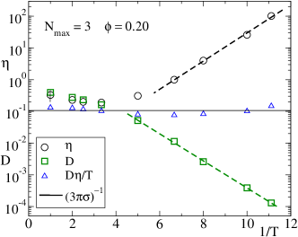
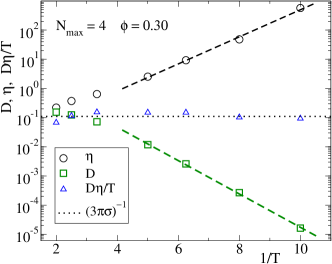
Figure 1: $T$ dependence of the diffusivity $D$, the viscosity $\eta$, and the product $D\eta/T$ for the cases $N_{\rm max}=3$, $\phi=0.20$ (top panel), and $N_{\rm max}=4$, $\phi=0.30$ (bottom panel). Dotted lines correspond to the expected value $(3\pi\sigma)^{-1}$ from the Stokes-Einstein relation. Dashed lines are fits to Arrhenius laws. An error bar is included for the viscosity at high $T$.

Long time decays of dynamic correlators in supercooled states are usually well described by the phenomenological Kohlrausch-Williams-Watts (KWW) function $\exp[-(t/\tau)^{\beta}]$, where $\tau$ is the corresponding relaxation time and $\beta$ is a stretching exponent which takes values $0<\beta<1$. Experimental evidence for a collection of chemically and structurally very different glass-forming liquids bohmer shows that the smaller the fragility index (i.e., the closer the system is to strictly strong behavior), the closer to unity the values of $\beta$ are. Figure 2 shows that this is indeed the case for the $N_{\rm max}$ model. The long-time dependence of the normalized coherent intermediate scattering function, $\phi_{q}(t)=\langle\rho_{q}(t)\rho_{-q}(0)\rangle/\langle\rho_{q}(0)\rho_{-q}(0)\rangle$, where $\rho_{q}(t)=\sum_{i=1}^{N}\exp[i{\bf q}\cdot{\bf r_{i}}(t)]$, can be well described by KWW fits with values of $\beta>0.85$ in all the $q$ range and for all studied $\phi$. Such a behavior is observed at all $T$ where the system shows Arrhenius behavior. As shown in Ref. bohmer , these $\beta$ values are very different from the ones typical of fragile liquids ($\beta\sim 0.5$).

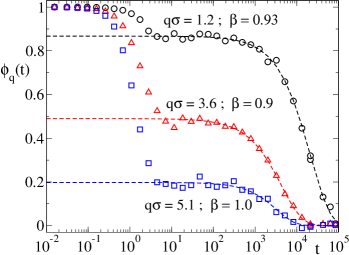
Figure 2: Symbols: Coherent intermediate scattering function for $N_{\rm max}=4$, $\phi=0.30$, and $T=0.1$, for different values of the wavevector $q$. Dashed lines are KWW fits. The stretching exponents $\beta$ are indicated for the corresponding $q$’s.

Results reported in Figs. 1 and 2 provide convincing evidence that Eqs. (1, 2) define a simple and satisfactory minimal model for a strong glass-forming liquid.

b) Energy landscape

Fig. 3 shows the $T$ dependence of the potential energy (i.e., the energy of the typical bonding pattern) per particle, $E$. In the present model, the potential energy of each configuration coincides with the energy of the bonding pattern and can be directly associated, in the Stillinger-Weber formalism, with the IS energy. Within the times accessible by the simulations, equilibrium states can be reached for configurations characterized by a number of broken bonds smaller than a 2 %, i.e. the lowest energy state, $E_{\rm fb}$, is approached from equilibrium simulations.

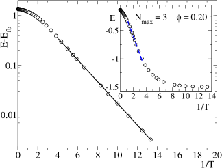
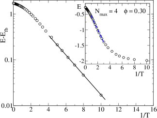
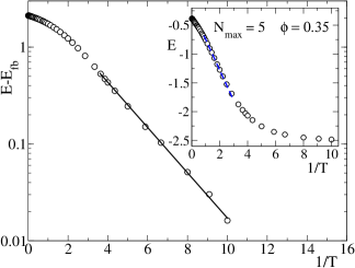
Figure 3: $T$ dependence of the potential energy per particle $E$ for the cases $N_{\rm max}=3$, $\phi=0.20$ (top panel), $N_{\rm max}=4$, $\phi=0.30$ (middle panel), and $N_{\rm max}=5$, $\phi=0.35$ (bottom panel). Full lines at low $T$ are fits to Arrhenius behavior with activation energy $u_{0}/2$ (see text and Table 1). Dashed lines at high $T$ correspond to linear behavior in $T^{-1}$ (see text).

From the low $T$ behavior of $E$, one sees that the approach to $E_{\rm fb}$ is well described by an Arrhenius law:

$$E-E_{\rm fb}=A_{\infty}^{\rm f}\exp(-\epsilon_{\rm f}/k_{\rm B}T).$$ (15)

The activation energy $\epsilon_{\rm f}$, determined by a free fit, is close to $u_{0}/2$. Indeed, by forcing the Arrhenius activation energy to be exactly $u_{0}/2$ a satisfactory representation of the data is recovered, with one simple fitting parameter $A_{\infty}$. Figure 3 shows the result of a fit to $E-E_{\rm fb}=A_{\infty}\exp(-u_{0}/2k_{\rm B}T)$. The corresponding best-fitting values, with two ($A^{\rm f}_{\infty},u_{0}$) and one ($A_{\infty}$) free parameters are reported in Table 1. The observed value $u_{0}/2$ is consistent with theoretical predictions based on the thermodynamic perturbation theory developed by Wertheim wertheim1 to study association in simple liquids. It is not a coincidence since in Wertheim’s theory bonds are also geometrically uncorrelated. Similar values are also predicted by more intuitive recent approaches sear .

	$(N_{\rm max},\phi)$		$A_{\infty}$		$A_{\infty}^{\rm f}$		$\epsilon_{\rm f}$
	(3, 0.20)		2.69		2.70		0.506
	(3, 0.30)		1.74		1.72		0.499
	(3, 0.35)		1.38		1.37		0.498
	(4, 0.30)		2.59		2.73		0.508
	(4, 0.35)		2.15		2.12		0.498
	(4, 0.40)		1.70		1.67		0.498
	(4, 0.45)		1.28		1.23		0.495
	(4, 0.50)		0.900		0.884		0.498
	(5, 0.35)		3.14		3.73		0.539

Table 1: Fit parameters for the low $T$ Arrhenius dependence of the potential energy $E$ (see text).

The clear low $T$ Arrhenius dependence and the explicit value of the activation energy provide a convenient way to evaluate the $T$ dependence of the energy for lower $T$. While in $T$, it might appear as a wide extrapolation procedure, we recall that in $E$ the interpolation extends only over a small (2%) range of energies, between the fully bonded state ($E=E_{\rm fb}$) and the lowest equilibrated state studied in simulations. Eq. (15) provides a convenient expression for the low $T$ behavior of $E$ and, by using Eq. (13), a way of calculating the total excess entropy down to the fully connected state.

We note on passing that at intermediate temperatures the $T$ dependence of $E$ is consistent with a $1/T$ law, as expected for a Gaussian distribution of energy levels. The $1/T$ law crosses to the Arrhenius dependence on cooling. This crossing has been also observed in the study of the $T$ dependence of the IS energy in a realistic (atomistic) model for silica voivod01 ; newheuer .

Figure 4: Full lines: $T$ dependence of the isochoric configurational specific heat for several values of ($N_{\rm max}$, $\phi$). Dashed lines are an extrapolation to high $T$ of the low $T$ behavior $A^{\rm f}_{\infty}\epsilon_{\rm f}k^{-1}_{\rm B}T^{-2}\exp(-\epsilon_{\rm f}/k_{\rm B}T)$ (see text).

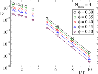
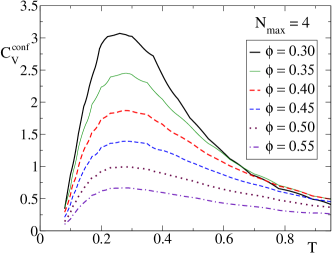
Figure 5: $T$ dependence of the diffusivity (top panel) and the isochoric configurational specific heat (bottom panel) for $N_{\rm max}=4$, at several values of $\phi$. Dashed lines in top panel are Arrhenius fits.

The low $T$ Arrhenius dependence of $E$ [Eq. (15)] has a practical implication in the $T$ dependence of the isochoric configurational specific heat $C_{V}^{\rm conf}(T)=(\partial E/\partial T)_{V}$. Hence, from Eq. (15), at low $T$ we have $C_{V}^{\rm conf}(T)=A^{\rm f}_{\infty}\epsilon_{\rm f}k^{-1}_{\rm B}T^{-2}\exp(-\epsilon_{\rm f}/k_{\rm B}T)$, which has a maximum at $T=\epsilon_{\rm f}/2\approx u_{0}/4$. Fig. 4 shows that indeed, numerical data for $C_{V}^{\rm conf}$ display a peak at $T\approx 0.25$. A peak in $C_{V}^{\rm conf}(T)$ has also been observed in recent simulations of atomistic models of two different network-forming liquids: silica voivod01 and BeF₂ hemmati .

We note that a strong correlation is observed between the $T$ dependence of the diffusivity and the $T$ dependence of the potential energy. Fig. 5 shows, for $N_{\rm max}=4$ and several $\phi$ values, that on cooling, $D$ crosses to an Arrhenius law at $T\approx 0.25$. This temperature is the same at which the specific heat shows a maximum. This correlation holds at all the investigated $\phi$ values.

The quality of the low $T$ Arrhenius fits for the diffusivities is worse at high $\phi$. Indeed, low $T$ data at high $\phi$ show some bending (Fig. 5a). This result suggests that the system will become more fragile with increasing density. This is not surprising, since the influence of the square well will be weaker at higher packing, and the system will approach a dense hard sphere liquid, which is a fragile system.

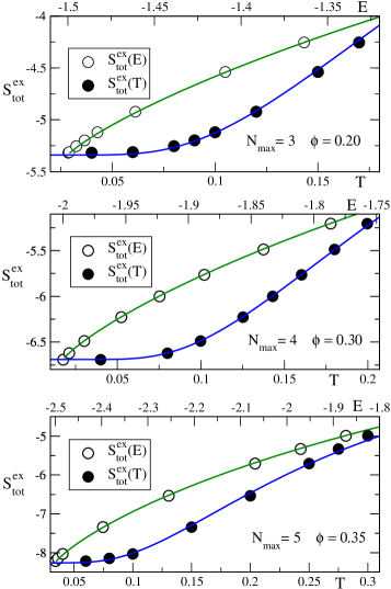
Figure 6: $E$ and $T$ dependence of the total excess entropy over the ideal gas value, $S^{\rm ex}_{\rm tot}$, for the cases $N_{\rm max}=3$, $\phi=0.20$ (top panel), $N_{\rm max}=4$, $\phi=0.30$ (middle panel), and $N_{\rm max}=5$, $\phi=0.35$ (bottom panel). Continuous lines for $S^{\rm ex}_{\rm tot}(E)$ are obtained as the sum of the fit functions for $S^{\rm ex}_{\rm vib}(E)$ [Eq. (16)] and $S_{\rm conf}(E)$ [Eq. (19)]. Continuous lines for $S^{\rm ex}_{\rm tot}(T)$ are parametrically obtained from the $T$ dependence of $E$.

Next we turn to the evaluation of the statistical properties of the PEL, and more precisely the total excess entropy and its vibrational and configurational contributions. As explained in Section III [Eq. (13)], the total excess entropy $S_{\rm tot}^{\rm ex}$ is evaluated by isochoric integration from the hard sphere limit at a sufficiently high $T_{\rm ref}$. We use a value $T_{\rm ref}=100$. Fig. 6 shows $S_{\rm tot}^{\rm ex}$ as a function of $T$ and $E$, for different values of $\phi$ and $N_{\max}$. Due to the presence of the interaction potential (1, 2), $S_{\rm tot}^{\rm ex}$ is negative (see also below). As expected, $S^{\rm ex}_{\rm tot}(T)$ decays to a constant value at low $T$, since the system is very close to the fully bonded state and no further structural changes are expected to occur. A glass transition temperature $T_{\rm g}$ can be operationally defined as the $T$ at which relaxation becomes longer than the simulation time. The fact that the system is so close to its lowest energy state already above this operational $T_{\rm g}$ implies that a very small drop of the specific heat is expected at $T_{\rm g}$, consistently with experimental evidence in strong liquids martinez .

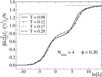
Figure 7: $\lambda$ dependence of $\beta\lambda\langle\sum_{i=1}^{N}({\bf r}_{i}-{\bf r}_{i}^{0})^{2}\rangle_{\lambda}/N$, for $N_{\rm max}=4$ and $\phi=0.30$, at different temperatures. The horizontal line indicates the expected value 3/2 for harmonic behavior.

The evaluation of the vibrational contribution $S_{\rm vib}^{\rm ex}$ [Eq. (11)] requires the calculation of the integral over the coupling constants $\lambda$. Fig. 7 shows the calculated $\lambda$ dependence of $\lambda\langle\sum_{i=1}^{N}({\bf r}_{i}-{\bf r}_{i}^{0})^{2}\rangle_{\lambda}/N$ at several $T$ for one specific value of $N_{\rm max}$ and $\phi$. Data for different $N_{\rm max}$ and $\phi$ display a similar behavior. At values $\lambda<\lambda_{\rm min}\approx 10^{-6}$ contributions to the integral in Eq. (11) are negligible, and $\lambda_{\rm min}$ is taken as lower-cut for integration. At large $\lambda$ values, $\lambda\langle\sum_{i=1}^{N}({\bf r}_{i}-{\bf r}_{i}^{0})^{2}\rangle_{\lambda}/N$ approaches the theoretical limit $3k_{\rm B}T/2$. This value is reached at $\lambda_{\rm max}\gtrsim 10^{6}$. Note that $\lambda=10^{6}$ corresponds to an average displacement per particle of the order of $10^{-4}$ for this $T$ range. Hence the harmonic perturbation localize the particles in a well much narrower than the square well width $\Delta$, so that the presence of the unperturbed potential is irrelevant for this upper $\lambda$ value.

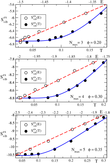
Figure 8: As Fig. 6 for the excess vibrational entropy, $S^{\rm ex}_{\rm vib}$. Dashed lines for $S^{\rm ex}_{\rm vib}(E)$ are linear fits [Eq. (16)]. Continuous lines for $S^{\rm ex}_{\rm vib}(T)$ are parametrically obtained from the $T$ dependence of $E$ (see text).

Fig. 8 shows the $T$ and $E$ dependence of $S_{\rm vib}^{\rm ex}$ for the same values of $\phi$ and $N_{\rm max}$ of Fig. 6. Close to the fully connected state $S_{\rm vib}^{\rm ex}$ can be well described by a linear dependence on the energy (i.e. on the number of bonds):

$$S^{\rm ex}_{\rm vib}(E)=S^{\rm ex}_{\rm vib}(E_{\rm fb})+\gamma_{\rm vib}(E-E_{\rm fb}).$$ (16)

Interestingly, this linear dependence on the basin depth has also been observed in previously investigated models of supercooled liquids sastry01 ; press ; mossaotp ; buchner1 ; wales .

Finally, the configurational entropy $S_{\rm conf}$ is determined as $S^{\rm ex}_{\rm tot}-S^{\rm ex}_{\rm vib}$. Fig. 9 shows $S_{\rm conf}$ for the same $\phi$ and $N_{\rm max}$ of Figs. 6 and 8. Some considerations are in order: as for the total entropy, $S_{\rm conf}$ approaches a constant value at low $T$. Interestingly enough, this constant value is significantly different from zero. The fully connected network is thus characterized by an extensive number of distinct bond configurations $\sim\exp(NS_{\rm conf})$. These different network configurations arise from different bond topologies, i.e., disorder is associated to the presence of closed loops of different number of bonds.

To derive a functional form for the $E$ dependence of $S_{\rm conf}$, we start from the thermodynamic relation $(\partial S/\partial E)_{V}=1/T$, which in the present case can be written as:

$$\frac{\partial(S_{\rm conf}+S_{\rm vib})}{\partial(E-E_{\rm fb})}=\frac{1}{T}.$$ (17)

At low $T$, from Eq. (15) we obtain $1/T=-(1/\epsilon_{\rm f})\ln[(E-E_{\rm fb})/A^{\rm f}_{\infty}]$ and, making use of Eq. (16) we find:

$$\frac{\partial S_{\rm conf}}{\partial(E-E_{\rm fb})}=-\gamma_{\rm vib}-\frac{1}{\epsilon_{\rm f}}\ln\frac{E-E_{\rm fb}}{A^{\rm f}_{\infty}},$$ (18)

which, after integration, provides the $E$ dependence of the configurational entropy:

$$S_{\rm conf}(E)=S_{\rm conf}(E_{\rm fb})$$

$$-\frac{E-E_{\rm fb}}{\epsilon_{\rm f}}\ln[2(E-E_{\rm fb})]+\gamma_{\rm conf}(E-E_{\rm fb}),$$ (19)

where the constant $\gamma_{\rm conf}$ is given by:

$$\gamma_{\rm conf}=\frac{1}{\epsilon_{\rm f}}-\gamma_{\rm vib}+\frac{\ln(2A^{\rm f}_{\infty})}{\epsilon_{\rm f}}.$$ (20)

As mentioned above, a satisfactory description of the low $T$ Arrhenius dependence of $E$ is provided by forcing a value $u_{0}/2$ for the activation energy $\epsilon_{\rm f}$. Hence, we can make the changes $\epsilon_{\rm f}\rightarrow u_{0}/2$ and $A^{\rm f}_{\infty}\rightarrow A_{\infty}$ in Eqs. (19, 20). These changes allow us to obtain a simple expression of $S_{\rm conf}$ in terms of the number of broken bonds. Hence, since $E-E_{\rm fb}=N_{\rm bb}u_{0}$, we find:

$$S_{\rm conf}(E)=S_{\rm conf}(E_{\rm fb})-2N_{\rm bb}\ln(2N_{\rm bb})+\gamma_{\rm conf}N_{\rm bb}.$$ (21)

This expression suggests that the low-$E,T$ dependence of the configurational entropy is controlled by a combinatorial factor related to the number of broken bonds randomly distributed along the network. The derivation also shows how intimately the logarithmic dependence of the entropy is connected to the Arrhenius dependence of $E$ at low $T$. The final expression for $S_{\rm conf}(E)$ is very different from the quadratic energy dependence resulting from the Gaussian distribution of IS energies observed in models of fragile liquids st ; sastry01 ; starr01 ; press .

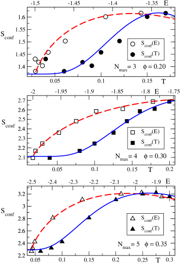
Figure 9: As Figs. 6 and 8 for the configurational entropy, $S_{\rm conf}$. Dashed lines for $S_{\rm conf}(E)$ are fits to Eq. (19). Continuous lines for $S_{\rm conf}(T)$ are parametrically obtained from the $T$ dependence of $E$ (see text). A typical error bar is shown in down panel.

To provide a further and analysis-free confirmation of the crossover at low $T$ toward combinatorial statistics of the bonding energy states, we show in Fig. 10 the $T$ dependence of $E$ for $N_{\rm max}=4$ at several $\phi$ values. We show a representation of $E-E_{\rm fb}$, both in linear and logarithmic scale, as a function of $1/T$. We note that, for all $\phi$, when $E-E_{\rm fb}\approx 0.75$ the $1/T$ law, which is expected to hold in a Gaussian landscape, breaks down. Similarly, when $E-E_{\rm fb}\approx 0.3$ the Arrhenius law sets in. The fact that both crossovers are, at most, weakly dependent on $\phi$ suggests that they are esentially controlled by the bonding statistics and that between $E-E_{\rm fb}\approx 0.75$ and $E-E_{\rm fb}\approx 0.3$ a crossover from Gaussian to logarithmic statistics occurs.

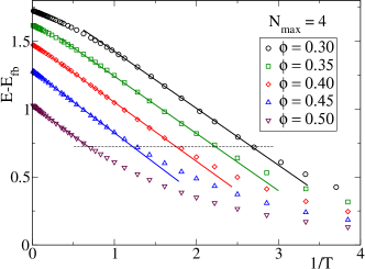
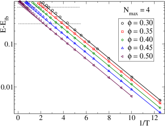
Figure 10: $T$ dependence of $E-E_{\rm fb}$ at different regions of the energy landscape. Top panel: Full lines correspond to behavior linear in $1/T$. The horizontal dashed line indicates the departure of such behavior. Bottom panel: Full lines correspond to Arrhenius behavior. The horizontal dashed lines indicate the limits of Arrhenius and $1/T$ behavior.

Fig. 9 shows the $E$ and $T$ dependence of $S_{\rm conf}$ for different values of $N_{\rm max}$. Eq. (19) provides a good description of the data. No fit parameters are involved in comparing the numerical estimates of $S_{\rm conf}$ and the predictions of Eq. (19) , except for the constant $S_{\rm conf}(E_{\rm fb})$. Note that $\gamma_{\rm conf}$ is not a fit parameter, but a function [Eq. (20)] of parameters defining $E(T)$ and $S^{\rm ex}_{\rm vib}(E)$. Before discussing the calculated values for $S_{\rm conf}(E_{\rm fb})$, we present in Fig. 11 the $E$ dependence of the configurational and excess vibrational entropies for $N_{\rm max}=4$ and different packing fractions $\phi$. For all $\phi$, the same functional forms of Eqs. (16) and (19) are recovered respectively for $S^{\rm ex}_{\rm vib}$ and $S_{\rm conf}$. The two quantities show an opposite trend. Curves for $S_{\rm conf}(E)$ tend to collapse at high $\phi$, while those for $S^{\rm ex}_{\rm vib}(E)$ tend to collapse at low $\phi$. Interestingly, the configurational entropy just shifts with varying $\phi$.

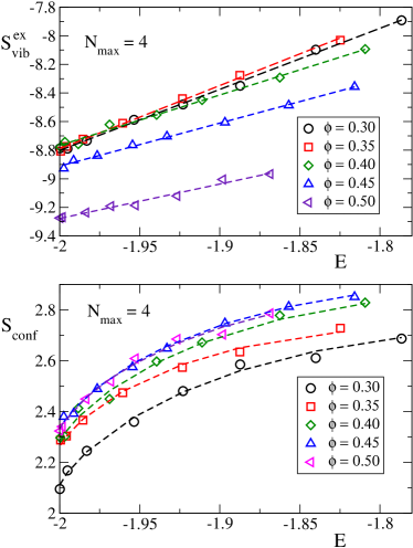
Figure 11: $E$ dependence of $S_{\rm vib}^{\rm ex}$ and $S_{\rm conf}$ for $N_{\rm max}=4$ and different values of $\phi$. Dashed lines in top and bottom panels are, respectively, fits to Eqs. (16) and (19).

Table 2 summarizes the results of the fits of the vibrational and configurational entropies to Eqs. (16) and (19) for the studied range of control parameters. Data shown in the table help discussing the $N_{\rm max}$ and $\phi$ dependence of the entropy of the fully bonded state. A trend in the direction of increasing $S_{\rm conf}(E_{\rm fb})$ on increasing $N_{\rm max}$ is observed very clearly in the comparison between $N_{\rm max}=3$ and $N_{\rm max}=4$. Much weaker is the trend between $N_{\rm max}=4$ and $N_{\rm max}=5$. A similar weak trend is observed for $N_{\rm max}=4$ on increasing $\phi$. The weak increase of $S_{\rm conf}(E_{\rm fb})$ with increasing $\phi$ suggests that when the system is compressed, neighboring particles progressively enter in the interaction range of a given one, yielding a major variety of local configurations of the bonding pattern, and consequently, more topologically distinct fully bonded networks. The trend of the excess vibrational entropy suggests that the available free volume for a given bonding pattern decreases with increasing $\phi$.

	$(N_{\rm max},\phi)$	$S_{\rm conf}(E_{\rm fb})$	$\gamma_{\rm conf}$	$S^{\rm ex}_{\rm vib}(E_{\rm fb})$	$\gamma_{\rm vib}$
	(3, 0.20)	1.37	-0.79	-6.71	6.16
	(3, 0.30)	1.55	-0.336	-6.60	4.83
	(3, 0.35)	1.63	-1.02	-6.70	5.05
	(4, 0.30)	2.11	1.02	-8.80	4.27
	(4, 0.35)	2.26	0.49	-8.79	4.43
	(4, 0.40)	2.28	0.93	-8.77	3.52
	(4, 0.45)	2.33	0.87	-8.91	3.01
	(4, 0.50)	2.33	0.77	-9.27	2.41
	(5, 0.35)	2.28	1.84	-10.55	3.83

Table 2: Parameters defining the configurational [Eq.(19)] and excess vibrational [Eq.(16)] entropy for the studied values of $N_{\rm max}$ and $\phi$.

A summary of the landscape analysis for all studied $\phi$ is shown in Fig. 12 for $N_{\rm max}=4$. The figure shows the $\phi$ dependence of $S_{\rm tot}^{\rm ex}$, $S_{\rm vib}^{\rm ex}$ and $S_{\rm conf}$ for several different low $T$ isotherms, all in the Arrhenius region of energies. It clearly emerges that the significant reduction of $S_{\rm tot}^{\rm ex}$ on increasing $\phi$ arises essentially from the vibrational component. We also note that the HS relative contribution to $S_{\rm tot}^{\rm ex}$ increases on increasing $\phi$. Hence, according to Eq. (12), $S^{\rm ex}_{\rm HS}(\phi=0.30)=-1.90$, while $S^{\rm ex}_{\rm HS}(\phi=0.50)=-5.0$. By comparing with data in Fig. 12, it is clear that $S_{\rm tot}^{\rm ex}$ is dominated by the square-well and hard-sphere contributions at respectively low and high packing fraction.

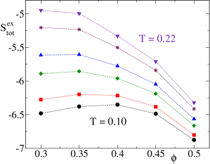
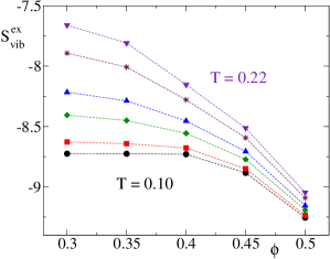
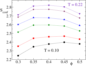
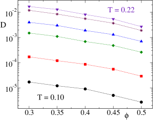
Figure 12: $\phi$ dependence of $S^{\rm ex}_{\rm tot}$, $S^{\rm ex}_{\rm vib}$, $S_{\rm conf}$, and $D$, for $N_{\rm max}=4$ along isothermal curves. In all figures, from top to bottom, the isothermals are $T=$ 0.22, 0.20, 0.17, 0.15, 0.12 and 0.10. Dashed lines are guides for the eyes.

It is also interesting to observe that, within the precision of the data, $S_{\rm conf}$ shows a weak maximum, shifting to higher $\phi$ on cooling. To test wether the presence of a maximum of $S_{\rm conf}$ has some effect on the dynamics we also show in Fig. 12 the behavior of the diffusivity along the same isotherms. We note that $D$ is monotonic in $\phi$ and hence that the maximum in the configurational entropy does not provoke a maximum in the diffusivity. We also note that an isochoric plot (not shown) of $\log D$ vs. $[TS_{\rm conf}(T)]^{-1}$ provides a satisfactory linearization of the data, as suggested by the Adam-Gibbs theory adamgibbs . This is not inconsistent with the observed Arrhenius dependence of $D$, since the $T$ dependence of $S_{\rm conf}(T)$ is only at most 20% of $S_{\rm conf}(E_{\rm fb})$.

V. CONCLUSIONS

This article reports an explicit numerical calculation of the potential energy landscape for a simple model of strong liquids. It shows that it is possible to calculate with arbitrary precision the statistical properties of the landscape relevant to the behavior of the system at low $T$, when all particles are connected by bonds. The model can be seen as a zero-th order model for network-forming liquids, capturing the limited valency of the interaction and the open structure of the liquid. By construction, it misses all geometric correlations between different bonds which are present in network-forming materials. The simplicity of the model has several advantages, some of which of fundamental importance for an exact evaluation of the landscape properties. Hence, since angular constraints between bonds are missing, it is possible to equilibrate the system to very low $T$, reaching configurations which are essentially fully bonded. At the lowest studied $T$, less than 2% of the bonds are broken in average. Differently from other studied models with fixed bonding site geometries kolafa ; vega ; demichele , the absence of geometric constraints makes it possible to reach almost fully bonded states in a wide range of densities. Moreover, the use of a square well interaction as bonding potential has the advantage that the energy of the fully bonded state (the lowest possible energy) is known.

The present model neglects completely interactions between particles which are not nearest neighbors. The energy of a particle is indeed fully controlled by the bonds with the nearby particles. This element of the model favors a sharp definition of the energy and a clear-cut definition of basins. On the other hand, in network-forming liquids, bonding is often of electrostatic origin and interactions are not limited to the first shell of neighbors. This produces a much wider variety of local environments and, as a consequence, a spreading of the energy levels. These residual interactions, if smaller than the bonding interactions, will only contribute to spread the distribution of energy states without changing the landscape features (down to $T$ of the order of the energy spreading).

The use of square-well interactions has a major advantage in relation to the possibility of precisely calculating landscape properties, since the energy of the system becomes a measure of the number of bonds. A basin in configuration space can be identified as a bonding pattern, and a transition between different basins becomes associated to bond forming and breaking. Under these conditions, the basin boundaries are properly defined. We have shown that the method of the Perturbed Hamiltonian can be extended to the present model, providing a formally exact method to evaluate the vibrational component of the free energy. This is a relevant achievement, since the evaluation of the vibrational entropy is the only weak point in all estimates of landscape properties in models with continuous potentials jstat ; angelanientro . Indeed, when the potential is continuous, the constraint of exploring a fixed basin can not be implemented unambiguously in the Frenkel-Ladd method due to the difficulty of detecting crossing between different basins. Such a difficulty is not present in the square-well potential, since crossing of a basin is detected by a finite energy change.

The two relevant features observed in this study are: (i) A residual value of the configurational entropy for $T\rightarrow 0$, associated to the exponentially large number of distinct fully connected bonding patterns. (ii) A logarithmic dependence of the number of bonding patterns on the number of broken bonds [Eq. (21)]. These two features are common to all investigated values of $N_{\rm max}$ and to all studied $\phi$. A consequence of the logarithmic landscape statistics is the absence of a finite temperature at with the lowest energy state is reached loglands . Indeed from Eq. (19) it is found that $\partial S/\partial E|_{E=E_{\rm fb}}=\infty$, and hence $E_{\rm fb}$ is reached only at $T=0$.

According to the picture emerging from this study, strong liquid behavior is connected to the existence of an energy scale, provided by the bond energy, which is discrete and dominant as compared to the energetic contributions coming from non-bonded next-nearest neighbor interactions angellbond . It is also intimately connected to the existence of a significantly degenerate lowest energy state, favoring the formation of highly bonded states which can still entropically rearrange to form different bonding patterns with the same energy. Of course, the specific value of $S_{\rm conf}(E_{\rm fb})$ in the $N_{\rm max}$ model provides an upper bound to the value expected in network-forming liquids sceats ; rivier , since the absence of angular constraints significantly increases the number of geometric arrangements of the particles compatible with a fully bonded state. Recent estimates in glassy water speedywatexp , which forms a tetrahedral disordered network, suggest a residual value of the configurational entropy of the order of $\approx 0.3k_{\rm B}$ . Hence the localization of the bonding sites at specific locations, and the associated geometrical correlations, do produce a significant reduction of $S_{\rm conf}(E_{\rm fb})$.

Results reported in this article suggest that strong and fragile liquids are characterized by significant differences in their potential energy landscape properties. A non-degenerate disordered lowest energy state and Gaussian statistics characterize fragile liquids, while a degenerate disordered lowest energy state and logarithmic statistics are associated with strong liquids. These results rationalize previous landscape analysis of realistic models of network-forming liquids voivod01 , and the recent observation by Heuer and coworkers that the breakdown of Gaussian landscape statistics is associated with the formation of a connected network newheuer . While in atomistic models the lowest energy state is not known, and the very long equilibration times prevent an unambiguous determination of its degeneracy, both these quantities are accessible in the present simple model.

A last remark concerns the limit of the $N_{\rm max}$ value for which the fully connected state can be reached. The possibility of approaching the fully bonded state is limited by the possibility of avoiding the $(T-\phi)$ region where liquid-gas phase separation is present. It has recently been observed gel ; gellong ; gelgenova that the region of unstable states expands on increasing $N_{\rm max}$ and essentially covers, at low $T$, the entire accessible $\phi$ range when $N_{\rm max}\geq 6$. For these large $N_{\rm max}$ values, slowing down of the dynamics is observed only at very large $\phi$ and it is essentially controlled by packing considerations, not by bonding. In this respect, bond-controlled dynamics are observable only when the valence of the interparticle interaction is limited.

ACKNOWLEDGEMENTS

We thank K. Binder, A. Heuer, C. De Michele, P. H. Poole, A. M. Puertas, S. Sastry, R. Schilling, N. Wagner and F. Zamponi for useful discussions and critical readings of the manuscript. MIUR-COFIN and MIUR-FIRB are acknowledged for financial support. Additional support is also acknowledged from NSF (S. V. B.) and NSERC-Canada (I. S.-V.).

References

- (1) P. G. Debenedetti, Metastable liquids. Concept and principles, Princeton University Press, Princeton, New Jersey (1996).
- (2) K. Binder and W. Kob, Glassy materials and disordered solids. An introduction to their Statistical Mechanics, World Scientific (2005).
- (3) C. A. Angell, J. Non-Cryst. Solids 73, 1 (1985).
- (4) R. Böhmer, K. L. Ngai, C. A. Angell and D. J. Plazek, J. Chem. Phys. 99, 4201 (1993).
- (5) L. M. Martínez and C. A. Angell, Nature 410, 663 (2001).
- (6) H. Vogel, Z. Phys. 22, 645 (1921); G. S. Fulcher, J. Am. Ceram. Soc. 8, 339 (1923); G. Tammann and W. Hesse, Z. Anorg. Allg. Chem. 156, 245 (1926).
- (7) W. Kauzmann, Chem. Rev. 43, 219 (1948).
- (8) Some polymers of complex architecture display notable differences between and . See Ref. cangialosi for a recent discussion on the possible origin of this discrepancy.
- (9) D. Cangialosi, A. Alegría, and J. Colmenero, Europhys. Lett. 70, 614 (2005).
- (10) A. Cavagna, I. Giardina, and T. S. Grigera, Europhys. Lett. 61, 74 (2003); J. Chem. Phys. 118, 6974 (2003).
- (11) F.H. Stillinger, J. Chem. Phys. 88, 7818 (1988).
- (12) J. H. Gibbs and E. A. DiMarzio, J. Chem. Phys. 28, 373 (1958).
- (13) B. Derrida, Phys. Rev. B 24, 2613 (1981); T. Keyes, J. Chowdhary, and J. Kim, Phys. Rev. E 66, 051110 (2002); M. Sasai, J. Chem. Phys. 118 (2003).
- (14) T. R. Kirkpatrick and P. G. Wolynes, Phys. Rev. B 36, 8552 (1987).
- (15) M. Mezard and G. Parisi, Phys. Rev. Lett. 82, 747 (1999).
- (16) M. Goldstein, J. Chem. Phys. 51, 3728 (1969).
- (17) F. H. Stillinger and T. A. Weber, Phys. Rev. A 25, 978 (1982).
- (18) F. H. Stillinger and T. A. Weber, Science 225, 983 (1984); F. H. Stillinger, ibid. 267, 1935 (1995).
- (19) D. Wales, Energy Landscapes, Cambridge University Press, Cambridge (2004).
- (20) C. A. Angell, Science 267, 1924 (1995).
- (21) F. Sciortino, J. Stat. Mech., P05015 (2005).
- (22) S. Sastry, P. G. Debenedetti, and F. H. Stillinger, Nature 393, 554 (1998).
- (23) F. Sciortino, W. Kob, and P. Tartaglia, Phys. Rev. Lett. 83, 3214 (1999).
- (24) S. Büchner and A. Heuer, Phys. Rev. E 60, 6507 (1999).
- (25) L. Angelani, R. Di Leonardo, G. Ruocco, A. Scala, and F. Sciortino, Phys. Rev. Lett. 85, 5356 (2000).
- (26) T. S. Grigera, A. Cavagna, I. Giardina, and G. Parisi, Phys. Rev. Lett. 88, 055502 (2002).
- (27) A. Scala, F. W. Starr, E. La Nave, F. Sciortino, and H. E. Stanley, Nature 406, 166 (2000).
- (28) F. Sciortino and P. Tartaglia, Phys. Rev. Lett. 86, 107 (2001).
- (29) S. Sastry, Nature 409, 164 (2001).
- (30) P. G. Debenedetti and F. H. Stillinger, Nature 410, 259 (2001).
- (31) I. Saika-Voivod, P. H. Poole, and F. Sciortino, Nature 412, 514 (2001); Phys. Rev. E 69, 041503 (2004).
- (32) T. F. Middleton and D. J. Wales, Phys. Rev. B 64, 024205 (2001).
- (33) E. La Nave, A. Scala, F. W. Starr, H. E. Stanley, and F. Sciortino, Phys. Rev. E 64, 036102 (2001).
- (34) F. W. Starr, S. Sastry, E. La Nave, A. Scala, H. E. Stanley, and F. Sciortino, Phys. Rev. E 63, 041201 (2001).
- (35) E. La Nave, S. Mossa, and F. Sciortino, Phys. Rev. Lett. 88, 225701 (2002).
- (36) S. Mossa, E. La Nave, H. E. Stanley, C. Donati, F. Sciortino, and P. Tartaglia, Phys. Rev. E 65, 041205 (2002).
- (37) T. Keyes and J. Chowdhary, Phys. Rev. E 65, 041106 (2002).
- (38) G. Fabricius and D. A. Stariolo, Phys. Rev E 66, 031501 (2002).
- (39) L. Angelani, G. Ruocco, M. Sampoli, and F. Sciortino, J. Chem. Phys. 119, 2120 (2003).
- (40) B. Doliwa and A. Heuer, Phys. Rev. Lett. 23, 235501 (2003); Phys. Rev. E 67, 030501 (2003), ibid. 67, 031506 (2003).
- (41) M. Vogel, B. Doliwa, A. Heuer, and S. C. Glotzer, J. Chem. Phys. 120, 4404 (2004).
- (42) R. A. Denny, D. Reichman, and J. P. Bouchaud, Phys. Rev. Lett. 90, 025503 (2003).
- (43) A. Saksaengwijit, J. Reinisch, and A. Heuer, Phys. Rev. Lett. 93, 235701 (2004).
- (44) G. Ruocco, F. Sciortino, F. Zamponi, C. De Michele, and T. Scopigno, J. Chem. Phys. 120, 10666 (2004).
- (45) L. Angelani, G. Foffi, F. Sciortino, and P. Tartaglia, J. Phys.: Condens. Matter 17, L113 (2005).
- (46) A. Attili, P. Gallo, and M. Rovere, Phys. Rev. E 71, 031204 (2005).
- (47) A. Heuer and S. Büchner, J. Phys.: Condens. Matter 12, 6535 (2000).
- (48) A. J. Moreno, S. V. Buldyrev, E. La Nave, I. Saika-Voivod, F. Sciortino, P. Tartaglia, and E. Zaccarelli, Phys. Rev. Lett. 95, 157802 (2005).
- (49) R. J. Speedy and P. G. Debenedetti, Mol. Phys. 81, 237 (1994); ibid. 86, 1375 (1995); 88, 1293 (1996).
- (50) Y. Duda, C. J. Segura, E. Vakarin, M. F. Holovko, and W. G. Chapman, J. Chem. Phys. 108, 9168 (1998).
- (51) A. Huerta and G. G. Naumis, Phys. Rev. B 66, 184204 (2002).
- (52) E. Zaccarelli, S. V. Buldyrev, E. La Nave, A. J. Moreno, I. Saika-Voivod, F. Sciortino, and P. Tartaglia, Phys. Rev. Lett. 94, 218301 (2005).
- (53) E. Zaccarelli, I. Saika-Voivod, S. V. Buldyrev, A. J. Moreno, P. Tartaglia, and F. Sciortino, J. Chem. Phys. 124, 124908 (2006).
- (54) F. Sciortino, S. V. Buldyrev, C. De Michele, G. Foffi, N. Ghofraniha, E. La Nave, A. Moreno, S. Mossa, I. Saika-Voivod, P. Tartaglia, and E. Zaccarelli, Comp. Phys. Comm. 169, 166 (2005).
- (55) D. C. Rapaport. The Art of Molecular Dynamics Simulation, Cambridge University Press, Cambridge, UK., (1995).
- (56) This approximation for the anharmonic contribution works well in the case of soft potentials as Lennard-Jones 12-6 mossaotp , SPC/E water scala , or BKS silica voivod01 . However, it breaks down in the case of short-range steep potentials angelanientro as that of the model investigated in this work.
- (57) D. Frenkel and A.J.C. Ladd, J. Chem. Phys. 81, 3188 (1984).
- (58) D. Frenkel and B. Smit, Understanding Molecular Simulation, Academic Press, San Diego (1996).
- (59) B. Coluzzi, M. Mezard, G. Parisi, and P. Verrocchio, J. Chem. Phys. 111, 9039 (1999).
- (60) N. F. Carnahan and K. E. Starling, J. Chem. Phys. 51, 635 (1969).
- (61) B. J. Alder, D. M. Gass, and T. E. Wainwright, J. Chem. Phys. 53, 3813 (1970).
- (62) J. P. Hansen and I. M. McDonald, Theory of Simple Liquids, Academic Press, New York (1994).
- (63) M. S. Wertheim, J. Stat. Phys. 35, 19 (1984); ibid. 35, 35 (1984).
- (64) R. P. Sear and G. Jackson, J. Chem. Phys. 105, 1113 (1996).
- (65) M. Hemmati, C. T. Moynihan, and C. A. Angell, J. Chem. Phys. 115, 6663 (2001).
- (66) G. Adam and J. H. Gibbs, J. Chem. Phys. 43, 139 (1965).
- (67) J. Kolafa and I. Nezbeda, Mol. Phys. 61, 161 (1987).
- (68) C. Vega and P. A. Monson, J. Chem. Phys. 109, 9938 (1998).
- (69) C. De Michele, S. Gabrielli, F. Sciortino, and P. Tartaglia, cond-mat/0510787.
- (70) P. G. Debenedetti, F. H. Stillinger, and M. S. Shell, J. Phys. Chem B 107, 14434 (2003).
- (71) C. A. Angell and K. J. Rao, J. Chem. Phys. 57, 440 (1972).
- (72) M. G. Sceats, M. Stavola, and S. A. Rice, J. Chem. Phys. 70, 3927 (1979).
- (73) N. Rivier and F. Wooten, MATCH: Comm. Mat. Comp. Chem 48, 145 (2003).
- (74) R. J. Speedy, P. G. Debenedetti, R. S. Smith, C. Huang, and B. D. Kay, J. Chem. Phys. 105, 240 (1996).