Casimir interaction between a plate and a cylinder

Abstract

We find the exact Casimir force between a plate and a cylinder, a geometry intermediate between parallel plates, where the force is known exactly, and the plate–sphere, where it is known at large separations. The force has an unexpectedly weak decay $\sim L/(H^{3}\ln(H/R))$ at large plate–cylinder separations $H$ ($L$ and $R$ are the cylinder length and radius), due to transverse magnetic modes. Path integral quantization with a partial wave expansion additionally gives a qualitative difference for the density of states of electric and magnetic modes, and corrections at finite temperatures.

With recent advances in the fabrication of electronic and mechanical systems on the nanometer scale quantum effects like Casimir forces have become increasingly importantCleland+96 ; CAKBC2001 . These systems can probe mechanical oscillation modes of quasi one-dimensional structures such as nano wires or carbon nanotubes with high precision Sazonova+04 . However, thorough theoretical investigations of Casimir forces are to date limited to “closed” geometries such as parallel plates Casimir48 or, recently, a rectilinear “piston” hjks , where the zero point fluctuations are not diffracted into regions which are inaccessible to classical rays. A notable exception is the original work by Casimir and Polder on the interaction between a plate and an atom (sphere) at asymptotically large separation Casimir+48 .

In this Letter we consider the electrodynamic Casimir interaction between a plate and a parallel cylinder (or “wire”), both assumed to be perfect metals (see inset of Fig. 1). We show that the Casimir interaction can be computed without approximation for this geometry. We believe that the methods presented here may yield exact solutions for other interesting geometries as well. This geometry is also of recent experimental interest: Keeping two plates parallel has proved very difficult. The sphere and plate configuration avoids this problem, but the force is not extensive. The cylinder is easier to hold parallel and the force is extensive in its length Brown+05 .

Casimir interactions, while attractive for perfect metals in all known cases, depend strongly on geometry. Consider the Casimir interaction energy (discarding separation independent terms) at asymptotically large $H$ for three fundamental geometries which differ in the co-dimension of the surfacesScardicchio05 : two plates, plate–cylinder, and finally, plate–sphere, corresponding to co-dimension 1, 2, and 3, respectively. It is instructive to consider both a scalar field which vanishes on the surfaces (D $\equiv$ Dirichlet) and the electromagnetic field (EM). For parallel plates (area $A$) $E\sim\hbar cA/H^{3}$ in both cases Casimir48 . For a plate and a sphere of radius $R$, $E\sim\hbar cR/H^{2}$ Bulgac+05 for the Dirichlet case, as compared with $E\sim\hbar cR^{3}/H^{4}$ for the EM case Casimir+48 . Based on these results, expectations for the plate and cylinder geometry might range from $\sim\hbar cLR^{2}/H^{4}$, proportional to the cylinder volume, to $\sim\hbar cLR/H^{3}$, proportional to its surface area, or even $\sim\hbar cL/H^{2}$ with a potential non-power law dependence on the radius.

A simple but uncontrolled method for study of non-planar geometries is the proximity force approximation (PFA), where the system is treated as a sum of infinitesmal parallel plates Bordag+01 . Applied to the plate–cylinder geometry, the PFA yields $E_{\rm PFA}=-\frac{1}{960}\pi^{3}\hbar cL\sqrt{R/2a^{5}}$ to leading order in $a/R$, where $a=H-R$. Other approximations include semi-classical methods based on the Gutzwiller trace formula Schaden+00 , and a recent optical approach which sums also over closed but non-periodic pathsJaffe+04 . For large separations, a multiple scattering approach is available Balian , but has not been adapted to this geometry. For the Dirichlet case, a Monte Carlo approach based on worldline techniques has been applied to the plate-cylinder case Gies+03 .

Our result provides a test for the validity of these approximate schemes, and also provides insight into the large distance limit. In particular, we find the unexpected result that the electrodynamic Casimir force for the plate–cylinder geometry has the weakest of the possible decays,

$$F=-\frac{1}{8\pi}\frac{\hbar cL}{H^{3}\ln(H/R)}\,,$$ (1)

as $H/R\to\infty$. The same asymptotic result applies to a scalar field with Dirichlet boundary conditions. Interestingly, the decay exponent of the force is not monotonic in the number of co-dimensions: ($-4$, $-3-\epsilon$, $-5$) for co-dimension (1,2,3) respectively. In contrast the Dirichlet case is monotonic with exponents ($-4$,$-3-\epsilon$, $-3$).

In the remainder we derive these results, summarized in Eqs. (5)-(8), using path integral techniques. Our approach also yields the distance dependent part of the density of states, which contains the complete geometry dependent information of the photon spectrum, and is useful for computing thermal contributions to the force.

The translational symmetry along the cylinder axis enables a decomposition of the EM field into transverse magnetic (TM) and electric (TE) modes Emig+01 which are described by a scalar field obeying Dirichlet (D) or Neumann (N) boundary conditions respectively. We can compare our TM results to recent Monte Carlo Dirichlet results Gies+03 . Moreover, the mode decomposition turns out to be useful also in identifying the physical mechanism behind the weak decay of the force, which at large distance is fully dominated by D modes.

Our starting point is a path integral representation LK91 for the effective action which yields a trace formula for the density of states (DOS) Buscher+05 . The latter is then evaluated using a partial wave expansion. The DOS on the imaginary frequency axis is related to a Green’s function by $\rho(iq_{0})=(2q_{0}/\pi)\int d^{3}{\bf x}\,G({\bf x},{\bf x};q_{0})$, where $G({\bf x},{\bf x}^{\prime};q_{0})$ is the Green’s function for the scalar field with action $S=\frac{1}{2}\int d^{3}x(|\nabla\Phi|^{2}+(q^{0})^{2}\Phi^{2})$. The effect of boundaries on the Green function can be obtained by placing functional delta functions on the boundary surfaces in the functional integralLK91 . By integrating out both the field $\Phi$ and the auxiliary fields which represent the delta functions on the surfaces, one obtains the trace formula Buscher+05

$$\delta\rho(q_{0})=-\frac{1}{\pi}\frac{\partial}{\partial q_{0}}{\rm Tr}\ln\left(MM_{\infty}^{-1}\right)\,,$$ (2)

where $\delta\rho(q_{0})$ is the change in the DOS caused by moving the plate and cylinder in from infinity. The information about geometry is contained in the matrix $M$ of the quadratic action for the auxiliary fields, given by $M_{\alpha\beta}({\bf u},{\bf u}^{\prime};q_{0})=G_{0}({\bf s}_{\alpha}({\bf u})-{\bf s}_{\beta}({\bf u}^{\prime});q_{0})$ for D and by $M_{\alpha\beta}({\bf u},{\bf u}^{\prime};q_{0})=\partial_{{\bf n}_{\alpha}({\bf u})}\partial_{{\bf n}_{\beta}({\bf u}^{\prime})}G_{0}({\bf s}_{\alpha}({\bf u})-{\bf s}_{\beta}({\bf u}^{\prime});q_{0})$ for N boundary conditions; $G_{0}=e^{-q_{0}|{\bf x}|}/4\pi|{\bf x}|$ is the free space Green function, $\partial_{{\bf n}_{\alpha}}$ is its derivative normal to the surface, and ${\bf s}_{\alpha}({\bf u})$ parametrizes the surfaces (which are numbered by $\alpha=1$, $2$) in terms of surface coordinates ${\bf u}$. $M_{\infty}^{-1}$ is the functional inverse of $M$ at infinite surface separation. The trace in Eq. (2) runs over ${\bf u}$ and $\alpha$. For the cylinder with its axis oriented along the $x_{1}$ direction we set ${\bf s}_{1}(x_{1},\varphi)=(x_{1},R\sin(\varphi),R\cos(\varphi))$ and for the plate ${\bf s}_{2}(x_{1},x_{2})=(x_{1},x_{2},H)$ (see inset of Fig. 1).

The Casimir energy of interaction is given by $E=(\hbar c/2)\int_{0}^{\infty}dq_{0}q_{0}\delta\rho(q_{0})$. After transforming to momentum space, $\tilde{M}$, the Fourier transform of the matrix $M$ has block diagonal form with respect to $q_{0}$ and the momentum $q_{1}$ along the cylinder axis, so the Casimir energy can be expressed as,

$$E=\frac{\hbar cL}{8\pi^{2}}\int\!\!\!\int dq_{0}dq_{1}\ln\frac{\det\tilde{M}(q_{0},q_{1})}{\det\tilde{M}_{\infty}(q_{0},q_{1})}\,.$$ (3)

The elements of the matrix $M$ are labeled by the integer index $m=-\infty,\ldots,\infty$ coming from the compact $\varphi$-dimension of the cylinder, and the momentum $q_{2}$ along the other direction parallel to the plate, to read

$$\tilde{M}=\left(\begin{array}[]{cc}A_{[m,m^{\prime}]}&B_{[m,q_{2}^{\prime}]}\\ B^{T}_{[q_{2},m^{\prime}]}&C_{[q_{2},q_{2}^{\prime}]}\end{array}\right).$$ (4)

The matrix $A_{[m,m^{\prime}]}$ is diagonal, with elements $A_{[m,m]}\equiv A_{m}=I_{m}(ru)K_{m}(ru)$ for D and $A_{m}=(u/H)^{2}I^{\prime}_{m}(ru)K^{\prime}_{m}(ru)$ for N modes. The matrix $C$ also has only diagonal elements $C_{[q_{2},q_{2}]}\equiv C(q_{2})=H/(2\sqrt{u^{2}+u_{2}^{2}})$ for D and $C(q_{2})=-\sqrt{u^{2}+u_{2}^{2}}/(2H)$ for N modes. The off-diagonal matrix $B$ is non-diagonal with $B_{[m,q_{2}]}\equiv B_{m}(q_{2})=\pi He^{-\sqrt{u^{2}+u_{2}^{2}}}I_{m}(ru)[u/(u_{2}+\sqrt{u^{2}+u_{2}^{2}})]^{m}/\sqrt{u^{2}+u_{2}^{2}}$ for D and $B_{m}(q_{2})=(\pi u/H)e^{-\sqrt{u^{2}+u_{2}^{2}}}I^{\prime}_{m}(ru)[u/(u_{2}+\sqrt{u^{2}+u_{2}^{2}})]^{-m}$ for N modes. Here, we have defined the dimensionless combinations $u=H\sqrt{q_{0}^{2}+q_{1}^{2}}$, $u_{2}=Hq_{2}$ and $r=R/H$. The determinant can be obtained straightforwardly, and the total energy can be decomposed to the sum of D and N mode contributions, as

$$E=-\frac{\hbar cL}{H^{2}}\left[\Phi^{D}(r)+\Phi^{N}(r)\right],$$ (5)

with

$$\Phi^{X}(r)=-\frac{1}{4\pi}\int_{0}^{\infty}du\,u\ln\left[\det(\mathbbm{1}-N^{X}(u,r))\right]\,.$$ (6)

The matrix $N^{X}(u)$ is given in terms of Bessel functions,

$$N^{D}_{\mu\nu}(u,r)=\frac{I_{\nu}(ru)}{K_{\mu}(ru)}K_{\mu+\nu}(2u),$$ (7)

for D modes and

$$N^{N}_{\mu\nu}(u,r)=-\frac{I^{\prime}_{\nu}(ru)}{K^{\prime}_{\mu}(ru)}K_{\mu+\nu}(2u),$$ (8)

for N modes. The determinant in Eq. (6) is taken with respect to the integer indices $\mu$, $\nu=-\infty,\ldots,\infty$. If the matrix $N^{X}$ is restricted to dimension $(2l+1)$ with $N_{00}^{X}$ as the central element, it then describes the contribution from $l$ partial waves, beginning with $s$-waves for $l=0$.

From Eq. (6), one can easily extract the asymptotic large distance behavior of the energy for $r=R/H\ll 1$. For Dirichlet modes s-waves dominate, while for Neumann modes both $s$- and $p$-waves ($l=1$) contribute at leading order in $r$. The two cases differ qualitatively, with

$$\Phi^{D}(r)=-\frac{1}{16\pi}\frac{1}{\ln r},\quad{\rm and}\quad\Phi^{N}(r)=\frac{5}{32\pi}r^{2}.$$ (9)

For $H\gg R$ the EM Casimir interaction is dominated by the D (TM) modes. Note that a naive application of the PFA for small $r$, where it is not justified, yields the incorrect scalings $\Phi^{D}(r)=\Phi^{N}(r)\sim r$.

The natural expectation from the Casimir–Polder result for the plate-sphere interaction, that the force at large distance is proportional to the volume of the cylinder, is incorrect. The physical reason for this difference is explained by considering spontaneous charge fluctuations. On a sphere, the positive and negative charges can be separated by at most distances of order $R\ll H$. The retarded van der Waals interactions between these dipoles and their images on the plate leads to the Casimir–Polder interaction Casimir+48 . In the cylinder, fluctuations of charge along the axis of the cylinder can create arbitrary large positively (or negatively) charged regions. The retarded interaction of these charges (not dipoles) with their images gives the dominant term of the Casimir force. This interpretation is consistent with the difference between the two types of modes, since for N modes such charge modulations cannot occur due to the absence of an electric field along the cylinder axis. Eventually, for a finite cylinder, in the very far region $H\gg L$, the charge fluctuations can be considered again as small dipoles, and the Casimir–Polder law is expected to reappear, making the force proportional to the volume of the cylinder $LR^{2}$.

We next consider arbitrary separations, and use Eq. (6) to obtain the contribution from higher order partial waves. A numerical evaluation of the determinant is straightforward, and we find that down to even small separations of $a/R=0.1$ the energy converges at order $l=25$, whereas for $a/R\gtrsim 1$ convergence is achieved for $l=4$. Fig. 1 shows our results for Dirichlet and Neumann modes and for their sum which is the EM Casimir energy, all scaled by the corresponding $E_{\rm PFA}$ given above foot1 . Both types of modes show a strong deviation from the PFA for $a/R\gtrsim 1$, especially the Dirichlet energy. Fig. 1 shows also very recent wordline-based Monte Carlo results for the Dirichlet case at moderate separations Gies-priv , which agree nicely with our exact results.

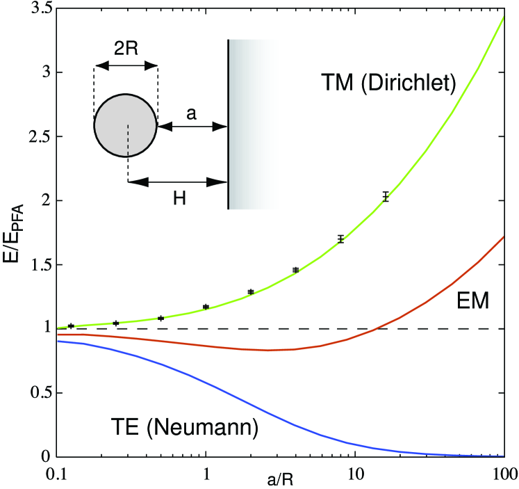
Figure 1: Ratio of the exact Casimir energy to the PFA for the geometry shown in the inset. All curves are obtained at order $25$ of the partial wave expansion, and the accuracy lies within the line thickness even at small $a/R$. The Dirichlet data points are from Ref. Gies-priv .

Eq. (9) indicates that the Dirichlet dominated force vanishes logarithmically as $R\to 0$ at fixed $H$. A similar result is obtained when the cylinder is replaced by an infinitesimal thin wire, but an UV cutoff is introduced to control short wavelength modes. Both results are a consequence of the fact that the asymptotic form of Eq. (9) is independent of the actual shape of the cross section of the wire, and the cutoff $R$ can be identified with any typical scale of the cross section. The leading asymptotic term in Eq. (9) is also obtained Scardicchio05 from the $s$-wave scattering amplitude for the 2-dimensional problem of a strongly repulsive potential concentrated on the wire.

The difference between the D and N modes also appears in the density of states, which in turn affects the temperature dependence of the Casimir force. From Eq. (2) we obtain the expression

$$\delta\rho_{X}\!(q_{0})\!=\!-\frac{q_{0}HL}{\pi^{2}}\!\!\!\int_{0}^{\infty}\!\!\frac{du}{u^{2}}\ln\frac{\det\left[\mathbbm{1}\!\!-\!\!N^{X}(\sqrt{u^{2}+(q_{0}H)^{2}})\right]}{\det\left[\mathbbm{1}-N^{X}(q_{0}H)\right]}\,,$$ (10)

which is convenient both for numerical and analytic computations. Numerical evaluation yields the results shown in Fig. 2 for general values of $R$. Analytical results in the limit of small $R/H$ are obtained by considering only the $s$-waves for Dirichlet modes, and the $s$- and $p$-waves for Neumann modes. For Dirichlet modes we expand in $1/\ln(q_{0}R)$, whereas for Neumann modes the small parameter is $r=R/H$. To leading order we find

$$\!\!\!\!\!\!\delta\rho_{\rm D}(q_{0})\!\! = \!\!\frac{L}{2\pi}\frac{e^{-2q_{0}H}}{\ln(q_{0}R)}+{\cal O}\left(\ln^{-2}(q_{0}R)\right)\,,$$ (11a)

$$\!\!\!\!\!\!\delta\rho_{\rm N}(q_{0})\!\! = \!\!-\frac{q_{0}HL}{8\pi}(1+6q_{0}H)e^{-2q_{0}H}r^{2}+{\cal O}(r^{3}).$$ (11b)

Fig. 2 allows for an assessment of the validity range of the expansions of Eq. (11) which are shown as solid curves.

These results for the DOS allow us to evaluate for the first time finite temperature contributions to the Casimir interaction in an open geometry. The difference between the free energy ${\cal F}$ and the Casimir energy at $T=0$ can be written as Balian ($k_{B}$ is Boltzmann constant)

$$\delta{\cal F}={\cal F}-E=\pi\,k_{B}T\int_{0}^{\infty}dq_{0}\,g(q_{0})\delta\rho(q_{0}),$$ (12)

with the function $g(q_{0})=\sum_{k=1}^{\infty}\sin(2\pi kq_{0}\lambda_{T})/(\pi k)$ and $\lambda_{T}=\hbar c/(2\pi k_{B}T)$. In the limit $R\ll(H,\lambda_{T})$ but for general $H/\lambda_{T}$, we can use the expansion of Eq. (11) to obtain to leading order in $1/\ln(R/\lambda_{T})$ and $R/H$ for D and N modes, respectively, the thermal contributions

$$\delta{\cal F}_{\rm D} = \frac{k_{B}T}{8}\frac{L}{\ln(R/\lambda_{T})H}\left[\coth\left(\frac{H}{\lambda_{T}}\right)-\frac{\lambda_{T}}{H}\right]\,,$$ (13a)

$$\delta{\cal F}_{\rm N} = -\frac{k_{B}T}{64}\frac{L\lambda_{T}R^{2}}{H^{4}}\bigg{[}7\frac{H}{\lambda_{T}}\coth\left(\frac{H}{\lambda_{T}}\right)$$

$$+\frac{7(H/\lambda_{T})^{2}}{\sinh^{2}(H/\lambda_{T})}+6\left(\frac{H}{\lambda_{T}}\right)^{3}\frac{\cosh(H/\lambda_{T})}{\sinh^{3}(H/\lambda_{T})}-20\bigg{]}\,.$$

It is interesting to note that $\delta{\cal F}_{\rm N}$ has a minimum at $H/\lambda_{T}=2.915\ldots$, where the corresponding thermal force changes from repulsive at small $H$ to attractive at large $H$. At low temperatures, the finite $T$ contributions to the Casimir force $\delta F=-\partial\delta{\cal F}/\partial H$,

$$\delta F_{\rm D} = \frac{2\pi^{3}}{45}k_{B}T\left(\frac{k_{B}T}{\hbar c}\right)^{3}\frac{HL}{\ln(R/\lambda_{T})}\,,$$ (14a)

$$\delta F_{\rm N} = \frac{64\pi^{5}}{945}k_{B}T\left(\frac{k_{B}T}{\hbar c}\right)^{5}R^{2}HL\,,$$ (14b)

have to be added to Eq. (1) for $H\ll\lambda_{T}$. At larger temperatures with $R\ll\lambda_{T}\ll H$, one has the scalings $\delta F_{\rm D}\sim k_{B}TLH^{-2}/\ln(R/\lambda_{T})$ and $\delta F_{\rm N}\sim-k_{B}TLR^{2}H^{-4}$. At the extreme high temperature limit of $\lambda_{T}\ll R$, only thermal fluctuations remain, and $\hbar$ should disappear from the equations. This ‘classical limit’ is well known for parallel plates Milonni and is obtained for smooth, arbitrary geometries within the multiple scattering approach Balian , and the optical approximation Scardicchio:2005di . (Note that for the D modes a subleading $\hbar$ still survives in the logarithm.)

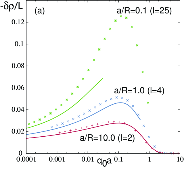
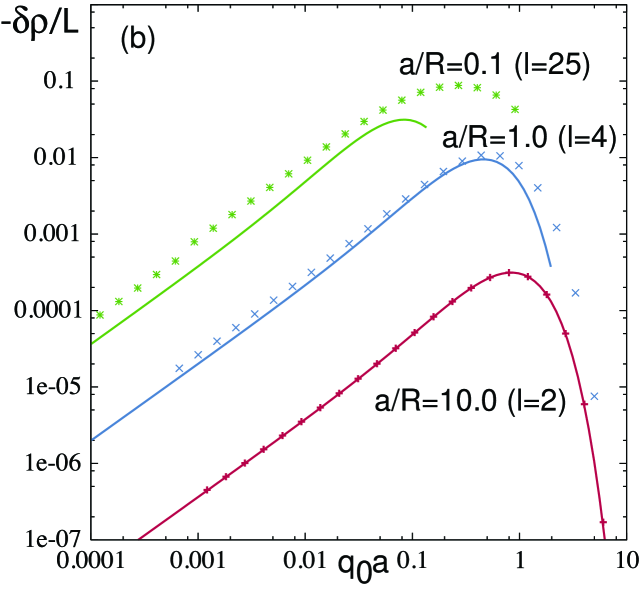
Figure 2: The change in the density of states for (a) Dirichlet and (b) Neumann modes obtained from Eq. (10) at order $l$. The solid curves show the small $R$ expansion of Eq. (11).

Finally, we note that our approach can be extended also to multiple wires and distorted beams. Our results should be relevant to nano-systems composed of 1-dimensional structures and also to other types of fields as, e.g., thermal order parameter fluctuations.

We thank H. Gies for discussions and especially for providing the data of Fig. 1 prior to publication. This work was supported by the DFG through grant EM70/2 (TE), the Istituto Nazionale di Fisica Nulceare (AS), the NSF through grant DMR-04-26677 (MK), and the U. S. Department of Energy (D.O.E.) under cooperative research agreement #DF-FC02-94ER40818 (RLJ & AS).

References

- (1)
- (2) A. N. Cleland and M. L. Roukes, Appl. Phys. Lett. 69, 2653 (1996).
- (3) H. B. Chan, V. A. Aksyuk, R. N. Kleiman, D. J. Bishop, and F. Capasso, Science 291, 1941 (2001).
- (4) V. Sazonova et al., Nature 431, 284 (2004).
- (5) H. B. G. Casimir, Proc. K. Ned. Akad. Wet. 51, 793 (1948).
- (6) M. P. Hertzberg, R. L. Jaffe, M. Kardar and A. Scardicchio, Phys. Rev. Lett. 95, 250402 (2005).
- (7) H. B. G. Casimir and D. Polder, Phys. Rev. 73, 360 (1948).
- (8) M. Brown-Hayes, D. A. R. Dalvit, F. D. Mazzitelli, W. J. Kim, and R. Onofrio, Phys. Rev. A 72, 052102 (2005).
- (9) For a recent study of the co-dimension dependence see A. Scardicchio, Phys. Rev. D 72, 065004 (2005).
- (10) A. Bulgac, P. Magierski, and A. Wirzba, Preprint hep-th/0511056.
- (11) M. Bordag, U. Mohideen, V. M. Mostepanenko, Phys. Rep. 353, 1 (2001).
- (12) M. Schaden and L. Spruch, Phys. Rev. Lett. 84, 459 (2000).
- (13) R. L. Jaffe and A. Scardicchio, Phys. Rev. Lett. 92 070402 (2004); A. Scardicchio and R. L. Jaffe, Nucl. Phys. B 704, 552 (2005) [arXiv:quant-ph/0406041].
- (14) R. Balian and B. Duplantier, Ann. Phys. (New York) 104, 300 (1977); 112, 165 (1978).
- (15) H. Gies, K. Langfeld, and L. Moyaerts, JHEP 0306 018 (2003).
- (16) T. Emig, A. Hanke, R. Golestanian, and M. Kardar, Phys. Rev. Lett. 87, 260402 (2001).
- (17) H. Li and M. Kardar, Phys. Rev. Lett. 67, 3275 (1991); Phys. Rev. A 46, 6490 (1992).
- (18) R. Büscher and T. Emig, Phys. Rev. Lett. 94, 133901 (2005).
- (19) The energies for D and N modes are both half of the EM PFA energy.
- (20) H. Gies, private communication.
- (21) P. W. Milonni, “The Quantum vacuum: An Introduction to quantum electrodynamics,” (Academic Press, New York, 1994).
- (22) A. Scardicchio and R. L. Jaffe, arXiv:quant-ph/0507042.