Universality Class of the Critical Point in the Restricted Primitive Model of Ionic Systems

Abstract

A coarse-grained description of the restricted primitive model is considered in terms of the local charge- and number-density fields. Exact reduction to a one-field theory is derived, and exact expressions for the number-density correlation functions in terms of higher-order correlation functions for the charge-density are given. It is shown that in continuum space the singularity of the charge-density correlation function associated with short-wavelength charge-ordering disappears when charge-density fluctuations are included by following the Brazovskii approach. The related singularity of the individual Feynman diagrams contributing to the number-density correlation functions is cured when all the diagrams are segregated ito disjoint sets according to their topological structure. By performing a resummation of all diagrams belonging to each set a regular expression represented by a secondary diagram is obtained. The secondary diagrams are again segregated into disjoint sets, and the series of all the secondary diagrams belonging to a given set is represented by a hyperdiagram. A one-to-one correspondence between the hyperdiagrams contributing to the number-density vertex functions, and diagrams contributing to the order-parameter vertex functions in a certain model system belonging to the Ising universality class is demonstrated. Corrections to scaling associated with irrelevant operators that are present in the model-system Hamiltonian, and other corrections specific to the RPM are also discussed.

I Introduction

The question of universality class of the critical point associated with a separation into ion-dilute and ion-dense phases in ionic systems has been a subject of an intensive debate for many years. The studies focused mainly on the restricted primitive model (RPM) and we shall focus on the RPM in this work. In the RPM equaly-sized hard spheres with positive and negative charges of the same magnitute are dissolved in a structureless solvent (or in vacuum), and the system is globally charge-neutral. It was predicted theoretically stell:76:0 that the RPM can phase separate, and the separation was observed experimentally and in simulations. Stell put forward arguments that the RPM critical point belongs to the Ising universality class already many years ago hafskjold:82:0 ; stell:92:0 ; stell:95:0 , and the same conclusion followed later from the mesoscopic description described in Refs.ciach:00:0 ; ciach:02:0 ; ciach:05:0 . Earlier simulation results for the RPM in continuum space were not sufficiently accurate to allow for definite conclusions concerning the universality class, however. Moreover, some early experimental results confirmed the Ising criticality japas:90:0 ; narayanan:94:0 , whereas other results were in conformity with the mean-field criticality pitzer:90:0 ; singh:90:0 ; zhang:92:0 or indicated a crossover to the Ising-type critical exponents unusually close to the critical point weingaertner:01:0 ; bianchi:01:0 . In ternary aquaous solutions crossover to multicritical behavior was reported anisimov:00:0 , and a tricritical, rather than a critical point was indeed observed in simulations dickman:99:0 ; panag:99:0 ; diehl:03:0 and predicted theoretically  hoye:97:0 ; stell:99:0 ; dickman:99:0 ; ciach:00:0 ; ciach:01:1 ; kobelev:02:0 ; brognara:02:0 in the RPM with the locations of the ions restricted to the sites of the simple-cubic lattice. The first firm prediction of tricriticaliy for that system appeared in Ref.hoye:97:0 , where a strong argument based on symmetry considerations was given.

The puzzling contradictions described above motivated careful theoretical, simulation and experimental studies of criticality in ionic sytems. In simple words, the Coulombic forces are long-range, and as such might lead to the mean-field (MF) criticality, as noted by Fisher fisher:94:0 . On the other hand, screening effects lead to short-range effective forces, and standard fluid criticality might be expected fisher:94:0 ; stell:95:0 . One of the important issues is the range of the charge-density correlations in the critical region, i.e. beyond the infinite dilution regime fisher:94:0 ; stell:95:0 .

Subsequent precise experiments by Schröer, Wiegand and others wiegand:94:0 ; wiegand:97:0 ; wiegand:98:0 ; wiegand:98:1 ; kleemeier:99:0 ; wagner:02:0 ; wagner:03:0 ; wagner:04:0 showed that by careful identification and elimination of various additional effects (chemical instability, background scattering) Ising criticality is obtaind in all the systems for which MF criticality or tricriticalty, or a delayed crossover were reported previously. The authors of Ref.anisimov:00:0 repeated the experiments and found that the previous observations were associated with long-living metastable states. After the equilibriation time (days) the Ising criticality was observed kostko:04:0 . At present no RPM-like experimental ionic system deviates from the Ising criticality. Recent simulations  orkoulas:99:0 ; yan:99:0 ; luijten:01:0 ; caillol:02:0 ; luijten:02:0 ; kim:03:0 also strongly support the Ising criticality.

On the theoretical side the earlier arguments by Stell stell:92:0 ; stell:95:0 , and the field-theoretic determination of the universality class, briefly sketched in Refs. ciach:00:0 ; ciach:02:0 are still considered as not fully satisfactory. Since exact analytical calculations are impossible, as is also the case for the three-dimensional Ising model, there is a demand for a theory analogous to the renormalization-group (RG) theory in simple fluids amit:84:0 ; zinn-justin:89:0 . The latter is restricted to short-range interactions, and is not directly applicable to the Coulombic forces.

In this work the theory introduced in Ref.ciach:00:0 is further developed, and exact derivations as well as technical details are explained on a formal basis. We start with the mesoscopic description first proposed in Ref.ciach:00:0 and described in more detail in Refs.ciach:05:0 ; ciach:05:2 . In the coarse-grained description local distributions of the ionic species occur with a probability proportional to the Boltzmann factor $\exp(-\beta\Omega^{MF}[\phi({\bf x})\rho({\bf x})])$. Here $\Omega^{MF}[\phi({\bf x})\rho({\bf x})]$ is the grand potential in the system with the charge- and number densities constrained to be $\phi({\bf x})$ and $\rho({\bf x})$ in an infinitesimal (’mesoscopic’) volume $d{\bf x}$ centered at the space position ${\bf x}$. It seems natural to reduce the two-field theory to a one-field theory depending only on the number-density of ions, which should be a proper order parameter for the gas-liquid type transition. However, in the RPM only charges interact, and it is not possible to perform such a reduction in a simple way. On the other hand, because there are no interactions between the masses in the RPM, the field $\rho({\bf x})$ can be integrated out easily. In sec.3 we reduce the two-field theory to the one-field theory of the field $\phi({\bf x})$, with the Boltzmann factor $\propto\exp(-\beta{\cal H}_{eff}[\phi])$. The particular feature of the one-field theory is that the second functional derivative of ${\cal H}_{eff}[\phi]$ assumes a minimum for the wavenumber $k_{b}\neq 0$ in Fourier representation, and the higher-order terms $\propto\int_{\bf x}{\cal A}_{2n}\phi^{2n}({\bf x})$ have the property that for low valuse of the average number density ${\cal A}_{4}<0$ and ${\cal A}_{2n}>0$ for $n>2$. We find exact expressions for the number-density correlation functions in terms of the higher-order correlation functions for $\phi({\bf x})$ in the one-field theory.

In order to determine the scaling properties of the connected number-density correlation functions we consider the corresponding Feynman diagrams in the (formal) perturbation expansion in ${\cal A}_{2n}$. In sec.4 we study the two-point charge-density correlation function $G_{\phi\phi}$. In the Gaussian approximation $\tilde{G}^{0}_{\phi\phi}(k)$ is singular for the wavenumber $k_{b}\neq 0$. The singularity is removed beyond the Gaussian approximation by following the Brazovskii theory brazovskii:75:0 . We segregate all Feynman diagrams for any given connected number-density correlation function into disjoint sets according to a prescription described in sec.5. By summing all diagrams in each set we obtain a finite expression, which can be represented by a skeleton diagram with lines representing the charge-density correlation function. We call such a series of diagrams ’a secondary diagram’. In this way we cure the artificial singularity of individual diagrams following from the singularity of $\tilde{G}^{0}_{\phi\phi}(k_{b})$.

The secondary diagrams are again segregated into disjoint sets, according to their topological properties, as explained in sec. 5. A series of the secondary diagrams belonging to a particular set can be represented by a hyperdiagram. The hyperdiagrams are associated with the same expressions for $k\to 0$ as the corresponding diagrams in a model system with the Hamiltonian belonging to the Ising universality class, which contains also irrelevant operators. We could repeat the whole procedure of regularization of the hyperdiagrams, renormalization of the coupling constants and solve the flow equations describing the evolution of the renormalized coupling constants under changing the length scale, but this has already been done amit:84:0 ; zinn-justin:89:0 for the model Hamiltonian yielding the same expressions for the vertex functions in the (formal) perturbation expansion. In sec.5 we also describe corrections to scaling specific for the RPM. The last section contains a short summary.

II Background

II.1 Coarse-grained description for the RPM.

In the field-theoretic, coarse-grained approach we consider local densities of the ionic species in mesoscopic regions $d{\bf x}$ around each point ${\bf x}$, $\rho_{\alpha}({\bf x})$, where $\alpha=+,-$. For fixed temperature and chemical potential the probability density that the local densities assume a particular form $\rho_{+}({\bf x})$, $\rho_{-}({\bf r})$ is given by ciach:05:0 ; ciach:05:2

$$p[\rho_{+}^{*}({\bf x}),\rho_{-}^{*}({\bf x})]=\Xi^{-1}\exp(-\beta\Omega^{MF}[\rho_{+}^{*},\rho_{-}^{*}]),$$ (1)

where

$$\Xi=\int D\rho^{*}_{+}\int D\rho^{*}_{-}\exp(-\beta\Omega^{MF}[\rho_{+}^{*},\rho_{-}^{*}]),$$ (2)

$\beta=1/kT$ with $k$ the Boltzmann constant and $T$ temperature, and we introduced dimensionless densities

$$\rho^{*}_{\alpha}=\rho_{\alpha}\sigma_{+-}^{3},$$ (3)

where $\sigma_{+-}=(\sigma_{+}+\sigma_{-})/2$ is the sum of radii. In the above $\Omega^{MF}[\rho_{+}^{*},\rho_{-}^{*}]$ is the grand potential in the system where the local concentrations of the two ionic species are constrained to be $\rho^{*}_{+}({\bf r})$, $\rho^{*}_{-}({\bf x})$,

$$\Omega^{MF}[\rho^{*}_{+},\rho^{*}_{-}]=F_{h}[\rho^{*}_{+},\rho^{*}_{-}]+U^{PM}[\rho^{*}_{+},\rho^{*}_{-}]-\mu_{\alpha}\int_{\bf x}\rho^{*}_{\alpha}({\bf x}),$$ (4)

We use simplified notation $\int_{\bf x}\equiv\int d{\bf x}$ throghout the whole paper. In Eq.(4) $F_{h}$ is the Helmholtz free energy of the hard-core reference system, and we shall limit ourselves to the local-density approximation $F_{h}[\rho^{*}_{+},\rho^{*}_{-}]=\int d{\bf x}f_{h}(\rho^{*}_{+}({\bf x}),\rho^{*}_{-}({\bf x}))$. In principle, more accurate approximations for $F_{h}[\rho^{*}_{+},\rho^{*}_{-}]$ could be adopted. In the local density approximation

$$\beta\frac{\partial^{2}f_{h}}{\partial\rho_{\alpha}^{*}\partial\rho_{\beta}^{*}}=\frac{\delta^{Kr}_{\alpha,\beta}}{\rho^{*}_{\alpha}}-c_{h}(\rho^{*}),$$ (5)

where the first term results from the ideal entropy of mixing,

$$\rho^{*}=\rho^{*}_{+}+\rho^{*}_{-},$$ (6)

and $c_{h}(\rho^{*})$ is the volume integral over the hard-sphere contribution to the Ornstein-Zernike direct correlation function.

In this work we focus on the RPM. In the RPM $\delta^{2}\Omega^{MF}/\delta\rho^{*}_{\alpha}\delta\rho^{*}_{\beta}$ can be easily diagonalized due to the symmetry of the interaction potentials, and the eigenmodes have a natural physical interpretation. The first eigenmode is the number-density deviation of ionic species from the most probable value,

$$\eta({\bf x})=\rho^{*}({\bf x})-\rho^{*}_{0},$$ (7)

and the second mode is the local charge-density in $e$-units ($e=e_{+}=|e_{-}|$),

$$\phi({\bf x})=\rho^{*}_{+}({\bf x})-\rho^{*}_{-}({\bf x}).$$ (8)

The electrostatic energy is

$$\beta U^{RPM}[\phi]=\frac{\beta^{*}}{2}\int_{{\bf x}_{1}}\int_{{\bf x}_{2}}\phi({\bf x}_{1})V({\bf x}_{1}-{\bf x}_{2})\phi({\bf x}_{2}),$$ (9)

$$\beta^{*}=\frac{1}{T^{*}}=\frac{\beta e^{2}}{D\sigma},$$ (10)

$$V({\bf x})=\frac{\theta(x-\sigma_{\alpha\beta})}{x},$$ (11)

and $x=|{\bf x}|$. In the following, distances will be measured in $\sigma_{+-}=\sigma$ units. In Eq. (9) the contributions to the electrostatic energy coming from overlapping hard spheres are excluded because of the form of the potential $V$ (see Eq.(11)).

In the field theory introduced above the physical quantities are obtained by averaging over all fields $\rho_{+}^{*}$, $\rho_{-}^{*}$ (or over $\phi$ and $\eta$ in the RPM) with the Boltzmann factor (1), and the grand potential $\Omega$ is

$$-\beta\Omega=\log\Xi.$$ (12)

For small amplitudes of the fields $\phi$ and $\eta$ the functional (4) can be expanded about its value $\Omega^{MF}_{0}$ at the minimum,

$$\Delta\Omega^{MF}=\Omega^{MF}-\Omega^{MF}_{0}=\Omega_{2}+\Omega_{int}.$$ (13)

Here $\Omega_{2}$ denotes the Gaussian part of the functional. In terms of the eigenmodes the Gaussian part of the functional (13) assumes the form

$$\beta\Omega_{2}={1\over 2}\int_{\bf k}\Bigg{[}\tilde{C}_{\phi\phi}^{0}({\bf k})\tilde{\phi}({\bf k})\tilde{\phi}(-{\bf k})+\tilde{C}_{\eta\eta}^{0}({\bf k})\tilde{\eta}({\bf k})\tilde{\eta}(-{\bf k})\Bigg{]},$$ (14)

where we simplify the notation for the integrals in the Fourier space $\int_{\bf k}\equiv\int{d{\bf k}\over(2\pi)^{3}}$. By using (5) we obtain

$$\tilde{C}_{\phi\phi}^{0}({\bf k})=\rho_{0}^{*-1}+\beta^{*}\tilde{V}({\bf k}),$$ (15)

and

$$\tilde{C}_{\eta\eta}^{0}({\bf k})=\gamma_{0,2}=\beta{\partial^{2}f_{h}\over\partial\rho^{*2}}|_{\phi=0,\rho^{*}=\rho^{*}_{0}}.$$ (16)

In the continuum-space RPM the Fourier transform of the potential (11) has the form

$$\tilde{V}(k)=\frac{4\pi\cos k}{k^{2}},$$ (17)

where $k=|{\bf k}|$ is in $\sigma^{-1}$ units. The wavenumber corresponding to the minimum of the potential $\tilde{V}(k)$ is $k_{b}\neq 0$ ciach:00:0 . The explicit form of $\gamma_{0,2}$ depends on the approximation for the hard-sphere reference-system; in any case, in the absence of short-range attractive forces it is a positive function of $\rho^{*}_{0}$. Hence, $\eta$ is a noncritical field. On the other hand, $\tilde{C}_{\phi\phi}^{0}(k)$ can vanish for $k\neq 0$. The boundary of stability of $\Delta\Omega^{MF}$ in the $(\rho^{*},T^{*})$ phase space is given by

$$\tilde{C}_{\phi\phi}^{0}(k_{b})=0.$$ (18)

The critical fluctuations are thus $\tilde{\phi}({\bf k}_{b})$.

The $\Omega_{int}$ has the expansion

$$\beta\Omega_{int}[\phi,\eta]=\sum_{m,n}^{\prime}\int_{{\bf x}}\frac{\gamma_{2m,n}}{(2m)!n!}\phi({\bf x})^{2m}\eta({\bf x})^{n}.$$ (19)

where $\sum_{m,n}^{{}^{\prime}}$ denotes the summation with $2m+n\geq 3$, and $\gamma_{2m,n}$ denotes the appropriate derivative of $f_{h}$ at $\phi=0$ and $\eta=0$.

II.2 Ising Universality Class and Scaling

The universality class of a given system is associated with a particular scaling form of the singular part of the thermodynamic potential in the critical region, or, equivalently, by the scaling properties of the large-distance part of the connected correlation functions. In particular, the Ising universality class is represented by the standard $\varphi^{4}$ theory with the Hamiltonian

$${\cal H}^{I}[\varphi]=\frac{1}{2}\int_{\bf k}(t_{0}+k^{2})\tilde{\varphi}({\bf k})\tilde{\varphi}(-{\bf k})+\int_{\bf x}\Big{(}-H_{0}\varphi({\bf x})+\frac{u_{0}}{4!}\varphi^{4}({\bf x})\Big{)}.$$ (20)

The (renormalized) connected $N$-point correlation function for the field $\varphi$ scales in the real-space representation according to amit:84:0

$$G^{R}_{N}({\bf x}_{1},...,{\bf x}_{N};t,u,H)=t^{N\beta}G^{R}_{N}({\bf x}_{1}t^{\nu},...,{\bf x}_{N}t^{\nu};1,u^{*},Ht^{-\Delta}),$$ (21)

where $t$, $H$ and $u$ are the renormalized coupling constants corresponding to the bare couplings $t_{0}$, $H_{0}$ and $u_{0}$ respectively, and $u^{*}$ is the fixed point of the RG flow of $\bar{u}(\ell)$ upon rescaling the length unit, $x\to x\ell$ for $\ell\to 0$, where $\bar{u}(\ell=1)=u$ amit:84:0 . In the case of a magnet $t$ and $H$ correspond to reduced temperature and magnetic field respectively. The two independent critical exponents $\beta$ and $\Delta$ are related to the other exponents via scaling relations amit:84:0 . In particular, $\beta=\nu(d-2+\eta)/2$ and $\Delta=\nu(d+2-\eta)/2$.

Our purpose here is to determine the universality class of the RPM critical point. Thus, we have to study scaling properties of the correlation functions for the number-density field $\eta({\bf x})$ near the critical point of the phase separation, i.e. in the phase space region where $\langle\phi\rangle=0$. It is the correlation function for large separations, which may lead to divergent susceptibility and obeys scaling. In determining the universality class of a critical point one can separate the correlation function into a long- and a short-distance parts, and neglect the latter. In the next section we construct an effective one-field theory which allows for a determination of nonlocal parts of the number-density correlation functions.

III Effective field theory

In this section we derive an exact effective Hamiltonian ${\cal H}_{eff}[\phi]$, such that the grand potential is given by $\Omega=-kT\log\int D\phi\exp(-\beta{\cal H}_{eff}[\phi])$. Next we derive exact expressions for the nonlocal parts of the number-density correlation functions in terms of higher-order correlations for the field $\phi$, with the Boltzmann factor $\exp(-\beta{\cal H}_{eff}[\phi])$. We also introduce generating functionals for the relevant correlation and vertex functions.

III.1 Derivation of the effective functional

The functional $\Delta\Omega^{MF}[\phi,\eta]$ (Eqs.(13) and (4)) can be split into two parts,

$$\Delta\Omega^{MF}[\phi,\eta]=\Omega_{\phi}[\phi]+\Omega_{\eta}[\phi,\eta]$$ (22)

where

$$\beta\Omega_{\phi}[\phi]=\frac{1}{2}\langle\phi|C^{0}_{\phi\phi}|\phi\rangle+\sum_{m=2}\frac{\gamma_{2m,0}}{(2m)!}\langle 1|\phi^{2m}\rangle,$$ (23)

$$\beta\Omega_{\eta}[\phi,\eta]=\frac{1}{2}\langle\eta|C^{0}_{\eta\eta}|\eta\rangle+\sum_{m,n}^{\prime\prime}\frac{\gamma_{2m,n}}{(2m)!n!}\langle\phi^{2m}|\eta^{n}\rangle,$$ (24)

and where $\sum_{m,n}^{\prime\prime}$ indicates a summation with $n\geq 1$ and $2m+n\geq 3$. In the real space representation $\phi$ and $\eta$ are real functions. For convenience we use the Dirac brac-kets notation for the scalar product

$$\langle f|g\rangle\equiv\int_{\bf x}f^{*}({\bf x})g({\bf x})=\int_{\bf k}\tilde{f}({\bf k})\tilde{g}(-{\bf k}),$$ (25)

and $|A|f\rangle$ denotes the operator $A$ acting on the state $|f\rangle$. In particular, when in real-space representation $A$ has a functional form $A({\bf x},{\bf x}^{\prime})$, then

$$|A|f\rangle\equiv\int_{{\bf x}^{\prime}}A({\bf x},{\bf x}^{\prime})f({\bf x}^{\prime}).$$ (26)

We introduce a functional of two external fields $J({\bf x})$ and $v({\bf x})$ by

$$\Delta\Xi[J,v]=\int D\phi e^{\langle J|\phi\rangle}e^{-\beta\Omega_{\phi}[\phi]}\Xi_{\eta}[\phi,v]$$ (27)

where

$$\Xi_{\eta}[\phi,v]=\int D\eta e^{\langle v|\eta\rangle}e^{-\beta\Omega_{\eta}[\phi,\eta]}.$$ (28)

Because in the pure RPM (no other interactions included) $C_{\eta\eta}^{0}({\bf x}_{1},{\bf x}_{2})=C_{\eta\eta}^{0}\delta({\bf x}_{1},{\bf x}_{2})$ (see Eq.(16)), Eq.(24) can be rewriten in the form

$$\beta\Omega_{\eta}[\phi,\eta]=\int_{\bf x}\beta\omega_{\eta}(\phi({\bf x}),\eta({\bf x})),$$ (29)

and we immediately obtain the exact result

$$\log\Xi_{\eta}[\phi,v]=\int_{\bf x}\omega(\phi({\bf x}),v({\bf x})),$$ (30)

where

$$\omega(\phi({\bf x}),v({\bf x}))=\log\Bigg{[}\int d(\eta({\bf x}))e^{-\beta\omega_{\eta}(\phi({\bf x}),\eta({\bf x}))}e^{v({\bf x})\eta({\bf x})}\Bigg{]}.$$ (31)

The integrand $\omega(\phi({\bf x}),0)$ in Eq. (30) can be expanded in a Taylor series with respect to $\phi({\bf x})$ and we obtain the formal expression

$$\omega(\phi({\bf x}),0)=\sum_{m=0}^{\infty}\frac{f_{2m}(\rho_{0}^{*})}{(2m)!}\phi^{2m}({\bf x}),$$ (32)

where the explicit forms of $f_{2m}(\rho_{0}^{*})$ depend on the form of the Helmholtz free-energy density of the hard-sphere reference system. By substituting the above form of $\Xi_{\eta}$ into Eq.(27) we obtain

$$\Delta\Xi[J,0]=Z_{\eta}\Xi_{0}[J],\hskip 28.45274pt\Xi_{0}[J]=\int D\phi e^{\langle J|\phi\rangle}e^{-\beta{\cal H}_{eff}[\phi]}$$ (33)

where $\log Z_{\eta}=\int_{\bf x}f_{0}(\rho_{0}^{*})$ ($\log\Delta\Xi[J,0]$ is an extensive quantity),

$$\beta{\cal H}_{eff}[\phi]=\frac{1}{2}\langle\phi|{\cal C}_{\phi\phi}^{0}|\phi\rangle+\sum_{m=2}^{\infty}\frac{{\cal A}_{2m}}{(2m)!}\int_{\bf x}\phi^{2m}({\bf x}),$$ (34)

$${\cal C}_{\phi\phi}^{0}({\bf x},{\bf x}^{\prime})=C_{\phi\phi}^{0}({\bf x},{\bf x}^{\prime})+f_{2}(\rho_{0}^{*})\delta({\bf x}-{\bf x}^{\prime})$$ (35)

and

$${\cal A}_{2m}=\gamma_{2m,0}+f_{2m}(\rho_{0}^{*}).$$ (36)

Eqs.(33)-(36) define the effective functional.

Eq.(28) can be written in a more general form, valid also beyond the RPM (i.e. for nonlocal $C^{0}_{\eta\eta}$), zinn-justin:89:0 ; amit:84:0

$$\Xi_{\eta}[\phi,v]=Z_{\eta}^{0}\cdot\exp\Bigg{[}-\sum_{m,n}^{\prime\prime}\frac{\gamma_{2m,n}}{(2m)!n!}\int_{\bf x}\phi^{2m}({\bf x})\frac{\delta^{n}}{\delta v({\bf x})^{n}}\Bigg{]}e^{\frac{1}{2}\langle v|G_{\eta\eta}^{0}|v\rangle}.$$ (37)

In the above the constant is $Z^{0}_{\eta}=\int Dfe^{-\frac{1}{2}\langle f|C_{\eta\eta}^{0}|f\rangle}$, and

$$Z_{\eta}=Z_{\eta}^{0}\exp\Bigg{[}-\sum_{n=3}^{\infty}\frac{\gamma_{0,n}}{n!}\int_{\bf x}\frac{\delta^{n}}{\delta v({\bf x})^{n}}\Bigg{]}e^{\frac{1}{2}\langle v|G^{0}_{\eta\eta}|v\rangle}|_{v=0}.$$ (38)

Nonvanishing contributions to $\Xi_{\eta}[\phi,0]$ result from an even number of differentiations in Eq.(37) with respect to $v$. In the case of the RPM $\langle f|G_{\eta\eta}^{0}|f\rangle=G_{\eta\eta}^{0}\langle f|f\rangle$, and a double differentiation with respect to $v$ gives a factor $G_{\eta\eta}^{0}=1/C_{\eta\eta}^{0}$. The Wick theorem allows to represent $\Xi_{\eta}[\phi,0]$ as a sum of all vacuum Feynman diagrams (no external points) with vertices $\gamma_{2m,n}\phi^{2m}({\bf x})$ such that $n\geq 1$ and $2m+n\geq 3$, all at the same point ${\bf x}$. From the vertex $\gamma_{2m,n}\phi^{2m}({\bf x})$ there emanate $n$ $\eta$-lines, and all $\eta$-lines have to be paired. Lines connecting different vertices as well as loops represent $G_{\eta\eta}^{0}$. Finally, each diagram is integrated over ${\bf x}$.

$\log\Xi_{\eta}[\phi,0]=\int_{\bf x}\omega(\phi({\bf x}),0)$ is represented by all connected vacuum diagrams described above amit:84:0 ; zinn-justin:89:0 . $\omega(\phi({\bf x}),0)$ is represented by the same diagrams, except that there is no integration over ${\bf x}$. The term proportional to $\phi^{2m}({\bf x})$ in the expansion of $\omega(\phi({\bf x}),0)$ in Eq.(32) is represented by the sum of all connected diagrams, such that each diagram in the sum contains a certain number $N$ of vertices $\gamma_{2m_{j},n_{j}}\phi^{2m_{j}}({\bf x})$, and $\sum_{j=1}^{N}m_{j}=m$. In particular, $f_{2}\phi^{2}({\bf x})$ is represented by a sum of all connected vacuum diagrams, where each diagram in the sum contains an arbitrary number of vertices $\gamma_{0,n}$, and a single vertex $\gamma_{2,k}\phi^{2}({\bf x})$, where $k$ is arbitrary. There are no zero-loop contributions to $f_{2}\phi^{2}({\bf x})$, and the one-loop contributions are shown in Fig.1.

Figure 1: One-loop diagrams contributing to $f_{2}\phi^{2}({\bf x})$. Thick lines and loops represent $G^{0}_{\eta\eta}$ and thin lines represent $\phi$. Vertices with $2m$ thin lines and $n$ thick lines represent $\gamma_{2m,n}$.

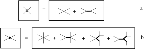
Figure 2: Zero-loop diagrams contributing to ${\cal A}_{4}\phi^{4}({\bf x})$ (a) and ${\cal A}_{6}\phi^{6}({\bf x})$ (b). Thick lines represent $G^{0}_{\eta\eta}$ and thin lines represent $\phi$. Vertices with $2m$ thin lines and $n$ thick lines represent $\gamma_{2m,n}$.

Figure 3: One-loop diagrams contributing to ${\cal A}_{4}\phi^{4}({\bf x})$. Thick lines and loops represent $G^{0}_{\eta\eta}$ and thin lines represent $\phi$. Vertices with $2m$ thin lines and $n$ thick lines represent $\gamma_{2m,n}$.

The zero-loop diagrams contributing to ${\cal A}_{4}\phi^{4}({\bf x})$ and ${\cal A}_{6}\phi^{6}({\bf x})$ are shown in Fig.2, and one loop diagrams contributing to ${\cal A}_{4}\phi^{4}({\bf x})$ are shown in Fig.3. In these diagrams each thin line emanating from the vertex at ${\bf x}$ represents $\phi({\bf x})$, thick lines represent $G_{\eta\eta}^{0}$, and the diagrams are multiplied by appropriate symmetry factors amit:84:0 ; zinn-justin:89:0 . ${\cal A}_{2m}$ is represented by a sum of the corresponding diagrams with amputated $\phi({\bf x})$-lines.

The above perturbation approach is convenient for a development of approximate theories. Let us compare the above exact theory with the weighted-field (WF) approximation developed in Refs.ciach:00:0 ; ciach:04:1 . The WF approximation is of the mean-field type with respect to the field $\eta$, because the effective functional is obtained by minimizing $\Delta\Omega^{MF}$ with respect to $\eta$ for a given field $\phi$. ${\cal H}_{eff}[\phi]$ given in Eq.(34) has the same functional form as in the WF theory. Moreover, in the zero-loop approximation the term $f_{2}$ vanishes, and the coefficients ${\cal A}_{2m}$ reduce to those obtained previously in Ref. ciach:04:1 . Thus, in the zero-loop approximation the above exact effective theory reduces to the WF approximation, as expected.

In the effective theory derived above we can rewrite $\Xi_{0}[J]$ in the form

$$\Xi_{0}[J]=Z_{\phi}\Xi_{1}[J],\hskip 28.45274pt\Xi_{1}[J]=e^{-\sum_{m=2}\frac{{\cal A}_{2m}}{2m!}\int_{\bf x}\frac{\delta^{2m}}{\delta J({\bf x})^{2m}}}e^{\frac{1}{2}\langle J|G_{\phi\phi}^{0}|J\rangle},$$ (39)

where $Z_{\phi}=\int Dfe^{-\frac{1}{2}\langle f|{\cal C}_{\phi\phi}^{0}|f\rangle}$, and the charge-density correlation function in the Gaussian approximation, $G_{\phi\phi}^{0}$, is inverse to ${\cal C}_{\phi\phi}^{0}$,

$$\tilde{G}_{\phi\phi}^{0}(k)=1/\tilde{\cal C}_{\phi\phi}^{0}(k).$$ (40)

By applying the Wick theorem we can represent $\Xi_{1}[0]$ by vacuum diagrams with ’hypervertices’ ${\cal A}_{2m}$ from which there emanate $2m$ $\phi$-lines. All lines are paired, and the line connecting vertices at ${\bf x}_{1}$ and ${\bf x}_{2}$ represents $G_{\phi\phi}^{0}({\bf x}_{1},{\bf x}_{2})$. The name ’hypervertex’ used in Ref.ciach:04:1 comes from the form of ${\cal A}_{2m}$ in the original, two-field theory (see Eq.(36) and Fig.2), but in the effective one-field theory ${\cal A}_{2m}$ are just usual vertices. For simplicity, in the rest of this paper we shall use the name ’vertex’ for ${\cal A}_{2m}$.

III.2 Stability of the functional ${\cal H}_{eff}$

The effective functional of the form (34) was already studied in the WF theory ciach:04:1 ; ciach:05:0 , which is equivalent to the zero-loop approximation for $f_{2}$ and ${\cal A}_{2n}$. Beyond the WF approximation the Gaussian correlation function $\tilde{G}_{\phi\phi}^{0}({\bf k})$ diverges for the same wavevector ${\bf k}={\bf k}_{b}\neq{\bf 0}$ as found in Ref.ciach:00:0 , but along the spinodal line

$$T^{*}_{b}=-\rho_{0}^{*}\frac{\tilde{V}({\bf k}_{b})}{1+\rho_{0}^{*}f_{2}(\rho_{0}^{*})},$$ (41)

which is shifted compared to that found in the WF theory, where $f_{2}=0$ (note that $\tilde{V}({\bf k}_{b})<0$). We assume that the denominator is positive for the relevant range of $\rho_{0}^{*}$. For particular forms of $f_{h}$ this assumption remains to be verified. Divergent $\tilde{G}_{\phi\phi}^{0}({\bf k}_{b})$ for ${\bf k}_{b}\neq{\bf 0}$ indicates that our theory belongs to the class of the Brazovskii field theories brazovskii:75:0 .

Another important property of our WF theory is the fact that for low densities, $\rho_{0}^{*}<\rho_{tc}^{*}$, the vertex ${\cal A}_{4}$ becomes negative, and ${\cal A}_{2n}>0$ for $n>2$ ciach:00:0 ; ciach:04:1 . This property leads to a tricritical point on the sc lattice ciach:03:0 ; ciach:04:1 , and to a gas-liquid type instability in continuum and some other lattice systems ciach:03:0 ; ciach:04:0 , in agreement with simulation results panag:99:0 ; diehl:03:0 ; diehl:05:0 . Based on the WF and the simulation results we focus here on the general field theory having the property that ${\cal A}_{4}(\rho_{0}^{*})$ becomes negative for sufficiently low densities, with ${\cal A}_{6}>0$ ciach:05:0 ; ciach:04:1 . Within the exact theory developed above this assumption remains to be verified for particular forms of the reference system. Negative values of ${\cal A}_{4}$ for low densities bring our field theory in the corresponding part of the phase diagram beyond the class of the Brazovskii-type field theories, where ${\cal A}_{4}>0$.

III.3 Correlation functions in the effective field theory

The correlation functions for the field $\phi$ can be obtained in a standard way from their generating functional $\Delta\Xi[J,v]$ given in Eq.(27),

$$\langle\langle\phi^{k_{1}}({\bf x}_{1})...\phi^{k_{n}}({\bf x}_{n})\rangle\rangle=\frac{1}{\Delta\Xi}\frac{\delta^{k_{1}+...+k_{n}}\Delta\Xi}{\delta J({\bf x}_{1})^{k_{1}}...\delta J({\bf x}_{n})^{k_{n}}}|_{J=0,v=0},$$ (42)

and the connected correlation functions are given by amit:84:0 ; zinn-justin:89:0

$$\langle\langle\phi^{k_{1}}({\bf x}_{1})...\phi^{k_{n}}({\bf x}_{n})\rangle\rangle^{con}=\frac{\delta^{k_{1}+...+k_{n}}\log\Delta\Xi}{\delta J({\bf x}_{1})^{k_{1}}...\delta J({\bf x}_{n})^{k_{n}}}|_{J=0,v=0}.$$ (43)

$\langle\langle...\rangle\rangle$ denotes the average in the original two-field theory. From (27) and (33) we obtain

$$\langle\langle\phi^{k_{1}}({\bf x}_{1})...\phi^{k_{n}}({\bf x}_{n})\rangle\rangle=\langle\phi^{k_{1}}({\bf x}_{1})...\phi^{k_{n}}({\bf x}_{n})\rangle,$$ (44)

where $\langle...\rangle$ denotes averaging in the effective one-field theory. The connected correlation function $\langle\phi^{k_{1}}({\bf x}_{1})...\phi^{k_{n}}({\bf x}_{n})\rangle^{con}$ is represented by a sum of all connected diagrams containing external points ${\bf x}_{1},...{\bf x}_{n}$ from which there emanate $k_{1},...,k_{n}$ $\phi$-lines respectively, and vertices ${\cal A}_{2m}$ from which there emanate $2m$ $\phi$-lines. All lines are paired. A line connecting a vertex or an external point at ${\bf x}_{1}$ with a vertex or an external point at ${\bf x}_{2}$ represents $G_{\phi\phi}^{0}({\bf x}_{1},{\bf x}_{2})$ amit:84:0 ; zinn-justin:89:0 .

Let us consider the number-density correlation functions defined by

$$\langle\langle\eta({\bf x}_{1})...\eta({\bf x}_{n})\rangle\rangle=\frac{1}{\Delta\Xi}\frac{\delta^{n}\Delta\Xi}{\delta v({\bf x}_{1})...\delta v({\bf x}_{n})}|_{J=0,v=0}.$$ (45)

From (27) we have

$$\langle\langle\eta({\bf x}_{1})...\eta({\bf x}_{n})\rangle\rangle=\frac{1}{\Delta\Xi}\int D\phi e^{-\beta\Omega_{\phi}[\phi]}D_{n}[{\bf x}_{1},...,{\bf x}_{n}|\phi]$$ (46)

where

$$D_{n}[{\bf x}_{1},...,{\bf x}_{n}|\phi]=\frac{\delta^{n}\Xi_{\eta}[\phi,v]}{\delta v({\bf x}_{1})...\delta v({\bf x}_{n})}|_{v=0}.$$ (47)

By using Eq.(37) for local $C_{\eta\eta}^{0}$, in the case of ${\bf x}_{1}\neq{\bf x}_{2}\neq...\neq{\bf x}_{n}$ we obtain

$$D_{n}[{\bf x}_{1},...,{\bf x}_{n}|\phi]=Z^{0}_{\eta}\cdot G_{\eta\eta}^{0n}\exp\Bigg{[}-\sum_{m,n}^{{}^{\prime\prime}}\int_{\bf x}\frac{\gamma_{2m,n}}{(2m)!n!}\phi^{2m}({\bf x})\frac{\delta^{n}}{\delta v({\bf x})^{n}}\Bigg{]}v({\bf x}_{1})...v({\bf x}_{n})e^{\frac{1}{2}G_{\eta\eta}^{0}\langle v|v\rangle}|_{v=0}.$$ (48)

When ${\bf x}_{i}={\bf x}_{j}$ for at least one pair of external points, there are additional contributions to $D_{n}[{\bf x}_{1},...,{\bf x}_{n}|\phi]$ amit:84:0 ; zinn-justin:89:0 . We shall focus only on the case of ${\bf x}_{1}\neq{\bf x}_{2}\neq...\neq{\bf x}_{n}$. From the Wick theorem it follows that in the case of the RPM each diagram contributing to $D_{n}$ consists of $n$ disjoint diagrams, each of them containing a single external point, and of vacuum diagrams. Thus,

$$D_{n}[{\bf x}_{1},...,{\bf x}_{n}|\phi]=\Xi_{\eta}[\phi,0]\prod_{i=1}^{n}\zeta({\bf x}_{i}),$$ (49)

where

$$\zeta({\bf x}_{i})=\sum_{m=0}\frac{a_{m}}{m!}\phi^{2m}({\bf x}_{i}),$$ (50)

and $a_{m}$ are functions of $\rho_{0}^{*}$ depending on the form of the free energy in the hard-sphere reference system. Each term $a_{m}\phi^{2m}({\bf x}_{i})$ in Eq.(50) is represented by the sum of all connected diagrams containing a single external point ${\bf x}_{i}$, and an arbitrary number $N$ of vertices $\gamma_{2m_{j},n_{j}}\phi^{2m_{j}}({\bf x}_{i})$ that satisfy $\sum_{j=1}^{N}m_{j}=m$. Eqs. (49) and (50) are of course immediately obtained by a direct differentiation of the exact formula (30).

By substituting Eq.(49) into Eq.(45) we obtain for ${\bf x}_{1}\neq{\bf x}_{2}\neq...\neq{\bf x}_{n}$

$$\langle\langle\eta({\bf x}_{1})...\eta({\bf x}_{n})\rangle\rangle=\frac{1}{\Xi_{0}}\int D\phi e^{-\beta{\cal H}_{eff}[\phi]}\zeta({\bf x}_{1})...\zeta({\bf x}_{n})=\langle\zeta({\bf x}_{1})...\zeta({\bf x}_{n})\rangle.$$ (51)

The connected correlation function for the number-density fields can be written in the form

$$\langle\langle\eta({\bf x}_{1})...\eta({\bf x}_{n})\rangle\rangle^{con}=\langle\zeta({\bf x}_{1})...\zeta({\bf x}_{n})\rangle^{con}=\sum_{m_{1}=1}^{\infty}\frac{a_{m_{1}}}{m_{1}!}...\sum_{m_{n}=1}^{\infty}\frac{a_{m_{n}}}{m_{n}!}\langle\phi^{2m_{1}}({\bf x}_{1})...\phi^{2m_{n}}({\bf x}_{n})\rangle^{con}.$$ (52)

The above equation shows that for ${\bf x}_{1}\neq{\bf x}_{2}\neq...\neq{\bf x}_{n}$ the connected number-density correlation functions are given in terms of higher-order charge-density correlation functions with the Boltzmann factor $\propto\exp\big{(}-\beta{\cal H}_{eff}[\phi]\big{)}$. We introduce for convenience an additional field

$$\psi({\bf x})=a_{1}\phi^{2}({\bf x}),$$ (53)

where

$$a_{1}=G^{0}_{\eta\eta}\Big{(}-\frac{\gamma_{2,1}}{2}+...\Big{)},$$ (54)

and we rewrite Eq.(52) as follows

$$\langle\zeta({\bf x}_{1})...\zeta({\bf x}_{n})\rangle^{con}=\sum_{m_{1}=1}^{\infty}\frac{a_{m_{1}}}{a_{1}^{m_{1}}m_{1}!}...\sum_{m_{n}=1}^{\infty}\frac{a_{m_{n}}}{a_{1}^{m_{n}}m_{n}!}\langle\psi^{m_{1}}({\bf x}_{1})...\psi^{m_{n}}({\bf x}_{n})\rangle^{con}=$$ (55)

$$\langle\psi({\bf x}_{1})...\psi({\bf x}_{n})\rangle^{con}+\frac{a_{2}}{a_{1}^{2}}\langle\psi^{2}({\bf x}_{1})...\psi({\bf x}_{n})\rangle^{con}+....$$

Note that $\langle\zeta({\bf x}_{1})...\zeta({\bf x}_{n})\rangle^{con}$ is given in terms of $\langle\psi({\bf x}_{1})...\psi({\bf x}_{m})\rangle^{con}$ with $m\geq n$, such that for $m>n$ some of the external points are identical, and the number of distinct external points is $n$. $\langle\psi({\bf x}_{1})...\psi({\bf x}_{n})\rangle^{con}$ is the dominant contribution to $\langle\zeta({\bf x}_{1})...\zeta({\bf x}_{n})\rangle^{con}$ in the phase-space region where the large-amplitude fluctuations are strongly damped by the Boltzmann factor.

The phase separation, on which we focus in this work, is associated with a long-distance behavior of the number-density correlation function $\langle\langle\eta({\bf x}_{1})\eta({\bf x}_{2})\rangle\rangle^{con}$. Contributions to $\langle\langle\eta({\bf x}_{1})\eta({\bf x}_{2})\rangle\rangle^{con}$ which are proportional to $\delta({\bf x}_{1}-{\bf x}_{2})$ are irrelevant when the behavior of $\langle\langle\eta({\bf x}_{1})\eta({\bf x}_{2})\rangle\rangle^{con}$ for $|{\bf x}_{1}-{\bf x}_{2}|\to\infty$ is studied. Because of that we can approximate the exact correlation functions $\langle\langle\eta({\bf x}_{1})...\eta({\bf x}_{n})\rangle\rangle^{con}$ by $\langle\zeta({\bf x}_{1})...\zeta({\bf x}_{n})\rangle^{con}$. By doing so we neglect only the local parts of the number-density correlations, because for ${\bf x}_{1}\neq{\bf x}_{2}\neq...\neq{\bf x}_{n}$ the above two functions are equal. Note, however that in the mesoscopic, or the coarse-grained theory we cannot describe the structure for distances comparable to the size of ions. Hence, the difference between $\langle\langle\eta({\bf x}_{1})...\eta({\bf x}_{n})\rangle\rangle^{con}$ and $\langle\zeta({\bf x}_{1})...\zeta({\bf x}_{n})\rangle^{con}$ represents in fact the microscopic-scale contribution to the correlation functions, which is irrelevnt for the critical behavior. From now on we shall limit ourselves to the one field theory and to the correlation functions $\langle\psi({\bf x}_{1})...\psi({\bf x}_{m})\rangle^{con}$, which determine $\langle\zeta({\bf x}_{1})...\zeta({\bf x}_{n})\rangle^{con}$ for $n\leq m$.

III.4 Vertex functions and the free-energy functional in the effective theory

In the one-field theory we introduce an effective generating functional for the connected correlation functions for the field $\psi$ that is defined in Eq.(53),

$$\log\Xi_{eff}[w]=\log\int D\phi e^{\langle w|\psi\rangle}e^{-\beta{\cal H}_{eff}[\phi]}.$$ (56)

The functional (56) generates in fact also the connected correlation functions for the field $\zeta$, according to Eq.(55). It is convenient to introduce a functional analogous to the free-energy functional by a Legeandre transform of the above functional,

$$-\beta\Gamma_{eff}[\psi]=\log\Xi_{eff}[w]-\langle w|\psi\rangle,$$ (57)

where in Eq.(57) $\psi({\bf x})=\delta\log\Xi_{eff}[w]/\delta w({\bf x})$. The above functional can be expanded,

$$\beta\Gamma_{eff}[\psi]=-\langle F_{1}|\psi\rangle+\frac{1}{2}\langle\psi|C_{\psi\psi}|\psi\rangle$$

$$+\sum_{n>2}\int_{{\bf x}_{1}}...\int_{{\bf x}_{n}}\frac{F_{n}({\bf x}_{1},...,{\bf x}_{n})}{n!}\psi({\bf x}_{1})...\psi({\bf x}_{n}).$$ (58)

$C_{\psi\psi}$ is inverse to $G_{\psi\psi}$, where we introduced the notation

$$G_{\psi\psi}(\Delta{\bf x})=\langle\psi({\bf x})\psi({\bf x}+\Delta{\bf x})\rangle^{con}.$$ (59)

In diagrammatic expansion the vertex functions $F_{n}({\bf x}_{1},...,{\bf x}_{n})$ are the one-particle irreducible (1PI) parts of the amputated $n$- point correlation functions, $\langle\psi({\bf x}_{1})...\psi({\bf x}_{n})\rangle^{con}_{amp}$, up to minus sign for $n\geq 3$. The 1PI diagrams cannot be split into two disjoint diagrams by cutting a single line. In the diagrams contributing to $\langle\psi({\bf x}_{1})...\psi({\bf x}_{n})\rangle^{con}_{amp}$ the lines connected with the external points are amputated,

$$\langle\psi({\bf x}_{1})...\psi({\bf x}_{n})\rangle^{con}=\int_{{\bf x}^{\prime}}...\int_{{\bf x}^{n}}\langle\psi({\bf x}^{\prime})...\psi({\bf x}^{n})\rangle^{con}_{amp}G_{\psi\psi}({\bf x}^{\prime},{\bf x}_{1})...G_{\psi\psi}({\bf x}^{n},{\bf x}_{n}).$$ (60)

The vertex functions $F_{n}({\bf x}_{1},...,{\bf x}_{n})$ determine the connected correlation functions $\langle\psi({\bf x}_{1})...\psi({\bf x}_{n})\rangle^{con}$, which in turn determine $\langle\zeta({\bf x}_{1})...\zeta({\bf x}_{m})\rangle^{con}$, i.e. the nonlocal parts of the connected correlation functions for the field $\eta$. Thus, we have reduced the two-field theory to the effective one-field theory.

III.5 Strategy in determining the universality class

The universality class associated with the scaling properties of the correlation functions $\langle\psi({\bf x}_{1})...\psi({\bf x}_{n})\rangle^{con}$ could be inferred from the form of the functional $H[\psi]$ such that

$$\log\int D\psi e^{\langle w|\psi\rangle}e^{-\beta H[\psi]}=\log\Xi_{eff}[w],$$ (61)

where $\log\Xi_{eff}[w]$ is defined in Eq.(56). Determination of the exact form of $H[\psi]$ is not an easy task. Note, however that we are not interested in the exact form of the connected correlation functions, because scaling is obeyed only by their long-distance parts. The latter are generated by the singular part $\log\Xi^{s}_{eff}$ of the functional (56),

$$\log\Xi_{eff}[w]=\log\Xi^{s}_{eff}[w]+\log\Xi^{r}_{eff}[w],$$ (62)

where $\log\Xi^{r}_{eff}$ denotes the regular part of the functional. In a similar way the functional (III.4) can be separated into the singular and regular parts, $\Gamma_{eff}[\psi]=\Gamma^{s}_{eff}[\psi]+\Gamma^{r}_{eff}[\psi]$, obtained by the Legeandre transform of $\log\Xi^{s}_{eff}[w]$ and $\log\Xi^{r}_{eff}[w]$ respectively.

Our strategy in determining the universality class consists of the following steps. First the connected number-density correlation functions and their 1PI parts are found within the perturbation expansion in the vertices ${\cal A}_{2m}$. Next we identify $\Gamma^{s}_{eff}[\psi]$, the singular part of $\Gamma_{eff}[\psi]$, and the vertex functions generated by $\Gamma^{s}_{eff}[\psi]$, i.e. those which are relevant in the critical region. In the last step we find a Hamiltonian ${\cal H}_{s}[\psi]$, such that the Legeandre transform of the functional

$$\log\int D\psi e^{\langle w|\psi\rangle}e^{-\beta{\cal H}_{s}[\psi]}$$ (63)

generates the same vertex functions. The scaling behavior of the vertex functions in the RPM is thus determined by the form of ${\cal H}_{s}[\psi]$. In sec.5 we show that ${\cal H}_{s}[\psi]$ has the form characterizing the Ising universality class.

At the end of this section let us summarize the foundations of the effective theory. The nonlocal parts of the connected number-density correlation functions are given in Eqs.(52)- (55). The generating functional for $\langle\psi({\bf x}_{1})...\psi({\bf x}_{n})\rangle^{con}$ is defined in Eq.(56), with the effective Hamiltonian ${\cal H}_{eff}[\phi]$ given in Eq.(34).

IV Origin of the critical singularity

In the framework of the above coarse-grained approach the critical singularity of $\tilde{G}_{\psi\psi}(0)$ was first found in Ref.ciach:00:0 in the WF approximation. The domain of validity of the equation for the spinodal line $\tilde{C}_{\psi\psi}(0)=0$ was not determined, however. Before describing the origin of the critical singularity, we shall briefly summarize the properties of the charge-density correlation function, $G_{\phi\phi}(\Delta{\bf x})\equiv\langle\phi({\bf x})\phi({\bf x}+\Delta{\bf x})\rangle^{con}$, determined already in Ref.ciach:04:1 . The form of $G_{\phi\phi}$ is crucial for finding the domain of validity of the equation for the gas-liquid type spinodal line in the phase diagram. This is because the gas-liquid type phase separation can in principle be preempted by the charge ordering for $\tilde{C}_{\phi\phi}({\bf k}_{b})\leq 0$, where $\tilde{C}_{\phi\phi}({\bf k})=1/\tilde{G}_{\phi\phi}({\bf k})$, as is in fact the case on the simple-cubic lattice ciach:03:0 ; ciach:04:1 .

IV.1 $G_{\phi\phi}$ in the self-consistent Hartree approximation

The field theory with instability corresponding to $k_{b}\neq 0$ was first developed by Brazovskii brazovskii:75:0 for the $\varphi^{4}$ theory. The Brazovskii theory leads to correct behavior of the correlation functions, i.e. the artificial singularity found on the Gaussian level is removed. For the RPM we keep terms up to $O(\phi^{6})$ in the functional (34), because for low densities ${\cal A}_{4}<0$, and for stability reasons the functional (34) can be truncated at the term $\propto\phi^{6}$ in the theory with ${\cal A}_{6}>0$. In Ref.ciach:04:1 the Brazovskii theory for $G_{\phi\phi}$ was considered for the RPM on the sc lattice, where a shift of the line of continuous transitions to the charge-ordered phase was found. Here we shall briefly describe the continuum case, where the above transition disappears.

In the one-loop Hartree approximation the correlation function is given by an infinite series of effectively one-loop diagrams, shown in Fig.4 (top). In Fourier representation a single loop in the second diagram in Fig.4 (top) represents the integral

$${\cal G}_{0}=\int_{\bf k}\tilde{G}^{0}_{\phi\phi}(k),$$ (64)

where the integrand $\tilde{G}^{0}_{\phi\phi}(k)$ (see Eqs. (40) and (35)) can be written in the form

$$\tilde{G}^{0}_{\phi\phi}(k)=\frac{T^{*}}{\tau_{0}+\Delta\tilde{V}(k)}.$$ (65)

In the above $\Delta\tilde{V}(k)=\tilde{V}(k)-\tilde{V}(k_{b})$, where for $k=k_{b}$ $\tilde{V}(k)$ assumes a minimum, and

$$\tau_{0}=\frac{T^{*}\Big{(}1+\rho^{*}_{0}f_{2}(\rho^{*}_{0})\Big{)}}{\rho^{*}_{0}}+\tilde{V}(k_{b}).$$ (66)

Other diagrams in Fig.4 (top) are products of ${\cal G}_{0}$. The self-consistent approximation is obtained, when in Eq.(64) the integrand is replaced by the correlation function which is the result of the whole resummation (Fig.4, bottom). The resulting equation is then solved self-consistently. In the above one-loop self-consistent Hartree approximation the ${\bf k}$-dependence of the correlation function is the same as given in Eq.(65), and only the critical parameter $\tau_{0}$ is rescaled. We denote the rescaled critical parameter by $\tau$, and the correlation function in this approximation by $G^{H}_{\phi\phi}$. The corresponding ${\bf k}$-integral of $\tilde{G}^{H}_{\phi\phi}(k)$ is

$${\cal G}(\tau)\equiv\int_{\bf k}\tilde{G}^{H}_{\phi\phi}(k)=\int_{\bf k}\frac{T^{*}}{\tau+\Delta\tilde{V}(k)}.$$ (67)

The self-consistent equation for $\tilde{G}^{H}_{\phi\phi}(k)$ assumes the form (see Fig.4, bottom, and Ref.ciach:04:1 )

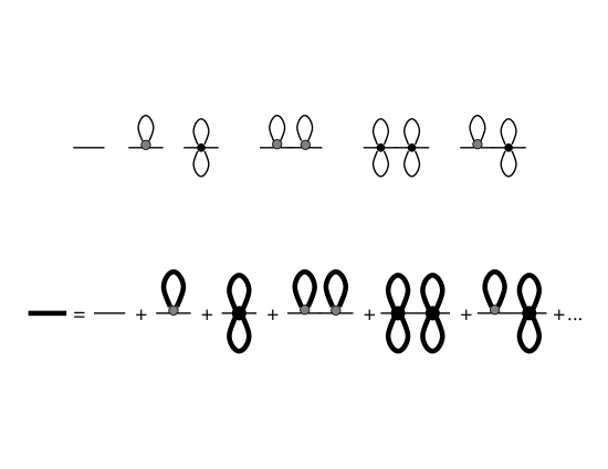
Figure 4: Top: a few diagrams contributing to the charge-charge correlation function in the one-loop Hartree approximation. Bottom: Diagrammatic representation of the self-consistent equation for the charge-charge correlation function. The thick line represents the correlation function $\tilde{G}^{H}_{\phi\phi}(k)$, thin line is the Gaussian correlation function $\tilde{G}^{0}_{\phi\phi}(k)$, the shaded circle and the bullet represent the vertices $-{\cal A}_{4}$ and $-{\cal A}_{6}$ respectively, and the ${\bf k}$-integral is associated with each loop (see also Fig.2.

$$\tilde{G}^{H}_{\phi\phi}(k)=\Bigg{[}\tilde{\cal C}^{0}_{\phi\phi}(k)+{\cal G}(\tau)\Bigg{(}\frac{{\cal A}_{4}}{2}+\frac{{\cal A}_{6}}{2^{3}}{\cal G}(\tau)\Bigg{)}\Bigg{]}^{-1}.$$

In the theory with the term $\propto\phi^{8}$ included in the effective Hamiltonian, there is another contribution, proportional to ${\cal A}_{8}{\cal G}(\tau)^{3}$, in the above equation. From the definition (66) of $\tau_{0}$ we obtain the temperature corresponding to the singularity of $\tilde{G}^{H}_{\phi\phi}(k_{b})$ at $\tau=0$ (recall that $\tilde{V}(k_{b})<0$),

$$T^{*}=-\frac{\rho_{0}^{*}\tilde{V}(k_{b})}{\Big{[}1+{\cal G}(0)\Big{(}\frac{{\cal A}_{4}}{2}+\frac{{\cal A}_{6}}{2^{3}}{\cal G}(0)\Big{)}\rho_{0}^{*}\Big{]}\big{(}1+\rho^{*}_{0}f_{2}(\rho^{*}_{0})\big{)}}.$$ (68)

The above temperature is larger from zero for ${\cal G}(0)$ assuming a finite value, for example in the RPM on the sc lattice ciach:04:1 . For ${\cal G}(0)\to\infty$, however, $T^{*}\to 0$.

In continuum there are two sources of divergency of ${\cal G}(\tau)$. The first, unphysical one is present for any $\tau$ and comes from the behavior of $\tilde{V}(k)$ for $k\to\infty$. The charge-density waves with $k\to\infty$ would correspond to overlapping hard spheres, and should not be included. Following the standard procedure brazovskii:75:0 ; fredrickson:87:0 , we expand $\Delta\tilde{V}(k)$ in a Taylor series about $k=k_{b}$ and truncate the expansion in $\Delta k=k-k_{b}$. The resulting approximate form agrees with $\tilde{G}^{H}_{\phi\phi}(k)$ for $k\approx k_{b}$, i.e. for dominant fluctuations, and its behavior for $k\to\infty$ ensures finite values of ${\cal G}(\tau)$. In the following we shall consider the integral (67) regularized as in Ref. brazovskii:75:0 ,

$${\cal G}_{r}(\tau)=\int_{\bf k}\frac{T^{*}}{\tau+\frac{V^{\prime\prime}(k_{b})}{2}\Delta k^{2}+O(\Delta k^{3})}=T^{*}k_{b}^{2}/(\pi\sqrt{2\tau\tilde{V}^{\prime\prime}(k_{b})})+...,$$ (69)

where the subscript $r$ stands for ’regularized’. Note that for reasonable regularizations (it is the neighborhood of $k_{b}$ that gives the relevant contribution to the integral) the value of ${\cal G}_{r}(\tau)$ depends on the regularization procedure only weakly (dots in the above equation).

The other, physical divergency of ${\cal G}_{r}(\tau)$ occurs only for $\tau=0$ and is associated with the singular behavior of the integrand for ${\bf k}\to{\bf k}_{b}$, i.e. with the dominant fluctuations $\tilde{\phi}({\bf k}_{b})$ ciach:04:1 . However, the temperature corresponding to $\tau\to 0$ is $T^{*}\to 0$ (see Eqs.(68) and (69)), and for $T^{*}>0$ we obtain in turn $\tau>0$, hence the charge-density correlation function $\tilde{G}^{H}_{\phi\phi}(k)$ remains regular for nonzero temperatures. Instead, a first-order transition is found for $\tau_{0}<0$ brazovskii:75:0 . In Ref.ciach:03:0 the fluctuation-induced first-order transition to the charge-ordered phase was identified with formation of an ionic crystal. The fact that the charge-density correlation function remains regular for nonzero temperatures is crucial for the occurrence of the gas-liquid type singularity in the continuum RPM.

IV.2 Critical singularity of $G_{\psi\psi}$

In this section we describe the origin of the critical singularity of $\tilde{G}_{\psi\psi}(0)$, found already in Ref. ciach:00:0 . Moreover, based on the properties of $G_{\phi\phi}$ studied in Ref.ciach:04:1 and summarized above, we show that the equation for the gas-liquid type spinodal line is well defined for any nonzero temperature.

Let us first consider the correlation functions $\langle\psi({\bf x}_{1})...\psi({\bf x}_{n})\rangle^{con}$. The higher-order contributions to the number-density correlation functions in Eq.(55) will be considered later. Contributions to the $n$-point correlation function for the field $\psi$ are given by diagrams contributing to the $2n$-point function for the field $\phi$, with $n$ pairs of external points identified, and multiplied by $a_{1}^{n}$, where $a_{1}$ is given in Eq.(54). In particular, $G_{\psi\psi}$ (Eq.(59)) is given by connected diagrams of the four-point function for the field $\phi$, with the two pairs of external points identified with each other, and multiplied by $a_{1}^{2}$. The contribution to $\tilde{G}_{\psi\psi}(0)$ leading to the critical singularity is given by an infinite series of diagrams which are of a form of chains of hyperloops connected by the vertices ${\cal A}_{4}$ ciach:00:0 (Fig.5). The sum of the corresponding geometric series has the form

$$\tilde{G}^{b}_{\psi\psi}(k)=4\tilde{g}(k)\left[1+{\cal A}_{4}\tilde{g}(k)\right]^{-1}a_{1}^{2},$$ (70)

where $\tilde{g}(k)$ is a Fourier transform of the function representing the hyperloop, i.e. a sum of all connected diagrams of the four-point function with two pairs of external points identified, which cannot be split into two distinct diagrams by splitting a single vertex ${\cal A}_{4}$ into two two-point vertices, and the sum is divided by 2 (symmetry factor). Another words, $g(r)$, represented graphically by the hyperloop in Fig.5, has no contributions which are of a form of chains. We introduced a superscript $b$ to distinguish the function given in Eq.(70) from the exact form of the correlation function defined in Eq.(59).

Eq. (70) stands a singular contribution to $\tilde{G}_{\psi\psi}$ for $k\to 0$ either when $\tilde{g}(0)\to\infty$ or when

$$1+{\cal A}_{4}\tilde{g}(0)=0.$$ (71)

The above can be satisfied for ${\cal A}_{4}<0$. Let us focus on the question for what temperatures $\tilde{g}(0)$ is regular. The lowest-order approximation for $g$ is represented by the first loop in Fig.5 (bottom), and is given by

$$\tilde{g}_{0}(k)={1\over 2}\int d{\bf r}G^{0}_{\phi\phi}(r)^{2}e^{i{\bf kr}}={1\over 2}\int d{{\bf k}^{\prime}}\tilde{G}^{0}_{\phi\phi}(k^{\prime})\tilde{G}^{0}_{\phi\phi}(|{\bf k}-{\bf k}^{\prime}|).$$ (72)

$\tilde{G}^{0}_{\phi\phi}(k)$ is nonintegrable for $\tau_{0}\to 0$, because for $\tau_{0}=0$ $\tilde{G}^{0}_{\phi\phi}(k)$ diverges sufficiently fast when $k\to k_{b}$. Thus, $\tilde{G}^{02}_{\phi\phi}(k)$ is nonintegrable as well, and for $\tau_{0}\to 0$ we have $\tilde{g}_{0}(0)\to\infty$. This singularity is associated with the charge-density waves with the wavenumber $k_{b}$.

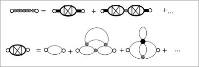
Figure 5: Top: several diagrams contributing to the correlation function $G^{b}_{\psi\psi}({\bf x}_{1},{\bf x}_{2})$, with the external points ${\bf x}_{1}\neq{\bf x}_{2}$ shown as open circles. Black boxes represent $a_{1}$. In the approximation corresponding to Eq.(70), $G^{b}_{\psi\psi}({\bf x}_{1},{\bf x}_{2})$ (represented by the pearl line) is given by an infinite series of diagrams which have a form of chains of hyperloops. Only diagrams with the hyperloops connected by the vertices ${\cal A}_{4}$ (shaded circle) are included in $G^{b}_{\psi\psi}$. Bottom: a few diagrams contributing to the hyperloop $g({\bf x}_{1},{\bf x}_{2})$. The first contribution to $g({\bf x}_{1},{\bf x}_{2})$ is $g_{0}({\bf x}_{1},{\bf x}_{2})=G^{0}_{\phi\phi}({\bf x}_{1},{\bf x}_{2})^{2}/2$.

However, the divergency of $\tilde{G}_{\phi\phi}(k_{b})$ is removed when the fluctuations are included within the Brazovskii approach described in the previous subsection. In a consistent approximation the hyperloop in Fig.5, bottom, can be written in the form

$$g^{H}({\bf x}_{1},{\bf x}_{2})=\frac{1}{2}G_{\phi\phi}({\bf x}_{1},{\bf x}_{2})^{2}+....,$$ (73)

where $G_{\phi\phi}({\bf x}_{1},{\bf x}_{2})$ is the charge-density correlation function, and dots indicate all remaining contributions. Because $\tilde{G}_{\phi\phi}({\bf k})$ is regular, $\tilde{g}^{H}(0)$ is regular as well, when the integrals are regularized for $k\to\infty$ in the way described in the preceding subsection. Thus, the only singularity of $\tilde{G}_{\psi\psi}(0)$ occurs at an infinite order in ${\cal A}_{4}$ and in this approximation is given by Eq.(71) with $g$ approximated by $g^{H}$.The function inverse to that given in Eq.(70) can be expanded about $k=0$, and we obtain

$$\tilde{C}^{b}(k)=\frac{1}{\tilde{G}^{b}_{\psi\psi}(k)}=c_{0}+c_{2}k^{2}+O(k^{4}),$$ (74)

with $c_{0}$ and $c_{2}$ expressed in terms of $\tilde{g}^{H}(0)$ and $\tilde{g}^{H^{\prime\prime}}(0)$ in a standard way. Note that the form of $\tilde{C}^{b}(k)$ for $k\to 0$ is the same as the form of the inverse Gaussian correlation function in the Landau theory for simple fluids. The above result indicates that in the perturbation theory the separation into two uniform ion-dilute and ion-dense phases is present at an infinite order in ${\cal A}_{4}$ for $c_{0}=0$. The above discussion shows that in the continuum RPM this separation is not preempted by the charge ordering.

We conclude this section by stressing that in the perturbation theory we should make a resummation of infinite series of diagrams twice. The first resummation, in the spirit of the Brazovskii theory brazovskii:75:0 , cures the artificial divergency of the charge-density correlation function in the Gaussian approximation. Critical singularity is not exhibited by any individual diagram, but by an infinite series of diagrams having the form of chains of hyperloops (Fig.5). The singularity is found only in the phase-space region where ${\cal A}_{4}<0$. Note that in the original functional $\Delta\Omega^{MF}$ (Eq.(13)) the field $\tilde{\phi}({\bf k}_{b})$ is critical, and the field $\eta$ is noncritical. Charge-density fluctuations lead to essentially different roles of both fields for ${\cal A}_{4}<0$ – the field $\phi$ is turned to be noncritical, and the field $\eta$, or in fact $\psi\propto\phi^{2}$, becomes critical.

V Universality class of the RPM critical point

In this section we separate all diagrams contributing to the vertex functions for the field $\psi$ into disjoint sets according to the rules described below. The series of diagrams in each set is given by an expression that can be represented by a secondary diagram of a skeleton form. The secondary diagrams are again segregated into disjoint sets. The series of secondary diagrams in each set can be represented by a hyperdiagram. We show that the expressions representing the hyperdiagrams are the same as the corresponding expressions representing the diagrams in a certain model system belonging to the Ising universality class. The one-to-one correspondence between the hyperdiagrams representing the vertex functions in the RPM, and the diagrams representing the vertex functions in the model belonging to the Ising universality class indicates that the singular part of the free-energy functional has the Ising universality class form, up to additional terms associated with corrections to scaling.

V.1 Secondary diagrams

In the approximation studied in the previous section $g^{H}$ can be represented by a “secondary diagram” of the same topological form as the first diagram on the r.h.s. in Fig.5, bottom, but with the thin line representing $G^{0}_{\phi\phi}({\bf x}_{1},{\bf x}_{2})$ replaced by a ’thick’ line representing $G_{\phi\phi}({\bf x}_{1},{\bf x}_{2})$, as shown in Fig.6.

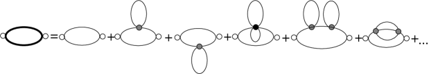
Figure 6: One-loop secondary diagram contributing to $\langle\phi^{2}({\bf x}_{1})\phi^{2}({\bf x}_{2})\rangle^{con}$ (l.h.s.), and the corresponding series of Feynman diagrams (r.h.s). Thick and thin lines represent $G_{\phi\phi}$ and $G^{0}_{\phi\phi}$ respectively, and open, gray and black circles represent external points, ${\cal A}_{4}$ and ${\cal A}_{6}$ respectively.

Similarly, all diagrams contributing to the connected correlation functions for the field $\psi({\bf x})=a_{1}\phi^{2}({\bf x})$, can be divided into disjoint sets. Each set consists of one skeleton diagram zinn-justin:89:0 and of all diagrams obtained from this skeleton by insertions for any pair of points ${\bf x}^{\prime},{\bf x}^{\prime\prime}$, connected by a thin line representing $G^{0}_{\phi\phi}({\bf x}^{\prime},{\bf x}^{\prime\prime})$, of subdiagrams which have a form of diagrams contributing to the two-point function $G_{\phi\phi}({\bf x}^{\prime},{\bf x}^{\prime\prime})$. For each set a series of all its diagrams can be represented by a secondary diagram. The secondary diagram has the same topological form as the skeleton diagram, but all lines representing $G^{0}_{\phi\phi}$ are replaced by the lines representing $G_{\phi\phi}$. In a skeleton diagram there exists no pair of lines such that by cutting only these lines a subdiagram contributing to $G_{\phi\phi}$ could be extracted. Individual secondary diagrams are regular, because $\tilde{G}_{\phi\phi}({\bf k})^{n}$ is regular and integrable when $\tilde{G}_{\phi\phi}({\bf k})$ is regularized for $k\to\infty$ as described above. In the following we shall always consider secondary diagrams. By doing so we automatically cure the divergency associated with the unphysical singularity of $\tilde{G}^{0}_{\phi\phi}({\bf k}_{b})$.

Because each vertex ${\cal A}_{2m}$ has an even number of $\phi$-legs, and in diagrams contributing to $\langle\psi({\bf x}_{1})...\psi({\bf x}_{2})\rangle^{con}$ an even number of lines representing $G_{\phi\phi}$ is connected with each external point, all diagrams contributing to $\langle\psi({\bf x}_{1})...\psi({\bf x}_{n})\rangle^{con}$ are 1PI. The secondary (skeleton) diagrams contributing to $\langle\psi({\bf x}_{1})...\psi({\bf x}_{2})\rangle^{con}$ consist of loops containing $n\geq 2$ thick lines, and the loops are connected by the vertices ${\cal A}_{2m}$ with $m\geq 2$. On the other hand, all diagrams contributing to $\langle\phi({\bf x}_{1})...\phi({\bf x}_{n})\rangle^{con}$ with ${\bf x}_{1}\neq...\neq{\bf x}_{n}$ are one particle reducible (1PR), i.e. two separate diagrams can be obtained by cutting a single line.

In the following subsections we consider vertex functions and the free-energy functional in the perturbation expansion in the vertices ${\cal A}_{2m}$. We shall segregate the corresponding secondary diagrams into different disjoint sets, associated with different contributions to the vertex functions. We focus on the general theory with ${\cal A}_{4}<0$ and ${\cal A}_{2n}>0$ for $n\geq 3$. We first analyze the lowest-order approximation.

V.2 Perturbation expansion at the zeroth-order in the vertices ${\cal A}_{2m}$ with $m\geq 3$

Let us consider diagrams that contain loops connected only by the vertices ${\cal A}_{4}$. We shall first consider a general vertex part of the form of a loop with $n\geq 3$ lines. We show that such vertex parts are negligible in the critical region, and that the free energy-functional (III.4) has the same form as in a model system described by a certain Hamiltonian of the Gaussian form.

Let us consider a general secondary diagram contributing to the $n$-th order vertex function. At the one-loop order we have

$$F^{one-loop}_{n}({\bf x}_{1},...,{\bf x}_{n})\propto G_{\phi\phi}({\bf x}_{1}-{\bf x}_{2})...G_{\phi\phi}({\bf x}_{n}-{\bf x}_{1}),$$ (75)

and the corresponding loop is shown in Fig.7.

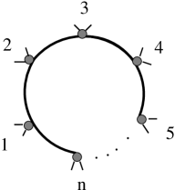
Figure 7: A loop with $n$ lines ($n\geq 3$) contributing to the $n$-point vertex function for the field $\psi$, $F_{n}({\bf x}_{1},...,{\bf x}_{n})$. Lines represent $G_{\phi\phi}$. For the above contribution we have $\int_{{\bf x}_{1}}...\int_{{\bf x}_{n}}F^{one-loop}_{n}({\bf x}_{1},...,{\bf x}_{n})\propto\tilde{G}_{\phi\phi}(0)^{n}=0$.

For $F_{n}({\bf x}_{1},...,{\bf x}_{n})$ integrated over all arguments we find at the one-loop order

$$\int_{{\bf x}_{1}}...\int_{{\bf x}_{n}}F^{one-loop}_{n}({\bf x}_{1},...,{\bf x}_{n})\propto$$

$$\int_{{\bf x}_{1}-{\bf x}_{2}}...\int_{{\bf x}_{n}-{\bf x}_{1}}G_{\phi\phi}({\bf x}_{1}-{\bf x}_{2})...G_{\phi\phi}({\bf x}_{n}-{\bf x}_{1})\propto\tilde{G}_{\phi\phi}(0)^{n}=0.$$ (76)

The last equality follows from the fact that $\tilde{G}_{\phi\phi}^{0}(0)=0$ (see Eqs.(15) and (17)), and any diagram in the perturbation expansion of $\tilde{G}_{\phi\phi}(0)$ is proportional to some power of $\tilde{G}^{0}_{\phi\phi}(0)=0$. This is because all diagrams contributing to $\tilde{G}_{\phi\phi}$ are 1PR. Note that the above property indicates short-range of the charge-density correlations in the uniform phase. For a secondary diagram with any number of loops the corresponding contribution to $\int_{{\bf x}_{1}}...\int_{{\bf x}_{n}}F_{n}({\bf x}_{1},...,{\bf x}_{n})$ is also proportional to $\tilde{G}_{\phi\phi}(0)=0$ for $n\geq 3$.

Let us consider $\Gamma_{eff}$, the generating functional for the vertex functions $F_{n}$ (see Eq.(III.4)). Because fluctuations relevant for the phase separation vary very slowly in space, let us focus on $\psi({\bf r})=\psi=const$, in which case we have

$$\beta\Gamma_{eff}[\psi]=-\int_{\bf x}F_{1}({\bf x})\psi+\frac{1}{2}\int_{{\bf x}_{1}}\int_{{\bf x}_{2}}C_{\psi\psi}(\Delta{\bf x})\psi^{2}$$

$$+\sum_{n>2}\int_{{\bf x}_{1}}...\int_{{\bf x}_{n}}\frac{F_{n}({\bf x}_{1},...,{\bf x}_{n})}{n!}\psi^{n}.$$ (77)

Let us consider the last term in the above equation. There are no zero-loop contributions to $F_{n}$ with $n\geq 3$ when the hypervertices ${\cal A}_{2m}$ with $m\geq 3$ are absent. As shown above, at a higher number of loops the last term in Eq.(V.2) vanishes, and only the first two terms remain. From the resulting form of Eq.(V.2) it follows that neglecting the hypervertices ${\cal A}_{2n}$ with $n\geq 3$ is analogous to the Gaussian approximation, provided that the fluctuations with wave numbers other than $k=0$ are disregarded. The role of the $n$-point vertex functions $F_{n}({\bf k}_{1},...,{\bf k}_{n})$, which for $k_{i}\to 0$ behave as $\propto k_{1}^{2}...k_{n}^{2}$ will be discussed in section V.5, where we briefly comment on all the irrelavant contributions to the vertex functions.

Let us determine the contribution to $G_{\psi\psi}$ coming from the secondary diagrams containing loops with more than two lines. As an example consider the secondary diagram shown in Fig.8 (top). In Fig.8 (bottom) the hyperdiagram, denoted by $f({\bf x}_{1},{\bf x}_{2})$, and obtained by a resummation of all diagrams of the above type is shown. We find

$$\int_{{\bf x}_{1}}\int_{{\bf x}_{2}}e^{i{\bf k}\cdot({\bf x}_{1}-{\bf x}_{2})}f({\bf x}_{1},{\bf x}_{2})=\tilde{f}(k)V=$$ (78)

$$\tilde{G}^{b}_{\psi\psi}(k)^{2}\tilde{G}_{\phi\phi}(k)\tilde{G}_{\phi\phi}(0)^{2}\int_{{\bf x}^{\prime}_{2}-{\bf x}^{\prime}_{3}}G^{b}_{\psi\psi}({\bf x}^{\prime}_{2}-{\bf x}^{\prime}_{3})G_{\phi\phi}({\bf x}^{\prime}_{2}-{\bf x}^{\prime}_{3})=0,$$

where we used the fact that $\tilde{G}_{\phi\phi}(0)=0$. From Eq.(78) we see that the above contribution to $\tilde{G}^{b}_{\psi\psi}(k)$ can be neglected. Similarly, all other diagrams of $\tilde{G}_{\psi\psi}(k)$, containing loops with more than two lines, are proportional to some power of $\tilde{G}_{\phi\phi}(0)=0$. Hence, when the hypervertices ${\cal A}_{2n}$ with $n>2$ are not included, the singular part of $G_{\psi\psi}$ is given by a sum of secondary diagrams of a form of a chain of loops with only two lines (Fig.9), and the inverse correlation function can be approximated by Eq.(74).

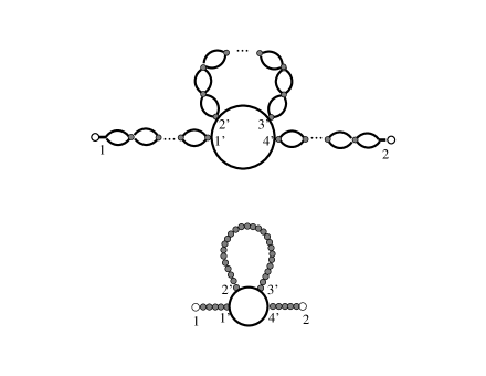
Figure 8: Top: A secondary diagram contributing to $G_{\psi\psi}$ and containing the loop of the form (75). Lines represent $G_{\phi\phi}$, gray circles represent ${\cal A}_{4}$ and black boxes connecting the external points with the loops represent $a_{1}$ (Eq.54). Bottom: A hyperdiagram obtained after a resummation of all diagrams of the form shown above. The corresponding expression in Fourier representation is given in Eq.(78)

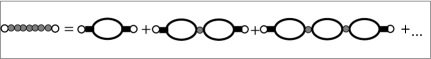
Figure 9: Secondary diagrams contributing to $G_{\psi\psi}$ (right-hand side) at the zeroth-order in the vertices ${\cal A}_{2n}$ with $n>2$. $G^{b}_{\psi\psi}$ is obtained after a resummation of all diagrams of the above form, and is represented by the pearl line. Symbols are explained in the caption of the previous figure.

At the end let us consider the one-point function, i.e. the average density. The secondary diagrams contributing to $\langle\psi({\bf x})\rangle=a_{1}\langle\phi^{2}({\bf x})\rangle$ at the zeroth order in the hypervertices ${\cal A}_{6}$ and ${\cal A}_{8}$ are shown in Fig.10, and the corresponding density shift is given by

$$\langle\psi({\bf x})\rangle=a_{1}{\cal G}_{r}(\tau)\Big{[}1-{\cal A}_{4}\tilde{g}(0)+(-{\cal A}_{4}\tilde{g}(0))^{2}+...(-{\cal A}_{4}\tilde{g}(0))^{n}\Big{]}=\tilde{G}^{b}_{\psi\psi}(0)F^{0}_{1},$$ (79)

where Eq.(67) with $G^{H}_{\phi\phi}$ replaced by $G_{\phi\phi}$, and Eq.(70) have been used, and we have introduced

$$F^{0}_{1}({\bf x})=F^{0}_{1}=\frac{{\cal G}_{r}(\tau)}{4\tilde{g}(0)a_{1}}.$$ (80)

Note that $F^{0}_{1}({\bf x})$ plays a role analogous to the external field.

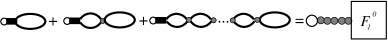
Figure 10: Diagrams contributing to the average density at the point shown as an open circle, and the hyperdiagram representing the sum of these diagrams. The black box represents $a_{1}$ (Eq.54). The pearl line represents $G^{b}_{\psi\psi}$ (Eq.(70)) and $F^{0}_{1}$ inside the box is given in Eq.(80).

The above results lead to

$$\beta\Gamma_{eff}[\psi]=-\langle F_{1}^{0}|\psi\rangle+\frac{1}{2}\langle\psi|C^{b}_{\psi\psi}|\psi\rangle,$$ (81)

where $F^{0}_{1}$ and $\tilde{C}^{b}_{\psi\psi}(k)$ are given in (80) and (74) respectively. The same form of the free-energy functional is obtained in simple fluids with the coarse-grained Hamiltonian

$$\beta{\cal H}[\psi]=\frac{1}{2}\int_{\bf k}\tilde{C}^{b}_{\psi\psi}(k)\tilde{\psi}({\bf k})\tilde{\psi}(-{\bf k})-\int_{\bf x}F^{0}_{1}\psi({\bf x})+\beta{\cal H}_{int},$$ (82)

with the term ${\cal H}_{int}$ neglected.

V.3 Even and odd secondary diagrams

The above observations indicate that the secondary diagrams contributing to the vertex functions for the field $\psi$ can be divided into two disjoint sets. In the first set, which we call the set of even diagrams, any contribution to the vertex function $F_{n}({\bf x}_{1},...,{\bf x}_{n})$ is represented by secondary diagrams such that any pair of points is either connected by an even number of lines, or is not directly connected. Such diagrams consist of chains of two-line loops, as in Fig.9 and in Figs.11-14 below. The diagrams in the other set contain loops such that there exist pairs of points connected by an odd number of lines. In particular, loops of the type shown in Fig.7, where points ${\bf x}^{\prime}$ and ${\bf x}^{\prime\prime}$ are connected by a single line representing $G_{\phi\phi}({\bf x}^{\prime}-{\bf x}^{\prime\prime})$, belong to this set of diagrams. We have shown that for $\psi$ independent of the space position such diagrams give a vanishing contribution to the free energy. In sec.5E we shall show that the odd diagrams in which some pairs of points are connected by three or more $\phi$-lines lead to a modification of the coupling constants in the corresponding coarse-grained Hamiltonian (82) and to corrections to scaling, but do not change the universality class, which is determined by the even diagrams.

Let us return to the function $g$ representing the hyperloop (see Fig.5). Note that except from the secondary diagram of the same topological form as the first diagram shown in Fig.5, bottom, all remaining secondary diagrams contributing to $g$ contain pairs of points connected by an odd number of lines and belong to the set of the odd diagrams. Hence, the approximation for $g$ given in Eq.(73) is justified as long as we limit ourseles to the set of even diagrams.

The functional (81) was obtained by a resummation of all secondary diagrams with the two-line loops connected only by the vertices ${\cal A}_{4}$. The question which arises at this point is the role of the vertices ${\cal A}_{6}$ and ${\cal A}_{8}$. For clarity of presentation we shall focus in the following subsection only on the even secondary diagrams. We shall determine the scaling behavior of the corresponding contribution to the vertex functions.

V.4 Even diagrams containing vertices ${\cal A}_{6}$ and ${\cal A}_{8}$

Let us first consider the three- and four-point vertex functions at the first order in the vertices ${\cal A}_{6}$ and ${\cal A}_{8}$, and at an arbitrary order in ${\cal A}_{4}$. If we include only even diagrams, then the associated connected correlation functions are shown in Fig.11 (left). By summing the infinite series of all diagrams of the above form we obtain the hyperdiagrams shown in Fig.11 (right).

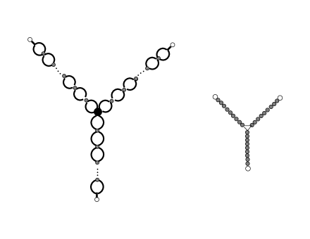
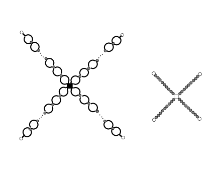
Figure 11: Top: a secondary diagram contributing to the connected three-point correlation function at the first order in ${\cal A}_{6}$ (left) and the hyperdiagram resulting from the resummation of all diagrams of the above form. Bottom: a diagram contributing to the connected four-point correlation function at the first order in ${\cal A}_{8}$ (left) and the hyperdiagram resulting from the resummation of all diagrams of the above form. The black square represents ${\cal A}_{8}$, the triangle represents the three-point vertex $F^{0}_{3}$ and the open square represents the four-point vertex $F^{0}_{4}$. The other symbols are the same as in the previous figures.

Any other secondary (i.e. of a skeleton form) diagram at the first order in ${\cal A}_{6}$ or ${\cal A}_{8}$, contributing to the respective correlation functions, belongs to the set of odd diagrams. The three- and four- point vertex functions at the first order in ${\cal A}_{6}$ and ${\cal A}_{8}$ respectively are just given by

$$\tilde{F}^{0}_{3}({\bf k}_{1},{\bf k}_{2},{\bf k}_{3})=F^{0}_{3}=\frac{{\cal A}_{6}}{a_{1}^{3}}$$ (83)

and

$$\tilde{F}^{0}_{4}({\bf k}_{1},{\bf k}_{2},{\bf k}_{3},{\bf k}_{4})=F^{0}_{4}=\frac{{\cal A}_{8}}{a_{1}^{4}}.$$ (84)

Due to the translational invariance in the real space, the Fourier transforms are defined as

$$(2\pi)^{d}\delta\big{(}\sum_{i}^{n}{\bf k}_{i})\tilde{F}_{n}({\bf k}_{1},...,{\bf k}_{n})=\int_{{\bf x}_{1}}...\int_{{\bf x}_{n}}F_{n}({\bf x}_{1},...,{\bf x}_{n})\exp\Big{(}i\sum_{j}^{n}{\bf x}_{j}{\bf k}_{j}\Big{)}.$$ (85)

The hyperdiagrams on the right in Fig.11 are of the same form as the corresponding diagrams contributing to the connected correlation functions generated by the functional (63) with the Hamiltonian (82), where

$$\beta{\cal H}_{int}=\int_{\bf r}\Bigg{(}\frac{F^{0}_{3}}{3!}\psi^{3}({\bf r})+\frac{F^{0}_{4}}{4!}\psi^{4}({\bf r})\Bigg{)},$$ (86)

when calculated at the first-order in the couplings $F^{0}_{3}$ and $F^{0}_{4}$.

At the first order in ${\cal A}_{8}$ there exists a contribution to the connected three-point correlation function of the same form as shown in Fig.11, top, left, but with the vertex ${\cal A}_{6}$ replaced by ${\cal A}_{8}{\cal G}_{r}/2$. However, the corresponding diagram belongs to the set of diagrams shown in Fig.12, left, where the number of two-line loops representing $g$ is arbitrary, from zero to infinity. Similarly, the contribution to the two-point connected correlation function with one vertex ${\cal A}_{4}$ replaced by ${\cal A}_{6}{\cal G}_{r}/2$ belongs to the set of diagrams shown in Fig.13, left, and the corresponding contribution with one vertex ${\cal A}_{4}$ replaced by ${\cal A}_{8}{\cal G}^{2}_{r}/2^{3}$ belongs to the set of diagrams shown in Fig.14, left, bottom.

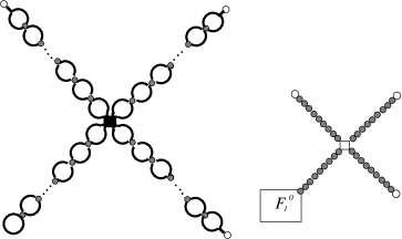
Figure 12: Left: a secondary diagram contributing to the connected three-point correlation function at the first order in ${\cal A}_{8}$ and the hyperdiagram resulting from the resummation of all diagrams of the above form. The symbols are the same as in the previous figures.

Let us consider an arbitrary vertex function for the field $\psi$, and focus on a particular contribution of a form of an even 1PI secondary diagram containing a given number of the vertices ${\cal A}_{6}$ and ${\cal A}_{8}$. Such a diagram consists of these vertices connected by chains of two-line loops, and the loops in the chain are connected by ${\cal A}_{4}$. Some of the chains of loops may end with the loop representing ${\cal G}$, as in Fig.12, left. By changing the number of loops in the chains we obtain other diagrams. All diagrams obtained in this way form a set. By a resummation of all diagrams belonging to this set we obtain a contribution to the considered vertex function, which can be represented by a hyperdiagram. The topological form of the hyperdiagram is given by any member of the set, if the chains of loops connecting the vertices ${\cal A}_{6}$ and/or ${\cal A}_{8}$ are replaced by the pearl lines, as shown in Figs.11-15.

It is instructive to consider a few examples. The even secondary diagrams contributing to $\tilde{G}_{\psi\psi}$ and containing a single vertex ${\cal A}_{6}$ and ${\cal A}_{8}$, are shown in Figs.13 and 14 (left), respectively. By summing the infinite series of all diagrams of the above form we obtain the hyperdiagrams shown in Figs.13 and 14 (right), with the pearl lines representing the ’bare’ correlation function (70). The diagrams contributing to the connected four-point function at the second order in ${\cal A}_{8}$ are shown in Fig.15.

All even secondary diagrams can be separated into disjoint sets obtained in the way described above. By a resummation of all diagrams belonging to any given set we obtain a hyperdiagram. For any hyperdiagram contributing to the vertex function in the RPM there exists a diagram of the same topological structure and representing the same expression, contributing to the vertex function in the model given by the Hamiltonian (82) and (86), and vice versa. This is just a topological property related to the possibility of connecting three- and four point vertices by lines, when the functional forms of the pearl line in the hyperdiagrams and the line in the diagrams corresponding to the above Hamiltonian are the same. We have thus reduced the question of the critical behavior of the vertex functions determined by the even diagrams to the question of the critical behavior of the system described by the Hamiltonian (82) with (86),

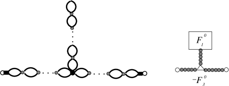
Figure 13: A diagram contributing to the number-density correlation function at the first order in ${\cal A}_{6}$ represented by the bullet (left). The contribution to $G_{\psi\psi}$, given by the infinite series of such diagrams with all numbers of hyperloops, is shown schematically (right) as a hyperdiagram, where the pearl line represents the bare function (70) and the open triangle represents $-F^{0}_{3}$(see Fig5).

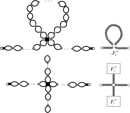
Figure 14: Left: secondary diagrams contributing to the number-density correlation function at the first order in ${\cal A}_{8}$, represented by the black square. The contributions to $G_{\psi\psi}$, given by the infinite series of such diagrams with all numbers of loops representing $g^{H}$, are shown schematically (right) as hyperdiagrams, where the pearl line represents the bare function (70) and the open square represents $-F^{0}_{4}$).

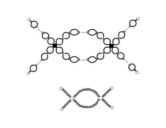
Figure 15: Top: A secondary diagram contributing to the connected four-point number-density correlation function at the second order in ${\cal A}_{8}$ (black square). Bottom: hyperdiagram representing an infinite series of all such diagrams. The pearl line represents the bare function (70).

where $\tilde{C}^{b}_{\psi\psi}(k)$, $F^{0}_{1},F^{0}_{3}$ and $F^{0}_{4}$ are given in Eqs. (74), (80), (83) and (84) respectively. We could include also higher-order vertices ${\cal A}_{2m}$ with $m>4$, and we would obtain in the same way additional terms $\propto\psi^{m}$ in Eq.(86). However, such terms are irrelevant in the RG sense amit:84:0 ; zinn-justin:89:0 .

By shifting the field,

$$\psi=\varphi-\frac{F^{0}_{3}}{F^{0}_{4}},$$ (87)

we can remove the term $\propto\psi^{3}$ in Eq.(86), and we obtain the standard form of the coarse-grained Hamiltonian representing the Ising universality-class, ${\cal H}[\psi]/c_{2}={\cal H}^{I}[\varphi]+const.$, with ${\cal H}^{I}[\varphi]$ given in Eq.(20), where the two relevant scaling fields are

$$H_{0}=\Bigg{(}F^{0}_{1}+\frac{F^{0}_{3}}{F^{0}_{4}}c_{0}-\frac{F^{03}_{3}}{3F^{02}_{4}}\Bigg{)}c_{2}^{-1}$$ (88)

and

$$t_{0}=\Bigg{(}c_{0}-\frac{F^{02}_{3}}{2F^{0}_{4}}\Bigg{)}c_{2}^{-1},$$ (89)

and $u_{0}=F^{0}_{4}c_{2}^{-1}$. Note that the scaling fields $H_{0}$ and $t_{0}$ are related to the temperature and the chemical potential (through $\rho_{0}^{*}$) in a somewhat complex way. Moreover, the values of the above parameters depend on ${\cal G}_{r}$ and $\tilde{g}(k)$, which in turn depend on the regularization procedure of the ${\bf k}$-integrals of $\tilde{G}_{\phi\phi}$ and its powers. We shall not study the nonuniversal properties in this work.

The contributions of all even diagrams to the vertex functions for the field $\psi$ are of the same form as the vertex functions determined by the Hamiltonian given in Eq.(20) and belonging to the Ising universality class. Hence, the scaling properties are also the same. We need to find out whether the odd-diagrams contributions to the vertex functions can alter the scaling properties.

V.5 Odd diagrams containing vertices ${\cal A}_{6}$ and ${\cal A}_{8}$

In this section we consider the secondary diagrams contributing to the vertex functions for the field $\psi\propto\phi^{2}$, in which there exist pairs of points connected by an odd number of lines representing $G_{\phi\phi}$. We focus on the theory with the vertices ${\cal A}_{4}<0$ and ${\cal A}_{2n}>0$ for $n\geq 3$. Our purpose is to show that the odd diagrams give the contributions to the vertex functions which either scale in the same way as the even diagrams, or are associated with corrections to scaling. Because an even number of the $\phi$-lines emanates from each vertex and each external point, and an even number of lines is amputated from the external points in diagrams contributing to the vertex functions for $\psi$, the vertices connected by an odd number of lines form closed loops.

V.5.1 Irrelavant odd diagrams

In sec.5.B we have already considered loops formed by single lines, as shown in Fig.7, where $\tilde{F}_{n}({\bf k}_{1},...{\bf k}_{n})\propto\prod_{i}^{n}\tilde{G}_{\phi\phi}(k_{i})\propto k_{1}^{2}...k_{i}^{2}...k_{n}^{2}$ for $k_{i}\to 0$. Let us focus on a contribution to $\tilde{F}_{n}({\bf k}_{1},...{\bf k}_{n})$ that is of the form $\tilde{F}^{odd}_{\{j_{i}\}}({\bf k}_{1},...{\bf k}_{n})\propto k_{1}^{2j_{1}}...k_{i}^{2j_{i}}...k_{n}^{2j_{n}}$, where $j_{i}=0,1$ and $\sum_{i}j_{i}>0$, and in the corresponding secondary diagrams no pair of points is connected only by a chain of the two-line $g$-loops, and no loops representing ${\cal G}$ are present. A series of such secondary diagrams for a given $\{j_{i}\}$ can be represented by a hyperdiagram containing no pearl lines. We have $\int_{{\bf x}_{1}}...\int_{{\bf x}_{n}}F_{\{j_{i}\}}^{odd}({\bf x}_{1},...{\bf x}_{n})=0$, because $\sum_{i}j_{i}>0$.

By following the considerations described in the preceding subsection, we can segregate all secondary diagrams contributing to a particular vertex function into disjoint sets. In the secondary diagrams belonging to each set the vertices ${\cal A}_{6}$, ${\cal A}_{8}$ and $F_{\{j_{i}\}}^{odd}$ are connected by the chains of the two-line $g$-loops. All diagrams in any given set are of the same topological structure, when the chains of the two-line loops are replaced by the pearl lines. The series of all diagrams in the given set is represented by a hyperdiagram. There is a one-to-one correspondence between the hyperdiagrams described above, and diagrams obtained in the perturbation expansion in the theory with the coarse-grained Hamiltonian (82) and with ${\cal H}_{int}$ (86) supplemented with contributions of the form $O(\psi)\propto\int_{{\bf k}_{1}}...\int_{{\bf k}_{n}}\delta(\sum_{i}^{n}{\bf k}_{i})\prod_{i}^{n}\tilde{\psi}({\bf k}_{i})k_{i}^{2j_{i}}$ with $n\geq 3$. Note, however that in the critical region the terms $O(\psi)$ correspond to irrelevant operators in the RG sense zinn-justin:89:0 .

V.5.2 Relevant odd secondary diagrams

Let us consider odd secondary diagrams contributing to the vertex functions for the field $\psi$, other than those proportional to $\tilde{G}_{\phi\phi}(0)=0$, which are irrelevant. In such diagrams there exist closed loops in which neighboring pairs of points, ${\bf x}_{1}$ and ${\bf x}_{2}$, are connected by subdiagrams contributing to $G_{3}({\bf x}_{1}-{\bf x}_{2})=\langle\phi^{3}({\bf x}_{1})\phi^{3}({\bf x}_{2})\rangle$. The diagrams contributing to $G_{3}({\bf x}_{1}-{\bf x}_{2})$ are shown in Fig.16.

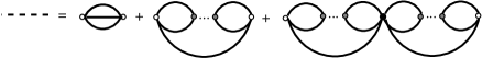
Figure 16: Relevant odd secondary diagrams contributing to the correlation function $G_{3}({\bf x}_{1},{\bf x}_{2})=\langle\phi^{3}({\bf x}_{1})\phi^{3}({\bf x}_{2})\rangle$. The dashed line represents the series of all diagrams of the form shown on the r.h.s.

Because $\tilde{G}_{\phi\phi}(k)\sim k^{2}$ for $k\to 0$, and the integrals are regularized for $k\to\infty$ as described in sec.4, the individual diagrams contributing to $\tilde{G}_{3}(0)$ are finite. The series of diagrams of the form shown in the second diagram on the r.h.s. in Fig.15 is also regular for the same reason. In the theory with ${\cal A}_{6}>0$ the series of all diagrams shown on the r.h.s. in Fig.15 is regular for $k\to 0$, and we find $\tilde{G}_{3}(k)=g_{3}^{0}+g_{3}^{2}k^{2}+...$. Note the significant difference between the pearl line (Fig.9) obtained after the resummation of the even diagrams, and the dashed line obtained after the resummation of the odd diagrams (Fig.16). Because ${\cal A}_{4}<0$ and ${\cal A}_{6}>0$, only the pearl line can be singular for $k\to 0$.

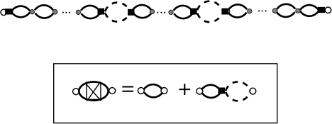
Figure 17: Top: Relevant odd secondary diagram contributing to the two-point correlation function for the field $\psi$. The dashed lines represent the sum over all subdiagrams contributing to $G_{3}$, and the solid lines represent $G_{\phi\phi}$. The gray circles, black squares, open circles and black boxes represent ${\cal A}_{4}$, ${\cal A}_{8}$, the external points, and $a_{1}$ respectively. Bottom: secondary diagrams contributing to the hyperloop representing $g$, when the even as well as the relevant odd diagrams are included, and the vertices ${\cal A}_{2m}$ with $m>4$ are neglected.

In Fig.17, top, we show a relevant odd secondary diagram contributing to the two-point correlation function for the field $\psi$. This diagram represents in fact the series of all secondary diagrams that contain subdiagrams contributing to $G_{3}({\bf x}-{\bf x}^{\prime})$ for each pair of the vertices ${\bf x}$ and ${\bf x}^{\prime}$ connected by the dashed line in Fig.17. We shall keep the name ’a secondary diagram’ for such a series of secondary diagrams. The corresponding secondary diagrams contributing to the hyperloop $g$ (see sec.IVB, Fig.5) are shown in Fig.17, bottom, where the irrelevant diagrams are not included. In this approximation we obtain for $\tilde{G}^{b}_{\psi\psi}(k)$ the same expression as given in Eq.(70), but with $\tilde{g}(k)$ given by

$$\tilde{g}(k)=\tilde{g}^{H}(k)\Big{(}1+\frac{{\cal A}_{8}}{2}\int_{\bf x}G_{3}({\bf x})^{2}e^{i{\bf k}{\bf x}}\Big{)},$$ (90)

where $g^{H}$ is given in Eq.(73), and $G_{3}$ is shown in Fig.16. For $k\to 0$ we obtain the bare two-point correlation function $\tilde{G}^{b}_{\psi\psi}(k)$ of the same form as given in Eq.(74), but with modified coefficients $c_{0}$ and $c_{2}$. Note that the secondary diagrams contributing to the bare function $\tilde{G}^{b}_{\psi\psi}(k)$ contain vertices other than ${\cal A}_{4}$, unlike in the case of the even diagrams. Note also that the secondary diagrams which contain chains of loops such that the two ends of the chain emerge from the same vertex, or one end of the chain represents ${\cal G}(\tau)$ (as is the case in Fig.14), are not included in the bare function $G^{b}_{\psi\psi}$. As in the case of the even secondary diagrams, only linear chains, with no chain-like branches, contribute to $G^{b}_{\psi\psi}$.

Figure 18: Relevant odd secondary diagram contributing to the $n$-point vertex function for the field $\psi$. The black squares represent ${\cal A}_{8}$. The dashed line represents the three-point correlation function $G_{3}$. Thin lines represent the (amputated) $\phi$-lines.

In Fig.18 we show the contribution to the $n$-point vertex function for the field $\psi$, $\tilde{F}^{odd}_{n}({\bf k}_{1},...,{\bf k}_{n})$, of the form $\prod_{i}\tilde{G}_{3}(k_{i})$. Note that $\tilde{G}_{3}(k)=g^{0}_{3}+g^{2}_{3}k^{2}+O(k^{4})$ is finite for $k\to 0$, therefore the above contribution to $\tilde{F}^{odd}_{n}({\bf 0},...,{\bf 0})$, being of the form $\propto\tilde{G}_{3}(0)^{n}$, is nonvanishing as well. Hence, the above contribution to $\tilde{F}_{n}$ is relevant in the critical region, and should be taken into account. By $\tilde{F}^{0odd}_{n}({\bf k}_{1},...,{\bf k}_{n})=F^{0odd}_{n}+O(k^{2})$ we denote the contribution to $\tilde{F}^{odd}_{n}({\bf k}_{1},...,{\bf k}_{n})$ which is given by all odd secondary diagrams such that no pair of vertices is connected only by a chain of the $g$-hyperloops and no loops representing ${\cal G}$ are present. The vertex part $\tilde{F}^{0odd}_{n}({\bf 0},...,{\bf 0})=F^{0odd}_{n}$ is relevant in the critical region, and $F^{0odd}_{n}$ should be taken into account in the same way as the vertices ${\cal A}_{2n}$ are. Thus, the contributions to any vertex function, which are relevant in the critical region, consist of the even secondary diagrams, as well as of the relevant odd secondary diagrams (those which contain the dashed lines). Any relevant 1PI secondary diagram contains vertices ${\cal A}_{6}$, ${\cal A}_{8}$ and the vertex parts $F^{0odd}_{3}$, $F^{0odd}_{4}$, from which there emanate 3 or 4 linear chains of hyperloops respectively, and the chains are of the form shown in Fig.17. An example of an odd secondary diagram contributing to the four-point connected correlation function is shown in Fig.19.

As in the case of the even diagrams, we can segregate all the relevant diagrams (both even and odd) into disjoint sets. To a given set there belongs a diagram in which particular pairs of vertices or the vertex parts are connected by the linear chains of the hyperloops. All secondary diagrams obtained from this particular diagram by changing the number of the hyperloops in the chains belong to the same set. This is analogous to the segregation of the even diagrams described in sec.VD.

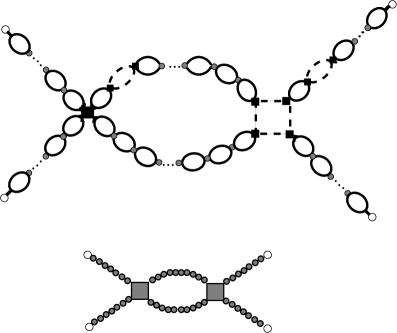
Figure 19: Top: A relevant odd secondary diagram contributing to the four-point connected correlation function for the field $\psi$. The gray circles, black squares, open circles and black rectangles represent ${\cal A}_{6}$, ${\cal A}_{8}$, external points, and $a_{1}$ respectively. The solid and dashed lines represent the two- and the three-point correlation functions for the field $\phi$, $G_{\phi\phi}$ and $G_{3}$ respectively. All diagrams obtained by changing the number of the solid- and the dashed-line loops in the four linear chains belong to the same set of diagrams. Bottom: A hyperdiagram obtained after the resummation over all numbers $n\geq 1$ of the solid-line loops and over $0\leq m\leq n-1$ dashed-line loops in each linear chain, and over all subdiagrams contributing to the bare four-point vertex functions. The pearl-line represents the series of all linear chains and the bare four-point vertex functions are represented here as the shaded squares. See text for more datails.

There is one-to-one correspondence between the vertex functions in our theory and the vertex functions obtained in the theory with the coarse-grained Hamiltonian (82), when the terms

$$\frac{1}{3!}\int_{{\bf k}_{1}}...\int_{{\bf k}_{3}}(2\pi)^{d}\delta(\sum_{i}^{3}{\bf k}_{i})\tilde{F}^{0odd}_{3}({\bf k}_{1},...,{\bf k}_{3})\prod_{i}^{3}\tilde{\psi}({\bf k}_{i})$$ (91)

and

$$\frac{1}{4!}\int_{{\bf k}_{1}}...\int_{{\bf k}_{4}}(2\pi)^{d}\delta(\sum_{i}^{4}{\bf k}_{i})\tilde{F}^{0odd}_{4}({\bf k}_{1},...,{\bf k}_{4})\prod_{i}^{4}\tilde{\psi}({\bf k}_{i})$$ (92)

are added to ${\cal H}_{int}$ (Eq.(86)). Because of the form of $\tilde{F}^{0odd}_{n}({\bf k}_{1},...,{\bf k}_{n})$, we can separate the relevant contributions,

$$\frac{F^{0odd}_{3}}{3!}\int_{{\bf k}_{1}}...\int_{{\bf k}_{3}}(2\pi)^{d}\delta(\sum_{i}^{3}{\bf k}_{i})\prod_{i}^{3}\psi({\bf k}_{i})=\frac{F^{0odd}_{3}}{3!}\int_{{\bf x}}\psi({\bf x})^{3}$$ (93)

and

$$\frac{F^{0odd}_{4}}{4!}\int_{{\bf k}_{1}}...\int_{{\bf k}_{4}}(2\pi)^{d}\delta(\sum_{i}^{4}{\bf k}_{i})\prod_{i}^{4}\tilde{\psi}({\bf k}_{i})=\frac{F^{0odd}_{4}}{4!}\int_{{\bf x}}\psi({\bf x})^{4}.$$ (94)

In the remaining contributions the integrands are proportional to $O(k_{i}^{2})$ for $k_{i}\to 0$. Such contributions to ${\cal H}_{int}$ are irrelevant in the RG sense zinn-justin:89:0 . The vertex functions for the field $\psi$ scale in the same way as the vertex functions in the model given by the Hamiltonian (82) and (86), but with all the parameters modified according to the above discussion. In particular, $F^{0}_{n}\rightarrow{\cal A}_{n}/a_{1}^{n}+F^{0odd}_{n}$.

With higher-order vertices ${\cal A}_{2m}$, $m>4$ included, similar vertex parts with loops made of subdiagrams contributing to $\langle\phi^{5}({\bf x}_{1})\psi^{5}({\bf x}_{2})\rangle^{con}$ etc. would contribute to $F^{0}_{3}$, $F^{0}_{4}$ in Eq. (86), and to the irrelevant operators. Modification of the coupling constants affects only the nonuniversal properties of the theory. Corrections to scaling associated with irrelevant operators have been studied before zinn-justin:89:0 , and are not specific for the RPM.

Let us summarize the above results. From all the secondary diagrams contributing to the vertex function for the field $\psi$, $\tilde{F}_{n}({\bf k}_{1},...,{\bf k}_{n})$, we can distinguish a set of secondary diagrams contributing to the ’bare’ $n$-point vertex function. To the above set there belong the vertex ${\cal A}_{2n}/a_{1}^{n}$ and the odd secondary diagrams such that no pair of vertices ${\cal A}_{2m}$ is connected by the linear chain of the hyperloops representing $g$ (including the one-loop chains representing $g^{H}$). Also, no loops representing ${\cal G}$ are present in the diagrams contributing to the bare vertex function. The bare vertex function has the form $\tilde{F}^{bare}_{n}({\bf k}_{1},...,{\bf k}_{n})={\cal A}_{2n}/a_{1}^{n}+F^{0odd}_{n}+O(k^{2})$ for $k\to 0$, where $F^{0odd}_{n}$ is a real number. The remaining secondary diagrams contributing to the vertex function $\tilde{F}_{m}({\bf k}_{1},...,{\bf k}_{m})$ consist of the subdiagrams of the form described above, and these subdiagrams are connected by the chains of the hyperloops representing $g$ (including the one-loop chains representing $g^{H}$). All the secondary diagrams contributing to the $n$-point vertex function for the field $\psi$ can be segregated into disjoint sets. Each set contains all the secondary diagrams obtained from one particular secondary diagram by changing the number of the hyperloops in the chains connecting the subdiagrams that belong to the set representing the bare vertex functions. Also the secondary diagrams obtained from the chosen diagram by changing the subdiagrams that contribute to the bare vertex functions belong to the considered set. All the secondary diagrams in any given set are of the same topological structure when the linear chains are replaced by lines, and the subdiagrams contributing to the bare $n$-point vertex function are replaced by vertices from which $n$ lines emanate. The series of all the secondary diagrams in a given set can be represented by a hyperdiagram. The hyperdiagram has the same topological structure as the secondary diagrams in the set. In the hyperdiagrams the functional form of the line representing the sum over all numbers of the hyperloops in the linear chain is $1/(c_{0}+c_{2}k^{2})$ in Fourier representation, and the $n$-point hypervertices are of the form ${\cal A}_{2n}/a_{1}^{n}+F^{0odd}_{n}+O(k^{2})$ for $k\to 0$. The generating functional for such vertex functions is obtained from the Hamiltonian (82) with (86), that contains also additional, irrelevant contributions to ${\cal H}_{int}$ that yield corrections to scaling.

V.6 Corrections to scaling specific for the RPM

We found that the connected correlation functions for the field $\psi$ scale in the same way as in the Ising universality class. However, the correlation functions for the number-density, given in Eq.(55), contain also other contributions. In particular, the one- and two-point number-density correlation functions in the RPM assume the forms

$$\langle\eta({\bf r})\rangle=\langle\psi({\bf r})\rangle+\sum_{n\geq 1}\frac{a_{n}}{a_{1}^{n}n!}\langle\psi^{n}({\bf r})\rangle^{con}$$ (95)

and

$$\langle\eta({\bf r}_{1})\eta({\bf r}_{2})\rangle^{con}=\langle\psi({\bf r}_{1})\psi({\bf r}_{2})\rangle^{con}+\sum_{n,m\geq 1}\sum_{n+m>2}\frac{a_{n}a_{m}}{a_{1}^{n+m}n!m!}\langle\psi^{n}({\bf r}_{1})\psi^{m}({\bf r}_{2})\rangle^{con}$$ (96)

respectively, where the averages are obtained with the Hamiltonian (34). In Figs.20 and 21 we show the secondary diagrams contributing to the next-to-leading order terms in the above expansions. On the right the hyperdiagrams obtained after the resumation of all such diagrams are shown.

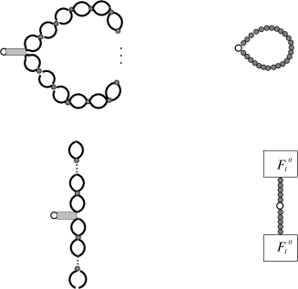
Figure 20: Left: Secondary diagrams contributing to the next-to-leading order term in the expansion of $\langle\zeta({\bf r})\rangle$ (Eq.(95)) at the zeroth order in the hypervertices ${\cal A}_{2n}$ with $n>2$. The external point is shown as an open circle, gray boxes represent $a_{2}/2$, lines represent $G_{\phi\phi}$ and gray circles represent ${\cal A}_{4}$. Right: Hyperdiagrams resulting from the resummation of all diagrams of the type shown on the left.

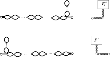
Figure 21: Left: secondary diagrams contributing to the next-to-leading order term in the expansion of $G_{\zeta\zeta}$ (Eq.(96)) at the zeroth order in the hypervertices ${\cal A}_{n}$ with $n>4$. The external points are shown as open circles. black and gray boxes represent $a_{1}$ and $a_{2}/2$ repsectively, lines represent $G_{\phi\phi}$ and gray circles represent ${\cal A}_{4}$. Right: Hyperdiagrams resulting from the resummation of all diagrams of the type shown on the left.

In general, the leading-order correction to the $N$-point connected correlation function for the field $\psi$ is given by the $N+1$-point connected correlation function, where two of the external points are identified. Scaling forms of the connected correlation functions, Eq. (21), give

$$G^{R}_{N}({\bf r}_{1},...,{\bf r}_{N};t,u,H)=|t|^{N\beta}G_{Ns}({\bf r}_{1}/\xi,...,{\bf r}_{N}/\xi;H|t|^{-\Delta})+$$ (97)

$$|t|^{(N+1)\beta}G_{(N+1)s}({\bf r}_{1}/\xi,{\bf r}_{1}/\xi,...,{\bf r}_{N}/\xi;H|t|^{-\Delta})+O(|t|^{(N+2)\beta}),$$

where $G_{Ns}({\bf r}_{1}/\xi,...,{\bf r}_{N}/\xi;H|t|^{-\Delta})$ is the scaling function. Consider now the correction term to the grand potential. Because the relative correction to any connected correlation function is $\propto|t|^{\beta}$, the relative correction to their generating functional has the same scaling form, and we obtain

$$\Omega(t,H)=|t|^{2-\alpha}\Big{[}\omega_{s}(H|t|^{-\Delta})+|t|^{\beta}\omega_{cs}(H|t|^{-\Delta})+...\Big{]}.$$ (98)

All derivatives of the grand potential can be written in the form

$$X\propto|t|^{a}\Big{[}1+|t|^{\beta}X_{cs}(H|t|^{-\Delta})+O(|t|^{2\beta})\Big{]},$$ (99)

where $a$ is the corresponding critical parameter in the Ising universality class. The leading-order correction to scaling, specific for the RPM, is given by the exponent $\beta$.

VI summary

The theory outlined above is relatively complex compared to the theory of critical phenomena in simple systems. This complexity follows from the indirect nature of criticality in ionic systems. The long-range critical number-density fluctuations in charged systems are not induced by mechanical interactions. Unlike in systems with short-range interactions, the phase separation is induced by strong charge-density correlations. Coulombic forces support formation of charge-ordered structures with a microscopic distance between oppositely charged neighbors. Individual microscopic states are charge-ordered with a high probability as predicted theoretically ciach:01:0 and seen in snapshots weis:98:0 ; panag:02:0 ; yan:02:0 , but fluctuations restore the uniform structure at larger length scales (and large observation times). Mathematically the restored disorder is described within the Brazovskii approach. In our case we performed a resummation of singular Feynman diagrams (singularity resulting from charge-ordering) to obtain regular secondary diagrams. The charge-ordered ’living’ clusters that are formed in different microstates interact with each other with short-range forces, and this observation suggests standard criticality. In microscopic description interactions between clusters of various sizes, shapes and orientations should be considered. The above complexity in our theory is reflected in the absence of critical singularity in individual secondary diagrams. The critical instability of the uniform phase occurs only when an infinite series of secondary diagrams contributing to the correlation function $\langle\phi^{2}({\bf x}_{1})\phi^{2}({\bf x}_{2})\rangle^{con}$ is calculated in the perturbation expansion. In the diagrams of a form of chains of $n$ loops the correlations with $n-1$ intermediate points are included. The series of chains of loops plays an analogous role as the Gaussian correlation function in simple fluids. The hyperdiagrams with the lines representing such series play in turn an analogous role as diagrams in the standard theory of critical phenomena.

From the point of view of the field theory, the above work concerns the theory with the action of the form (34) with ${\cal A}_{4}<0$ and ${\cal A}_{2n}>0$ for $n>3$, and in Fourier space the action becomes unstable for the wavenumber $k_{b}\neq 0$. The key properties ${\cal A}_{4}<0$ and ${\cal A}_{2n}>0$ have been observed within the WF approximation at low densities for the RPM with the ideal entropy of mixing ciach:04:1 and with the Percus-Yevick patsahan:05:0 reference system. It is plausible that for the exact form of ${\cal A}_{4}$ the condition ${\cal A}_{4}<0$ is satisfied in the RPM for low densities, but it remains to be proven. This work shows that the model for which the above is satisfied belongs to the Ising universality class.

- (1) G. Stell, K. Wu, and B. Larsen, Phys. Rev. Lett. 37, 1369 (1976).
- (2) B. Hafskjold and G.Stell, in The Liquid State of matter. Fluids, Simple and Complex, edited by E. Montroll and J. Lebowitz (North Holland, Amsterdam, 1982).
- (3) G. Stell, Phys. Rev. A 45, 7628 (1992).
- (4) G. Stell, J. Stat. Phys. 78, 197 (1995).
- (5) A. Ciach and G. Stell, J. Mol. Liq. 87, 253 (2000).
- (6) A. Ciach and G. Stell, Physica A 306, 220 (2002).
- (7) A. Ciach and G. Stell, Int.J. Mod. Phys. B 21, 3309 (2005).
- (8) M. L. Japas and J. M. H. Levelt-Sengers, J. Phys. Chem. 94, 5361 (1990).
- (9) T. Narayanan and K. S. Pitzer, J. Phys. Chem. 98, 9170 (1994).
- (10) K. S. Pitzer, Acc. Chem. Res. 23, 373 (1990).
- (11) R. R. Singh and K. S. Pitzer, J. Chem. Phys. 92, 6775 (1990).
- (12) K. C. Zhang, M. E. Briggs, R. W. Gammon, and J. M. H. Levelt-Sengers, J. Chem. Phys. 97, 8692 (1992).
- (13) H. Weingärtner and W. Schröer, Adv. Chem. Phys 116, 1 (2001).
- (14) H. L. Bianchi and M. L. Japas, J. Chem. Phys. 115, 10472 (2001).
- (15) M. Anisimov et al., Phys. Rev. Lett. 85, 2336 (2000).
- (16) R. Dickman and G. Stell, in Simulation and theory of electrostatic interactions in solution, edited by L. Pratt and G. Hummer (AIP Conf. Proceedings 492, Melville, NY, 1999).
- (17) A. Z. Panagiotopoulos and S. Kumar, Phys. Rev. Lett. 83, 2981 (1999).
- (18) A.Diehl and A.Z.Panagiotopoulos, J. Chem. Phys. 118, 4993 (2003).
- (19) J. Hoye and G. Stell, J. Stat. Phys. 89, 177 (1997).
- (20) G. Stell, in New Approaches to Problems in Liquid-State Theory, edited by C. Caccamo, J.-P. Hansen, and G. Stell (Kluwer Academic Publishers, Dordrecht, 1999).
- (21) A. Ciach and G. Stell, J. Chem. Phys. 114, 3617 (2001).
- (22) V. Kobelev, A. B. Kolomeisky, and M. Fisher, J. Chem. Phys. 117, 8897 (2002).
- (23) A.Brognara, A. Parola, and L. Reatto, Phys. Rev. E 65, 66113 (2002).
- (24) M. E. Fisher, J. Stat. Phys. 75, 1 (1994).
- (25) S. Wiegand et al., Int. J. Thermophys. 15, 1045 (1994).
- (26) S. Wiegand et al., J. Chem. Phys. 106, 2777 (1997).
- (27) S. Wiegand et al., J. Chem. Phys. 109, 9038 (1998).
- (28) S. Wiegand, R. F. Berg, and J. M. Levelt-Sengers, J. Chem. Phys. 109, 4533 (1998).
- (29) M. Kleemeier, S. Wiegand, W. Schröer, and H. Weingärtner, J. Chem. Phys. 110, 3085 (1999).
- (30) M. Wagner, O. Stanga, and W. Schröer, PCCP 4, 5300 (2002).
- (31) M. Wagner, O. Stanga, and W. Schröer, PCCP 5, 3943 (2003).
- (32) M. Wagner, O. Stanga, and W. Schröer, PCCP 6, 580 (2004).
- (33) A. F. Kostko, M. A. Anisimov, and J. V. Sengers, Phys. Rev. E 70, 026118 (2004).
- (34) G. Orkoulas and A. Z. Panagiotopoulos, J. Chem. Phys. 110, 1581 (1999).
- (35) Q. Yan and J. J. de Pablo, J. Chem. Phys. 111, 9509 (1999).
- (36) E. Luijten, M. Fisher, and A. Panagiotopoulos, J. Chem. Phys. 114, 5468 (2001).
- (37) J.-M. Caillol, D. Levesque, and J.-J. Weis, J. Chem. Phys. 116, 10794 (2002).
- (38) E. Luijten, M. Fisher, and A. Panagiotopoulos, Phys. Rev. Lett. 88, 185701 (2002).
- (39) Y. C. Kim, M. E. Fisher, and E. Luijten, Phys. Rev. Lett. 91, 065701 (2003).
- (40) D. J. Amit, Field Theory, the Renormalization Group and Critical Phenomena (World Scientific, Singapore, 1984).
- (41) Zinn-Justin, Quantum Field Theory and Critical Phenomena (Clarendon Press, Oxford, 1989).
- (42) A. Ciach, W. T. Gozdz, and G. Stell, cond-mat/0411424 .
- (43) S. A. Brazovskii, Sov. Phys. JETP 41, 8 (1975).
- (44) A. Ciach, Phys. Rev. E 70, 046103 (2004).
- (45) A. Ciach and G. Stell, Phys. Rev. Lett. 91, 60601 (2003).
- (46) A. Ciach and G. Stell, Phys. Rev. E 70, 16114 (2004).
- (47) A. Diehl and A. Z. Panagiotopolous, Phys. Rev. E 71, 046118 (2005).
- (48) G. H. Fredrickson and E. Helfand, J. Chem. Phys. 87, 67 (1987).
- (49) A. Ciach and G. Stell, J. Chem. Phys. 114, 382 (2001).
- (50) J.-J. Weis, D. Levesque, and J. Caillol, J. Chem. Phys. 109, 7486 (1998).
- (51) A. Panagiotopoulos and M. Fisher, Phys. Rev. Lett. 88, 45701 (2002).
- (52) Q. Yan and J. de Pablo, Phys. Rev. Lett. 88, 95504 (2002).
- (53) O. Patsahan and A. Ciach, , to be published.