Sensitivity and back-action in charge qubit measurements by a strongly coupled single-electron transistor

Abstract

We consider charge-qubit monitoring (continuous-in-time weak measurement) by a single-electron transistor (SET) operating in the sequential-tunneling régime. We show that commonly used master equations for this régime are not of the Lindblad form that is necessary and sufficient for guaranteeing valid physical states. In this paper we derive a Lindblad-form master equation and a corresponding quantum trajectory model for continuous measurement of the charge qubit by a SET. Our approach requires that the SET-qubit coupling be strong compared to the SET tunnelling rates. We present an analysis of the quality of the qubit measurement in this model (sensitivity versus back-action). Typically, the strong coupling when the SET island is occupied causes back-action on the qubit beyond the quantum back-action necessary for its sensitivity, and hence the conditioned qubit state is mixed. However, in one strongly coupled, asymmetric régime, the SET can approach the limit of an ideal detector with an almost pure conditioned state. We also quantify the quality of the SET using more traditional concepts such as the measurement time and decoherence time, which we have generalized so as to treat the strongly responding régime.

I Introduction

The single-electron transistorAverin and Likharev (1986); Fulton and Dolan (1987) (SET) has been suggestedShnirman and Schön (1998); Devoret and Schoelkopf (2000) as a device to measure the state of charge qubits, one proposal for the fundamental elements of a quantum computer.Nielsen and Chuang (2000) In solid-state systems it is well known that realistic measurement devices such as the SET and quantum point contactField et al. (1993) (QPC) do not perform instantaneous measurements. Rather, it is necessary to treat the measurement as a sequence of weak measurements, resulting in a continuous process in time.

During such a continuous measurement, the conditioned qubit state is gradually projected into an eigenstate in the measurement basis. Here the conditioned state is one that an experimenter would calculate knowing the output of the detector. On average (that is, ignoring this information) the effect of the measurement is simply to decohere (that is, remove the coherences of) the qubit in the measurement basis. This quantum back-action is unavoidable because the coherences between the eigenstates (which indicate that the qubit is in a superposition of these eigenstates) must vanish for one or the other eigenstate to be realized. For an idealKorotkov (1999) or quantum-limitedBraginsky and Khalili (1992) detector, the decoherence is equal to the minimum back-action allowed by quantum mechanics given the information obtained from the detector. Consequently, a qubit state conditioned upon the output of an ideal detector would remain pure if it began pure. This is the case for the usual model of the QPC.Gurvitz (1997); Korotkov (1999); Goan et al. (2001)

In this paper we maintain the purity of the conditioned state as the ultimate quantifier of the quality of the measurement. However, it has been common to use a different quantifier, namely a comparison between the decoherence rate $\Gamma_{\rm d}$ and the measurement rate $\tau^{-1}_{\rm m}$. These are the characteristic rates of the decoherence and the measurement (gradual projection) processes discussed above. (It is assumed that there is only one characteristic rate). For so-called “weakly responding”Korotkov (1999) detectors, the ratio of these rates is limited byDevoret and Schoelkopf (2000)

$$\Gamma_{\rm d}\tau_{\rm m}\geq\frac{1}{2},$$ (1)

with equality implying an ideal detector. While not the main focus of this paper, we show that in general the detector quality cannot be captured by such a simple ratio, which is sometimes referred to as the detector efficiency.Pilgram and Büttiker (2002) For example, for a QPC it is easy to verify that $\Gamma_{\rm d}\tau_{\rm m}$ varies between 1 (in the strong-response limit) and 1/2 (in the weak-response limit). This is discussed in Appendix A.

To date, theoretical treatmentsShnirman and Schön (1998); Makhlin et al. (2000); Korotkov (2001); Makhlin et al. (2001, 2002) of charge-qubit continuous measurements by SETs operating in the sequential-tunneling mode have focussed on the weakly responding detector. This is where the variation in the detector’s output that depends on the qubit state is small compared to the average part. We will quantify this later.

In this paper we begin by showing that the master equations derived for the SET-monitored charge qubit in Refs. Shnirman and Schön, 1998, Makhlin et al., 2000, Makhlin et al., 2001, Makhlin et al., 2002, and Goan, 2004 are not of the LindbladLindblad (1976) form that is necessary and sufficient for guaranteeing valid physical states. Specifically, we show that for short times the qubit state matrix (density matrix) may become non-positive. Positivity of the state matrix is a fundamental requirement for a model to represent a real physical system. Consequently, their evolution (the qubit density matrix) can violate positivity and hence cannot possibly represent the state of a real physical system. As well as our Lindblad-form master equation, we also present the associated equation for the conditioned qubit state, known as a quantum trajectory equationCarmichael (1993); Wiseman and Milburn (1993); Wiseman (1996) or quantum filtering equation.Belavkin (1980, 1995) To derive our equations requires assuming strong SET-qubit coupling, as we will discuss.

Using our model we show that the strongly coupled SET can, in the régime of strong response, approach operation at the quantum limit where the purity of the qubit state is preserved in a conditional measurement. In this régime the SET also approaches the quantum limit of efficiency for a charge qubit measurement given by Eq. (1).

The paper is organized as follows. The next section contains a brief discussion of the SET and charge qubit system. In Sec. III we discuss previous models for SET-monitored charge qubits and show that the master equation in this caseShnirman and Schön (1998) is not of the Lindblad form. In Sec. IV we present new general definitions for the decoherence and measurement times that are valid for arbitrary coupling strength and response. We present our quantum trajectory model that corresponds to charge qubit measurement by a strongly coupled SET in Sec. V. In the same section we present quantitative analyses of our master equations (conditional and unconditional), focussing on comparing sensitivity and back-action in the charge qubit measurement. The paper is concluded in Sec. VI.

II System

In this section we outline a quite general model for a SET monitoring a charge qubit, independent of coupling strength at this stage. For specificity, we consider the double quantum dot (DQD) charge qubit,Hayashi et al. (2003) but expect the results to hold for other realizations of a charge qubit. A schematic of the DQD-SET system is shown in Fig. 1. We discuss this figure below.

For measurement purposes, sequential tunneling processes are the most important as they yield the largest SET currents.Schoelkopf et al. (2003) Thus, we assume that the dominant form of transport through the SET is sequential tunneling, with higher-order processes such as cotunneling exponentially suppressed. In this régime the so-called orthodox theoryAverin and Likharev (1986); Korotkov (1994) applies. This requires the SET tunnel junction resistances to be greater than the resistance quantum $h/e^{2}\approx 26\mathrm{k\Omega}$,van Houten et al. (1992); Devoret and Schoelkopf (2000) and the SET to be biased ‘near’ a charge degeneracy point.Schoelkopf et al. (2003) Higher-order processes become more important away from a charge degeneracy point, where sequential tunneling events become less energetically favorable. There is a subtlety here for the strongly responding SET that we discuss when we introduce our model in Sec. V.

For low temperature $k_{\rm B}T$ and not-too-high bias voltage $eV=\mu_{\rm L}-\mu_{\rm R}$ (relative to the SET island charging energy $E_{\rm C}=e^{2}/2C$, where $C$ is the island’s total capacitance), the SET island has only two possible charge configurations, $\aleph=0$ and $\aleph=1$. With these conditions satisfied, the gate voltage (which is modified by the qubit electron) controls the amount of current flow through the SET. This is what enables the SET to measure the qubit state. For convenience, we assume that electron transport occurs only in the source-drain direction due to the finite SET bias voltage $eV$ (see Fig. 1).

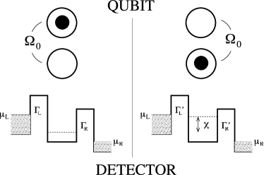
Figure 1: Schematic of a double quantum dot (DQD) qubit and coupled SET. A single excess electron is shared by the DQDs. When the near (far) QD is occupied, the electron tunneling rates through the SET junctions $j={\rm L,R}$ are denoted $\Gamma^{\prime}_{j}$ ($\Gamma_{j}$). The charging energy of the SET island is increased by $\chi$ ($\hbar=1$) when the near QD is occupied.

The SET source and drain leads (reservoirs) are biased to Fermi levels $\mu_{\rm L}$ and $\mu_{\rm R}$, respectively. Associated with each of the qubit states is a tunneling process onto, and a tunneling process off, the SET island. These processes occur at rates denoted $\Gamma_{\rm L}$, $\Gamma^{\prime}_{\rm L}$ (source to island) and $\Gamma_{\rm R}$, $\Gamma^{\prime}_{\rm R}$ (island to drain). A dash indicates that the qubit electron is localized in the nearby QD, which we refer to as the “target”.Wiseman et al. (2001) The average current through the SET is $I^{\prime}=e\Gamma^{\prime}_{\rm L}\Gamma^{\prime}_{\rm R}/\left({\Gamma^{\prime}_{\rm L}+\Gamma^{\prime}_{\rm R}}\right)$ when the target dot is occupied, and $I=e\Gamma_{\rm L}\Gamma_{\rm R}/\left({\Gamma_{\rm L}+\Gamma_{\rm R}}\right)$ when the target dot is unoccupied. For later convenience, we now define the averages $\bar{\Gamma}_{\rm L,R}\equiv\left({\Gamma^{\prime}_{\rm L,R}+\Gamma_{\rm L,R}}\right)/2$ and differences $\Delta\Gamma_{\rm L,R}\equiv\Gamma^{\prime}_{\rm L,R}-\Gamma_{\rm L,R}$.

The Hamiltonian for a charge qubit with energy asymmetry $\varepsilon$ and tunnel-coupling strength $\Omega_{0}$ (see Fig. 1) is $\hat{H}_{\rm qb}=\left({\varepsilon\hat{\sigma}_{z}+\Omega_{0}\hat{\sigma}_{x}}\right)/2$, where $\hat{\sigma}_{x,z}$ are Pauli matrices. We choose units such that $\hbar=1$. For $\varepsilon=0$, and in the absence of measurement, the qubit electron tunnels between the DQDs coherently (that is, existing in superpositions of the two localized states within the dots). For characterizing the measurement quality in Sec. IV it is simpler (and commonplaceShnirman and Schön (1998); Makhlin et al. (2000, 2001, 2002)) to consider the limit of $\Omega_{0}\rightarrow 0$, which we do. However, our master equations (both conditional and unconditional) are valid for non-zero $\Omega_{0}$. When both the SET island and target dot are occupied, the system energy increases by the mutual charging energy, $\chi$. This is described by the coupling Hamiltonian $\hat{H}_{\chi}=\chi\hat{\aleph}\otimes\hat{n}$, where $\hat{\aleph}=\hat{b}^{\dagger}\hat{b}$ and $\hat{n}\equiv(\hat{\sigma}_{z}+\hat{1})/2$ are the respective occupation number operators of the SET island and target dot. For simplicity we do not show the standard Hamiltonians for the source and drain leads, since we trace the leads out of the total state matrix in order to consider only the SET and qubit in the Born-Markov approximation. The Hamiltonian for the SET-DQD system (in the charge basis) is

$$\hat{H}=\hat{1}\otimes\hat{H}_{\rm qb}+\hat{H}_{\chi}\ ,$$ (2)

where $\hat{1}$ is the $2\times 2$ identity matrix. It is simple to diagonalize the qubit Hamiltonian to find the computational/logical basis.Shnirman and Schön (1998) However, we are interested in the measurement process which, for the purposes of this paper, is performed in the charge basis.

III Previous work

In this section we discuss previous work on the continuous monitoring of a charge qubit by a SET. We demonstrate that the master equation of Ref. Shnirman and Schön, 1998 (and those of Refs. Makhlin et al., 2000 and Makhlin et al., 2001, 2002; Goan, 2004 since they are equivalent) can produce non-physical results and therefore is not of the Lindblad form. This master equation was derived independent of the coupling strength $\chi$, but the SET quality analysis always assumed weak coupling. First, we clarify the weak-response and weak-coupling assumptions.

Qualitatively, a weakly responding detector is one in which the variation in the detector’s output that depends on the qubit state is small compared to the average part. KorotkovKorotkov (1999, 2001, 2003) expresses this quantitatively in terms of the current output as

$$\left|{\Delta I}\right|\ll\bar{I},$$ (3)

where $\Delta I\equiv I-I^{\prime}$ and $\bar{I}\equiv\left({I^{\prime}+I}\right)/2$. Note that $\left|{\Delta I}\right|\leq 2\bar{I}$, so that strong response is $\left|{\Delta I}\right|\approx 2\bar{I}$.

The strength of the SET-qubit coupling is quantified by $\chi$ (see Sec. II). When analyzing the quality of the SET, the authors of Refs. Shnirman and Schön, 1998, Makhlin et al., 2000, Makhlin et al., 2001 and Makhlin et al., 2002 make the weak coupling assumption

$$\chi\ll\bar{\Gamma}_{\rm L}+\bar{\Gamma}_{\rm R}.$$ (4)

In Ref. Makhlin et al., 2001 this assumption was made “for definiteness”. It leads to a major simplification in that the SET island charge fluctuation spectrum is ‘white’ over all frequencies of interest. The variations in the SET tunneling rates are proportional to $\chi$,Shnirman and Schön (1998); Makhlin et al. (2000); Korotkov (2001); Makhlin et al. (2001, 2002) so that weak coupling implies weak response. However, a strongly coupled detector can have strong or weak response.

III.1 Unconditional master equation

The unconditional (or nonselective, or ensemble average) master equation of LABEL:SSPRB98 is obtained by averaging over, or ignoring, the measurement record (the number of electrons that have tunneled into the SET drain). This is achieved by setting $k=0$ in equations (20)–(27) of that paper. To perform a quantitative analysis of these equations, it is imagined that the Josephson coupling energy can be “turned off” during the measurement (the equivalent Hamiltonian parameter from Sec. II is $\Omega_{0}$). Using our notations for clarity, the resulting unconditional master equation [equations (31) and (35) of that paper] can be written as

$$\dot{\rho}^{0}_{11} = -\Gamma^{\prime}_{\rm L}\rho^{0}_{11}+\Gamma^{\prime}_{\rm R}\rho^{1}_{11}\ ,$$ (5a)

$$\dot{\rho}^{0}_{22} = -\Gamma_{\rm L}\rho^{0}_{22}+\Gamma_{\rm R}\rho^{1}_{22}\ ,$$ (5b)

$$\dot{\rho}^{0}_{12} = i\varepsilon\rho^{0}_{12}-\bar{\Gamma}_{\rm L}\rho^{0}_{12}+\bar{\Gamma}_{\rm R}\rho^{1}_{12}\ ,$$ (5c)

$$\dot{\rho}^{1}_{11} = \Gamma^{\prime}_{\rm L}\rho^{0}_{11}-\Gamma^{\prime}_{\rm R}\rho^{1}_{11}\ ,$$ (6a)

$$\dot{\rho}^{1}_{22} = \Gamma_{\rm L}\rho^{0}_{22}-\Gamma_{\rm R}\rho^{1}_{22}\ ,$$ (6b)

$$\dot{\rho}^{1}_{12} = i\left({\varepsilon+\chi}\right)\rho^{1}_{12}-\bar{\Gamma}_{\rm R}\rho^{1}_{12}+\bar{\Gamma}_{\rm L}\rho^{0}_{12}\ .$$ (6c)

Here $\rho_{\rm i,j}^{\aleph}$ is the element in the $i$th row and $j$th column of the qubit state matrix conditioned by the SET state $\aleph=0,1$ (the occupation number of the relevant SET island level). The states are normalized so that $P^{\aleph}\equiv\mathrm{Tr}\left[{{\rho^{\aleph}}}\right]$ is the probability that the SET state is $\aleph$. Thus the average qubit state is $\rho^{0}+\rho^{1}$.

We now demonstrate that Eqs. (5) and (6) can produce a non-positive, and therefore non-physical, qubit state matrix. We begin by noting that the following inequality is satisfied by all positive $2\times 2$ matrices.

$$\rho^{\phantom{0}}_{11}\rho^{\phantom{0}}_{22}\geq\left|{\rho^{\phantom{0}}_{12}}\right|^{2}\ .$$ (7)

Now consider the short-time solution for $\rho^{0}$ [Eqs. (5)] when the SET is initially occupied ($\rho^{0}=0$ at $t=0$) and the qubit is in the following superposition state: $\rho^{1}_{11}=\rho^{1}_{22}=\rho^{1}_{12}=\frac{1}{2}$. After an infinitesimally short time $\delta t$, we have

$$\rho^{0}_{11} \approx \mbox{$\frac{1}{2}$}\Gamma^{\prime}_{\rm R}\delta t\ ,$$

$$\rho^{0}_{22} \approx \mbox{$\frac{1}{2}$}\Gamma_{\rm R}\delta t\ ,$$ (8)

$$\rho^{0}_{12} \approx \mbox{$\frac{1}{2}$}\bar{\Gamma}_{\rm R}\delta t\ .$$

Substituting these into Eq. (7), canceling factors of $\left({\delta t}\right)^{2}/4$ on both sides, and rearranging gives

$$\left|{\Delta\Gamma_{\rm R}}\right|^{2}\leq 0\ ,$$ (9)

which is false for all values of $\Gamma^{\prime}_{\rm R}\neq\Gamma_{\rm R}$. The case of $\Gamma^{\prime}_{\rm R}=\Gamma_{\rm R}$ corresponds to there being no response from the SET for a change in the qubit state, i.e. no measurement is being performed. The result (9) shows that the inequality (7) is not satisfied, positivity is not preserved, and the master equation of LABEL:SSPRB98 is not of the Lindblad form. This is also true of the equivalent master equations presented in Refs. Makhlin et al., 2000, Makhlin et al., 2001, Makhlin et al., 2002 and Goan, 2004. Numerical results show that the violation of Eq. (7) occurs only for short times (compared to the characteristic qubit decoherence and measurement times). However, since the qubit state matrix for later times is determined by the (non-positive) state matrix for short times, one cannot be confident in the ability of the state matrix at later times to describe a real physical system. Therefore, we maintain that the master equations of Refs. Shnirman and Schön, 1998, Makhlin et al., 2000, Makhlin et al., 2001, Makhlin et al., 2002 and Goan, 2004 cannot be relied upon at any time.

IV Quantifying the Sensitivity and Back-action

In the previous section we showed that previous master equations for the SET-monitored charge qubit are not of the Lindblad form. In Sec. V we derive a Lindblad-form master equation (and “unravel”Carmichael (1993) it into a conditional master equation), which requires strong coupling between the SET and the qubit. In the strong coupling régime it is natural for the detector also to be strongly responding since, as mentioned, the coupling energy largely determines the detector’s response. The more traditional measures of sensitivity and back-action in this type of measurement areShnirman and Schön (1998); Makhlin et al. (2000); Korotkov (2001); Makhlin et al. (2001, 2002) the measurement time $\tau_{\rm m}$ and decoherence rate $\Gamma_{\rm d}$, respectively. Previous definitions of these quantities assumed weak detector response, either explicitly or implicitly. Therefore it is necessary to use more general definitions, which we give in this section.

IV.1 Decoherence Time

Previously the decoherence rate $\Gamma_{\rm d}$ was defined as the rate at which the coherences in the qubit decay according to the unconditional master equation. For charge qubit measurements by a QPC, this description is unambiguous: there is one decay rate for the coherences which can be obtainedGurvitz (1997) by inspection of the master equation. This is not the case for the SET because there are two qubit state matrices, namely $\rho^{0}$ and $\rho^{1}$, conditioned by the SET island state. Our master equation (19) gives a rate of decay for each of these conditional qubit coherences, neither of which alone accurately represents the average decoherence of the qubit state $\rho=\rho^{0}+\rho^{1}$. In Refs. Shnirman and Schön, 1998, Makhlin et al., 2000, Makhlin et al., 2001, and Makhlin et al., 2002, the qubit decoherence rate is defined as the slowest of these two rates under the premise that the qubit state cannot collapse any faster. This therefore represents an over-estimate of the quality of the measurement device, as it minimizes Eq. (1).

In an effort to more precisely quantify the decoherence, we find a characteristic qubit decoherence time by borrowing a technique from the field of quantum optics. In a typical quantum optics scenario, where the detector signal consists of absorption of photons emitted by a quantum system, the coherence of the source is defined by the Glauber coherence function.Glauber (1963) For a two-level quantum system (such as the two-level atom) this is given in terms of the steady-state, two-time correlation function $g(\tau)=\left\langle{\hat{\sigma}^{\dagger}(\tau)\hat{\sigma}0}\right\rangle_{\rm ss}$. Here $\hat{\sigma}=|{0}\rangle\langle{1}|$ is the lowering operator for the atom (in the Heisenberg picture). The expression involves the lowering operator because the detection involves absorption.

In the solid-state context where the detection does not “lower” the DQD state it is more appropriate to consider an expression that treats $|{0}\rangle$ and $|{1}\rangle$ symmetrically. The obvious expression is

$$g(\tau)\equiv\left\langle{\hat{\sigma}^{\dagger}(\tau)\hat{\sigma}0}\right\rangle_{\rm ss}+\left\langle{\hat{\sigma}(\tau)\hat{\sigma}^{\dagger}0}\right\rangle_{\rm ss}^{*}\ .$$ (10)

In the Schrödinger picture, this coherence function can be expressed as

$$g(\tau) = \mathrm{Tr}\left[{{\hat{\sigma}^{\dagger}{\rho}^{-}(\tau)}}\right]+\mathrm{Tr}\left[{{\hat{\sigma}{\rho}^{+}(\tau)}}\right]^{*}$$ (11)

$$\equiv {\rho}^{-}_{21}(\tau)+\left[{{\rho}^{+}_{12}(\tau)}\right]^{*}\ ,$$

where ${\rho}(\tau)=\exp\left({\mathcal{L}_{\rho}\tau}\right){\rho}(0)$, ${\rho}^{+}(0)\equiv\hat{\sigma}^{\dagger}\rho_{\rm ss}$, and ${\rho}^{-}(0)\equiv\hat{\sigma}\rho_{\rm ss}$. The Liouvillian $\mathcal{L}_{\rho}$ is the qubit time evolution superoperator [analogous to $\mathcal{L}$ in Eq. (19)].

The coherence function thus defined has the property that it is normalized in the sense that $g(0)\equiv 1$ and $\lim_{\tau\to\infty}g(\tau)=0$. Therefore we can now define the decoherence time (which means the same as the coherence time) asGardiner and Zoller (2000)

$$\tau_{\rm d}\equiv\int_{0}^{\infty}g(\tau)d\tau.$$ (12)

The decoherence rate is simply $\Gamma_{\rm d}=\tau_{\rm d}^{-1}$. For an exponentially decaying coherence it is easy to verify that $\Gamma_{\rm d}$ is the exponential decay coefficient. For example, for the QPC master equation of LABEL:GoaMilWisSunPRB01, this coherence function technique yields the same decoherence rate as the QPC models of Refs. Korotkov, 1999, Gurvitz, 1997 and Goan et al., 2001 (see Appendix A).

IV.2 Measurement Time

PreviouslyShnirman and Schön (1998); Makhlin et al. (2000, 2001, 2002) the measurement time $\tau_{\rm m}$ was defined as follows. Keeping track of the number of electrons $N_{\rm R}(t)$ that have tunneled into the drain during the measurement process (while ignoring the information contained by electrons tunneling from the source onto the island) allows tracking of the dynamics of the probability distribution for this number, $P(N_{\rm R},t)$. Gaussian statistics were assumed for $N_{\rm R}$, thereby implicitly assuming weak detector response (many SET tunneling events occur before the qubit states are distinguishable). After starting the measurement as a delta function at $N_{\rm R}=0$, $P(N_{\rm R},t)$ displays two peaks (corresponding to the two qubit states) which drift linearly in time to positive values of $N_{\rm R}$ with velocities $\Gamma\equiv I/e$ and $\Gamma^{\prime}\equiv I^{\prime}/e$, respectively. The widths of the peaks broaden due to counting statistics, growing as $\sqrt{f\Gamma t}$ and $\sqrt{f^{\prime}\Gamma^{\prime}t}$, respectively.Makhlin et al. (2002) In Refs. Makhlin et al., 2000 and Makhlin et al., 2001 these are given with an extra factor of $\sqrt{2}$ as $\sqrt{2f\Gamma t}$ and $\sqrt{2f^{\prime}\Gamma^{\prime}t}$. Here the Fano factors are $f=\left({{\Gamma}_{\rm L}^{2}+{\Gamma}_{\rm R}^{2}}\right)/\left({{\Gamma}_{\rm L}+{\Gamma}_{\rm R}}\right)^{2}$ and $f^{\prime}=\left({{\Gamma}_{\rm L}^{\prime 2}+{\Gamma}_{\rm R}^{\prime 2}}\right)/\left({{\Gamma}^{\prime}_{\rm L}+{\Gamma}^{\prime}_{\rm R}}\right)^{2}$. The peaks emerge from the broadened distribution when the separation of the distributions is larger than their widths, $\left|{\Gamma-\Gamma^{\prime}}\right|t\geq\left({\sqrt{f\Gamma t}+\sqrt{f^{\prime}\Gamma^{\prime}t}}\right)$.

Fundamentally, the measurement time relates to distinguishing the qubit states using information gained from the detector. This obviously involves the conditioned state of the qubit. Since the quantum trajectory equation is by definition the optimal way to process the detector current to get information about the qubit, it should be used to define the measurement time. Our quantum trajectory equation is given in Sec. V.

In the measurement basis we can, quite generally, define an uncertainty function for the qubit state as the conditional variance in $\hat{\sigma}_{z}$:

$$V(t) = {\rm E}\left[{\left\langle{\hat{\sigma}_{z}^{2}}\right\rangle_{\rm c}(t)-\left\langle{\hat{\sigma}_{z}}\right\rangle_{\rm c}^{2}(t)}\right]$$ (13a)

$$= 1-{\rm E}\left[{z_{\rm c}^{2}(t)}\right].$$ (13b)

Here the subscript c denotes conditional variables, E[ $\cdot$ ] denotes a classical expectation value, and $\left\langle{\cdot}\right\rangle$ denotes a quantum average (we use $z$ as shorthand for $\left\langle{\hat{\sigma}_{z}}\right\rangle$). The initial state is the unconditional steady state, that is, the long-time limit of the master equation given in Sec. V.

Provided that the qubit Hamiltonian commutes with the measured observable, i.e. $\hat{\sigma}_{z}$, the measurement will not disturb the qubit populations (but will necessarily affect the qubit coherence). Thus, for a non-disturbing measurement we require $\Omega_{0}=0$. In this case, $V(t)$ will have the properties that $V(0)=1$, and $\lim_{\tau\to\infty}V(\tau)=0$. That is, we start off with no knowledge of $\hat{\sigma}_{z}$ and end up with complete knowledge. Thus, in analogy with Eq. (12), it can be used to give a general definition of the measurement time as

$$\tau_{\rm m}\equiv\int_{0}^{\infty}V(\tau)d\tau.$$ (14)

However, because $V(t)$ arises from stochastic evolution, it is not generally possible to obtain an analytical expression for $V(\tau)$, unlike $g(\tau)$, which arises from the deterministic evolution of the master equation. If $V(t)$ decays exponentially with time, then $\tau_{\rm m}$ can be evaluated as

$$\tau_{\rm m}^{-1}=-\left.\frac{dV(t)}{dt}\right|_{t=0}.$$ (15)

This equation (expressed differently) was first used in Ref. Wiseman et al., 2001. It has the advantage that it can be evaluated analytically. (In Appendix A we report this calculation for the QPC.) As we will see later, for the SET in a wide range of parameter régimes, the exponential approximation for $V(\tau)$ is a good one, so that Eq. (15) can be used.

V Strongly coupled SET

Using the quantum trajectory approach developed in quantum optics,Carmichael (1993) we describe both the conditionalKorotkov (1999); Wiseman et al. (2001) and better-known unconditionalGurvitz (1997) time evolution of the charge qubit state whilst undergoing continuous measurement by a SET. In order to consider the tunneling processes through the SET as distinguishable, that is, in order to ignore the finite widths $\Gamma_{\rm L,R}$ and $\Gamma^{\prime}_{\rm L,R}$ of these tunneling processes, requiresBeenakker (1991)

$$\chi\gg\bar{\Gamma}_{\rm L}+\bar{\Gamma}_{\rm R}\ .$$ (16)

This assumption of a strongly coupled SET is critical to our ability to derive a master equation using our approach. As mentioned in Sec. II, the qubit energy asymmetry is shifted by $\chi$ when both the SET island and the target dot are occupied. For the strongly coupled SET, this causes a large shift ($\propto\chi$) in the qubit Rabi frequency ($\Omega=\sqrt{\Omega_{0}^{2}+\varepsilon^{2}}$). One could conceivably posit that this situation cannot be considered as measurement as it has such a large effect on the qubit state. However, because this energy shift is in the same basis as the measurement, it affects only the qubit coherence and not the populations. We analyze this below.

Note that the time to determine the qubit state (the measurement time) is related to the time it takes to distinguish between the two corresponding currents through the SET. Intuitively, larger separation between these two currents decreases the measurement time. Indeed, this leads to the prediction that the strongly responding SET would enable faster charge qubit measurement than its weakly responding counterpart. Qualitatively, the largest separation of these currents occurs when tunneling through the SET switches between on and off for the two qubit states. When the SET is operated near this so-called “switching point”, thermal fluctuations and higher-order processes such as cotunneling become the leading contribution to the current.Shnirman and Schön (1998) As these processes yield very small currents,Schoelkopf et al. (2003) they may well be negligible in a laboratory setting. Nevertheless, we assume that the SET conducts for both qubit states to ensure that higher-order processes are negligible. Figure 2 shows this assumption schematically on a hypothetical SET conductance-oscillation plot. The qubit state shifts the gate voltage by an amount that changes the SET conductance significantly for the case of strong response, while remaining always in a conducting state.

We represent the combined state of the SET island and qubit by the composite state matrix

$$G(t)=|{0}\rangle\langle{0}|_{\rm SET}\otimes\rho^{0}(t)+|{1}\rangle\langle{1}|_{\rm SET}\otimes\rho^{1}(t)\ ,$$ (17)

where $\rho(t)=\mathrm{Tr}\left[{{G(t)}}\right]=\rho^{0}(t)+\rho^{1}(t)$ is the qubit state matrix, the superscript again referring to the SET island occupation ($\aleph=0$ or $1$). We reiterate that, although we consider the state of the SET island in a composite density matrix with the qubit, no charge superposition states exist on the SET island. We present master equations for $G(t)$ for compactness, but could equally well present coupled master equations for the qubit states $\rho^{0}(t)$ and $\rho^{1}(t)$ as in Refs. Makhlin et al., 2000 and Makhlin et al., 2001, 2002; Goan, 2004, for example.

Figure 2: Hypothetical SET conductance vs SET gate voltage. The two dots show the SET conductance corresponding to the two qubit eigenstates for the case of strong response.

V.1 Unconditional master equation

Here we present our unconditional master equation for the state matrix $G(t)$ of the system (qubit plus SET island). We will first outline the details of its derivation, which closely follows the derivation in the appendix of LABEL:WisetalPRB01. We first consider the state matrix $W(t)$ for the combined system (qubit, SET and leads). The leads are treated as perfect Fermi thermal reservoirs with very fast relaxation constants. Each lead then remains in thermal equilibrium at its respective chemical potential. We define a time interval $\Delta t$ that is long compared to the relaxation time of the leads, but short (infinitesimal) compared to the dynamics of the SET island and qubit. Transforming to an interaction picture with respect to $\hat{H}$ [Eq. (2)] leaves only tunnel-coupling terms (between the leads and the SET island) in the interaction picture Hamiltonian $\hat{H}_{\rm i}$. The change in $W(t)$ from time $t$ to $t+\Delta t$ to second order in the tunnel-coupling energy is then given by

$$W(t+\Delta t) = W(t)-i\Delta t\left[{\hat{H}_{\rm i},W(t)}\right]$$

$$-\Delta t\int_{t}^{t+\Delta t}dt^{\prime}\left[{\hat{H}_{\rm i}(t^{\prime}),\left[{\hat{H}_{\rm i}(t^{\prime}),W(t^{\prime})}\right]}\right].$$

We now make a Markov approximation for the instantaneous relaxation of the source (L) and drain (R) leads so that $W(t)=G(t)\otimes\rho_{\rm L}\otimes\rho_{\rm R}$, and we find the resulting evolution equation for $G(t)$ by tracing over the leads. Assuming that all tunneling occurs from source to drain ($k_{\rm B}T\ll eV$) and moving back to the Schrödinger picture, we obtain the unconditional master equation for $G(t)$ as

$$\dot{G} = -i\left[{\hat{H},G}\right]+\Gamma^{\prime}_{\rm L}{\cal D}\left[{{\hat{b}^{\dagger}\otimes\hat{n}}}\right]G+\Gamma^{\prime}_{\rm R}{\cal D}\left[{{\hat{b}\otimes\hat{n}}}\right]G$$ (19)

$$+\Gamma_{\rm L}{\cal D}\left[{{\hat{b}^{\dagger}\otimes(\hat{1}-\hat{n})}}\right]G+\Gamma_{\rm R}{\cal D}\left[{{\hat{b}\otimes(\hat{1}-\hat{n})}}\right]G$$

$$\equiv {\cal L}G,$$

which is explicitly of the Lindblad form, and we have omitted time arguments of $G$ for brevity. We remind the reader that $\hat{b}=|{0}\rangle\langle{1}|_{\rm SET}$, $\hat{n}=\left({\hat{\sigma}_{z}+1}\right)/2$ is the target dot occupation operator, and $\hat{H}$ is given by Eq. (2). In deriving Eq. (19), our assumption of strong SET-qubit coupling ($\chi\gg\bar{\Gamma}_{\rm L}+\bar{\Gamma}_{\rm R}$) is the main difference between our assumptions and those of the previous models.Shnirman and Schön (1998); Makhlin et al. (2000, 2001, 2002); Goan (2004) This assumption is essential to our ability to derive our master equation, as it allows each lead to be treated as two independent baths that differ in energy by $\hbar\chi$. The Lindblad superoperator ${\cal D}$ in Eq. (19) represents the dissipative, irreversible part of the qubit evolution — the measurement-induced decoherence. It is defined asWiseman and Milburn (1993)

$${\cal D}\left[{{\hat{x}}}\right]G\equiv{\cal J}\left[{{\hat{x}}}\right]G-{\cal A}\left[{{\hat{x}}}\right]G\ ,$$ (20)

where ${\cal J}\left[{{\hat{x}}}\right]G\equiv\hat{x}G\hat{x}^{\dagger}$, and ${\cal A}\left[{{\hat{x}}}\right]G\equiv\mbox{$\frac{1}{2}$}\left({\hat{x}^{\dagger}\hat{x}G+G\hat{x}^{\dagger}\hat{x}}\right)$. GoanGoan (2004) expressed the master equation of Eqs. (5)–(6) in a similar form to Eq. (19). The crucial differences, i.e. the non-Lindblad terms in Eqs. (5)–(6), are shown in Appendix B.

The unconditional master equation (19) describes the system evolution when the measurement result is ignored or averaged over. When quantifying the SET measurement quality, we assume a non-disturbing measurement as noted in the paragraph preceding Eq. (14). That is, we assume $\Omega_{0}=0$ (as was assumed in previous quantitative analysesShnirman and Schön (1998); Makhlin et al. (2000, 2001, 2002) of the SET measurement quality). In order for our master equation to have a unique steady-state solution, we require nonzero $\Omega_{0}$. Thus, for numerical simulations we use $\Omega_{0}=0.01\Gamma_{\rm L}$. Note however, that Eq. (19) is valid for any $\Omega_{0}\ll\chi$. The numerical solution of the master equation (19) gives oscillating, decaying off-diagonal elements of the qubit state matrix. We quantify this by the coherence function $g(\tau)$ given in Eq. (11). For SET monitoring of the qubit, ${\cal L}$ acts on the qubit-plus-SET state $G$, so $\rho$ must be replaced by $G$ in the coherence function of Eq. (11). The resulting $g(\tau)$ is shown in Fig. 3.

The four subplots in Fig. 3 correspond to increasing values of SET response $\left|{\Delta I}\right|/\bar{I}$, which is bounded above by $2$. The strength of the SET response was modified by varying $\Gamma^{\prime}_{\rm L}$ — the slowest rate of tunneling onto the SET island. The initial qubit state is completely mixed:

$$\rho_{\rm ss}=\frac{1}{2}\hat{1},$$ (21)

and the SET island is initially in the corresponding steady-state, which is represented by the island occupation probability $P^{1}=\mathrm{Tr}\left[{{\rho^{1}}}\right]$ (with $P^{0}=1-P^{1}$) as

$$P^{1}_{\rm ss}=\frac{\bar{\Gamma}_{\rm L}}{\bar{\Gamma}_{\rm L}+\bar{\Gamma}_{\rm R}}.$$ (22)

The strongest SET response [in Fig. 3 (d)] corresponds to

$$0<\Gamma^{\prime}_{\rm L}\ll\Gamma_{\rm L}\sim\Gamma_{\rm R}\sim\Gamma^{\prime}_{\rm R},$$ (23)

where we assume that $\Gamma_{\rm L}^{\prime}$ is large enough in order to ignore higher-order processes such as cotunneling.

The rapid oscillations in Fig. 3 are due to the strong SET-qubit coupling given in Eq. (16). Thus, these oscillations are very fast compared to the tunneling rates. As a consequence, even if an individual tunneling event could be detected, it would be impossible to know when it occurred with sufficient accuracy to allow the phase of the oscillation to be known. This is a direct result of the strong coupling assumption (16) required for our Lindblad-form master equation. In the observable qubit state, the rapid oscillations are effectively averaged over. This produces the observable decoherence given by the bold line in Fig. 3.

The observable state can be obtained from $G(t)$ by moving to an interaction picture with respect to $\hat{H}_{\chi}$, unique from the interaction picture mentioned in the derivation of Eq. (19), and making a rotating wave approximation by dropping all rapidly oscillating terms (those involving $\chi$). The result is the following master equation

$$\dot{\widetilde{G}} = -i\left[{\widetilde{H}_{\rm I},\widetilde{G}}\right]+\Gamma^{\prime}_{\rm L}{\cal D}\left[{{\hat{b}^{\dagger}\otimes\hat{n}}}\right]\widetilde{G}+\Gamma^{\prime}_{\rm R}{\cal D}\left[{{\hat{b}\otimes\hat{n}}}\right]\widetilde{G}$$ (24)

$$+\Gamma_{\rm L}{\cal D}\left[{{\hat{b}^{\dagger}\otimes(\hat{1}-\hat{n})}}\right]\widetilde{G}+\Gamma_{\rm R}{\cal D}\left[{{\hat{b}\otimes(\hat{1}-\hat{n})}}\right]\widetilde{G}$$

$$\equiv \widetilde{\mathcal{L}}\widetilde{G},$$

where the observable state $\widetilde{G}$ is given by

$$\widetilde{G}=|{0}\rangle\langle{0}|_{\rm SET}\otimes\tilde{\rho}^{0}+|{1}\rangle\langle{1}|_{\rm SET}\otimes\tilde{\rho}^{1},$$ (25)

with $\tilde{\rho}^{0}\equiv\rho^{0}$ and $\tilde{\rho}^{1}\equiv\mathrm{diag}\left({\rho^{1}_{11},\rho^{1}_{22}}\right)$. The Hamiltonian in this interaction picture (after the rotating wave approximation) is

$$\widetilde{H}_{\rm I}=|{0}\rangle\langle{0}|_{\rm SET}\otimes\hat{H}_{\rm qb}+|{1}\rangle\langle{1}|_{\rm SET}\otimes\frac{\varepsilon}{2}\hat{\sigma}_{z}.$$ (26)

Thus we see that in the interaction picture (which reflects the observable effects of the actual dynamics), no qubit coherence exists when the SET is occupied. That is, the off-diagonal elements of ${\rho}^{1}$ are equal to zero.

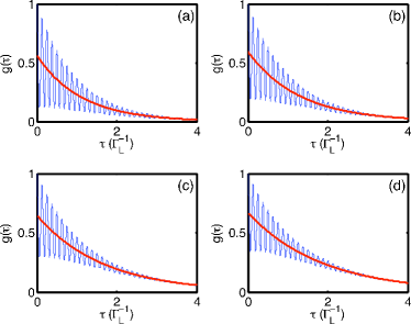
Figure 3: Decoherence of a charge qubit undergoing continuous measurement by a strongly responding SET. The rapid oscillations are too fast to be observable — the thick line shows the observable result. From (a) to (d): $\left|{\Delta I}\right|/\bar{I}=1/10$, $1/3$, $1$, and $3/2$. Other parameters were $\Omega_{0}=0.01\Gamma_{\rm L}$, $\chi=50\Gamma_{\rm L}$, $\Gamma_{\rm R}=1.1\Gamma_{\rm L}$, $\Gamma^{\prime}_{\rm R}=1.2\Gamma_{\rm L}$.

Using the observable state (25) we obtain the following analytical expression for the observable coherence function

$$g_{\rm obs}(\tau)=P^{0}_{\rm ss}\exp\left({-\bar{\Gamma}_{\rm L}\tau}\right),$$ (27)

which gives the qubit decoherence time of

$$\tau_{\rm d} \equiv \int_{0}^{\infty}g_{\rm obs}(\tau)d\tau$$ (28)

$$= \frac{P^{0}_{\rm ss}}{\bar{\Gamma}_{\rm L}}=\frac{\bar{\Gamma}_{\rm R}}{\bar{\Gamma}_{\rm L}\left({\bar{\Gamma}_{\rm L}+\bar{\Gamma}_{\rm R}}\right)}.$$

The result (27) is plotted in Fig. 3 as a bold line. This indicates that our requirement for $\chi\gg\bar{\Gamma}_{\rm L}+\bar{\Gamma}_{\rm R}$ results in an effectively immediate loss of a portion [$\bar{\Gamma}_{\rm R}/(\bar{\Gamma}_{\rm L}+\bar{\Gamma}_{\rm R})$] of the qubit coherence upon commencing measurement, followed by exponential decay at the rate $\bar{\Gamma}_{\rm L}$.

It is interesting to note that in the unlikely event of the SET island state being known to be occupied at the start of the measurement (so that $P^{0}=0$), the qubit is observed to completely decohere instantaneously. This fact alone shows that the quality of charge qubit measurements by a SET cannot be captured by a simple quantity such as $\Gamma_{\rm d}\tau_{\rm m}$, although this can provide some insight into the measurement quality. Note also that $g_{\rm obs}(\tau)$ depends minimally on the SET response.

V.2 Conditional master equation

We obtain the conditional (or selective, or stochastic) evolution of $G(t)$, denoted by a subscript c, in a similar way as in Ref. Wiseman et al., 2001. However, we do not eliminate the SET island state as in LABEL:WisetalPRB01, which was achieved by setting $\Gamma^{\prime}_{\rm R},\Gamma_{\rm R}\gg\Gamma^{\prime}_{\rm L},\Gamma_{\rm L}$. Our result is the following Itō Gardiner (1985) conditional master equation (quantum trajectory/filtering equation), where the SET-qubit state is conditioned on the tunneling events both on and off the SET island:

$$dG_{\rm c} = \sum_{j=\rm L,R}dN_{j}\left\{{\frac{{\cal S}_{j}}{\mathrm{Tr}\left[{{{\cal S}_{j}G_{\rm c}}}\right]}-1}\right\}G_{\rm c}$$ (29)

$$-dt~{}\!{\cal H}\left[{{\mbox{$\frac{1}{2}$}\hat{\Upsilon}+i\hat{H}}}\right]G_{\rm c}\ ,$$

where the non-linear superoperator $\mathcal{H}$ is defined by ${\cal H}\left[{{\hat{x}}}\right]G\equiv\hat{x}G+G\hat{x}^{\dagger}-\mathrm{Tr}\left[{{\left({\hat{x}+\hat{x}^{\dagger}}\right)G}}\right]G$. The operator $\hat{\Upsilon}$ and superoperators ${\cal S}_{\rm L}$ and ${\cal S}_{\rm R}$ are given by

$$\hat{\Upsilon} \equiv \Gamma^{\prime}_{\rm L}\hat{b}\hat{b}^{\dagger}\otimes\hat{n}+\Gamma_{\rm L}\hat{b}\hat{b}^{\dagger}\otimes(\hat{1}-\hat{n})$$ (30a)

$$~{}+~{}\Gamma^{\prime}_{\rm R}\hat{b}^{\dagger}\hat{b}\otimes\hat{n}+\Gamma_{\rm R}\hat{b}^{\dagger}\hat{b}\otimes(\hat{1}-\hat{n})\ ,$$

$${\cal S}_{\rm L} \equiv \Gamma^{\prime}_{\rm L}{\cal J}\left[{{\hat{b}^{\dagger}\otimes\hat{n}}}\right]+\Gamma_{\rm L}{\cal J}\left[{{\hat{b}^{\dagger}\otimes(\hat{1}-\hat{n})}}\right]\ ,$$ (30b)

$${\cal S}_{\rm R} \equiv \Gamma^{\prime}_{\rm R}{\cal J}\left[{{\hat{b}\otimes\hat{n}}}\right]+\Gamma_{\rm R}{\cal J}\left[{{\hat{b}\otimes(\hat{1}-\hat{n})}}\right]\ .$$ (30c)

In Eq. (29) we have introduced the classical random point processes $dN_{\rm L}(t)$ and $dN_{\rm R}(t)$. They represent the number (either 0 or 1) of electron tunneling events from source to island (L) and island to drain (R), respectively, in an infinitesimal time interval $[t,t+dt)$. In the sequential tunneling mode, at most one of these may be nonzero for each particular infinitesimal interval of time. That is, an electron cannot tunnel through the entire SET ‘in one go’, so to speak. The conditional master equation for the observable state (25) is identical to (29), but with $\widetilde{G}$ in place of $G$ and $\widetilde{H}_{\rm I}$ in place of $\hat{H}$.

The two terms summed in the first line of Eq. (29) represent electron tunneling events onto (L) and off (R) the SET island. Each event is represented by an incoherent mixture of the two possible paths by which this can occur (corresponding to the two localized electron states within the qubit). The final line in Eq. (29) represents the evolution of $G_{\rm c}(t)$ that is due to the Hamiltonian and the null measurement of no SET tunneling events in the time interval $[t,t+dt)$. It is important to note that these microscopic processes may not necessarily be directly observed by a realistic observer.Oxtoby et al. (2003, 2005) Nevertheless, it is sensible to unravel the master equation (19) into a quantum jumpWiseman and Milburn (1993) stochastic master equation because the underlying physical process consists of single electron tunneling events.

The ensemble-average evolution of $G(t)$ [Eq. (19)] can be recovered by averaging over all possible trajectories given by Eq. (29). In the Itō formalism,Gardiner (1985) this simply involves replacing the stochastic increments $dN_{\rm L}$ and $dN_{\rm R}$ in Eq. (29) with their expectation values, which can self-consistently be given in terms of their respective quantum averages:

$$\mathrm{E}\left[{dN_{\rm L,R}(t)}\right]={dt~{}\!}\mathrm{Tr}\left[{{{\cal S}_{\rm L,R}G_{\rm c}(t)}}\right].$$ (31)

Having presented the quantum trajectory equation (29), we are now in a position to consider the SET measurement sensitivity using $\tau_{\rm m}$ and $V(t)$ defined in Sec. IV.2. We proceed by noting that the qubit state matrix $\rho$ can be represented in terms of the Pauli spin matrices as

$$\rho^{\aleph}=\mbox{$\frac{1}{2}$}\left({P^{\aleph}\hat{1}+x^{\aleph}\hat{\sigma}_{x}+y^{\aleph}\hat{\sigma}_{y}+z^{\aleph}\hat{\sigma}_{z}}\right)\ .$$ (32)

The conditional master equation [for the observable state (25)] can be expressed in terms of the conditional Bloch sphere variables $x^{\aleph}_{\rm c}$, $y^{\aleph}_{\rm c}$, and $z^{\aleph}_{\rm c}$, as well as the conditional SET island occupation probabilities $P^{\aleph}_{\rm c}$. The conditioning here is upon both the measurement results (subscript c) and the SET island state (superscript 0 or 1). To find $V(t)$ (and hence approximate $\tau_{\rm m}$), we are interested in the expectation value of $(z_{\rm c})^{2}=(z^{0}_{\rm c}+z^{1}_{\rm c})^{2}$. Averaging over the jumps in the conditional master equation for $z_{\rm c}$ and using the fact that stochastic variables satisfy $d(z^{2})=2zdz+dzdz$, we obtain the following equation for the time rate of change of this expectation value:

$$\frac{d{\rm E}\left[{z_{\rm c}^{2}}\right]}{dt} = \mathrm{E}\left[\frac{\left({2\bar{\Gamma}_{\rm L}z_{\rm c}^{0}+P^{0}_{\rm c}\Delta\Gamma_{\rm L}}\right)^{2}}{4P^{0}_{\rm c}\bar{\Gamma}_{\rm L}+2\Delta\Gamma_{\rm L}z_{\rm c}^{0}}\right.$$ (33)

$$\left.\phantom{ee}+\frac{\left({2\bar{\Gamma}_{\rm R}z_{\rm c}^{1}+P^{1}_{\rm c}\Delta\Gamma_{\rm R}}\right)^{2}}{4P^{1}_{\rm c}\bar{\Gamma}_{\rm R}+2\Delta\Gamma_{\rm R}z_{\rm c}^{1}}\right].$$

Knowing this and using Eq. (21) to give $z^{\aleph}_{\rm c}(0)=0$, we find from Eq. (15) that

$$\tau_{\rm m}^{-1} \approx P^{0}_{\rm ss}\frac{\left({\Delta\Gamma_{\rm L}}\right)^{2}}{4\bar{\Gamma}_{\rm L}}+P^{1}_{\rm ss}\frac{\left({\Delta\Gamma_{\rm R}}\right)^{2}}{4\bar{\Gamma}_{\rm R}}$$ (34)

$$= \frac{\bar{\Gamma}_{\rm L}\bar{\Gamma}_{\rm R}}{\bar{\Gamma}_{\rm L}+\bar{\Gamma}_{\rm R}}\left[{\left({\frac{\Delta\Gamma_{\rm L}}{2\bar{\Gamma}_{\rm L}}}\right)^{2}+\left({\frac{\Delta\Gamma_{\rm R}}{2\bar{\Gamma}_{\rm R}}}\right)^{2}}\right].$$

A more precise value for the measurement time is obtained from Eq. (13) by numerical solution of the conditional master equation for the observable state. Figure 4 shows plots of $V(t)=1-{\rm E}\left[{z_{\rm c}^{2}(t)}\right]$ for a strongly coupled SET for the same parameter values as the corresponding plots in Fig. 3. Notice that the analytical approximation (the solid line) agrees very well with all of the numerical results (dashed lines). A comparison of Figs. 3 and 4 shows that the strongly responding SET [in plots (d)] has comparable decoherence and measurement times because the functions $V(t)$ and $g_{\rm obs}(\tau)$ are comparable in magnitude at all times.

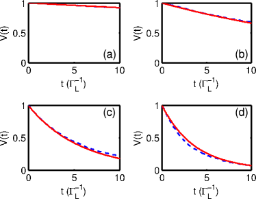
Figure 4: The variance in $\hat{\sigma}_{z}$ (the population difference operator in the measurement basis), $V(t)=1-{\rm E}\left[{z_{\rm c}^{2}(t)}\right]$. The dashed line is an average over 2000 trajectories obtained using the conditional master equation. The solid line is the analytical approximation assuming exponential decay of $V(t)$. Other details are as in Fig. 3.

V.3 Quality Of The Measurement

PreviouslyShnirman and Schön (1998); Makhlin et al. (2000); Korotkov (2001); Makhlin et al. (2001, 2002) the quality of the measurement of a charge qubit by a (weakly responding) SET has been quantified by comparing qubit decoherence and measurement times, with the quantum limit for a weakly responding device given by Eq. (1).

More generally, the purity of the conditioned qubit state (conditioned by measurement results) provides the means to determine the ‘ideality’ of the detector (how close to the quantum limit the detector is operating). This is because an “ideal” detector will preserve a pure qubit state throughout the measurement. Thus, we maintain that the purity of the conditioned qubit state is the ultimate quantifier of measurement quality. The conditioned state of the qubit can only be obtained from the conditional master equation.

In this subsection we analyze the quality of the measurement in two ways. We first use the traditional technique of comparing the qubit decoherence (back-action) and measurement (sensitivity) times using our definitions for these quantities from Sec. IV. We then analyze the average purity of the conditioned qubit state during the measurement.

V.3.1 Comparison: Measurement time and Decoherence Time

Comparing qubit measurement and decoherence time-scales gives an intuitive idea of the quality of the measurement. If these time-scales are of the same order, then we can say that the detector is operating close to the quantum limit. Using Eqs. (28) and (34) we can obtain an analytical approximation for $\Gamma_{\rm d}\tau_{\rm m}$. The result is

$$\Gamma_{\rm d}\tau_{\rm m}\approx\frac{\left({1+\bar{\Gamma}_{\rm L}/\bar{\Gamma}_{\rm R}}\right)^{2}}{\left({\Delta\Gamma_{\rm L}/2\bar{\Gamma}_{\rm L}}\right)^{2}+\left({\Delta\Gamma_{\rm R}/2\bar{\Gamma}_{\rm R}}\right)^{2}}.$$ (35)

This result is a valid approximation when $V(t)$ is a decaying exponential, which is valid for a wide range of parameter values as shown in Fig. 4. The minimum for Eq. (35) is $1/2$, which occurs only for $\bar{\Gamma}_{\rm L}\ll\bar{\Gamma}_{\rm R}$ (high SET asymmetry) and $\Delta\Gamma_{\rm L,R}\approx 2\bar{\Gamma}_{\rm L,R}$.The second condition requires both $\Gamma^{\prime}_{\rm L}\ll\Gamma_{\rm L}$ and $\Gamma_{\rm R}\ll\Gamma^{\prime}_{\rm R}$, which could in theory be realized by careful arrangement of the SET parameters (specifically bias and gate voltages, and tunnel junction conductances).

V.3.2 Average Purity of the Conditioned Qubit State

Averaging the purity of the conditioned qubit state for the four ensembles in Fig. 4 gives the results in Fig. 5. Here we choose the qubit to start in a pure state [a superposition with $z(0)=0$], rather than a mixture. At the commencement of the measurement, the purity drops instantaneously [as did $g_{\rm obs}(\tau)$]. For weaker response [Fig. 5 (a) and (b)], the purity continues to drop for some time because the SET takes much longer to determine the qubit state than it does to collapse it. This becomes apparent by comparing plots (a) and (b) of Figs. 4 and 3. For stronger response the purity approaches 1 rapidly [see Fig. 5 (c) and (d)] because the measurement time is significantly decreased, as can be seen in Fig. 4 (c) and (d). In all four cases shown in Fig. 5, the continuous measurement eventually purifies the conditioned quantum state.Doherty et al. (2001); Fuchs and Jacobs (2001); Korotkov (2000)

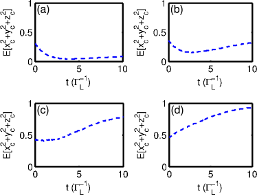
Figure 5: Average purity ${\rm E}\left[{x_{\rm c}^{2}+y_{\rm c}^{2}+z_{\rm c}^{2}}\right]$ over 2000 trajectories. The four plots correspond to the same ensembles calculated in Fig. 4.

The competing effects of sensitivity and back-action in the qubit measurement can be captured by the purity of the conditioned qubit state in the following way. If a pure qubit state remains pure during the measurement, the detector is operating at the quantum limit and can be called an idealKorotkov (1999) detector. In order for the qubit to remain in a pure state once the measurement starts, the SET island must be unoccupied when in steady-state. This occurs when electrons tunnel off the island almost immediately, i.e. when $\Gamma_{\rm L},\Gamma^{\prime}_{\rm L}\ll\Gamma_{\rm R},\Gamma^{\prime}_{\rm R}$. This “asymmetry” adiabatically eliminates the influence of the SET island state on the qubit, as in the model of LABEL:WisetalPRB01. With this condition satisfied, we obtained another ensemble of 2000 quantum trajectories using the conditional master equation and plotted the average purity of the conditioned qubit state in Fig. 6. Note the different y-axis limits. Again the SET response was controlled by changing $\Gamma^{\prime}_{\rm L}$ [again it was decreased incrementally from (a) to (d)]. The SET response was, from (a) to (d), $\Delta I/\bar{I}=0.23$, $0.58$, $1.32$, and $1.70$. Other parameters for Fig. 6 were $\Omega_{0}=0.01\Gamma_{\rm L}$, $\Gamma_{\rm R}=100\Gamma_{\rm L}$, $\Gamma^{\prime}_{\rm R}=100\Gamma_{\rm R}$, $\chi=50\Gamma^{\prime}_{\rm R}$. Similar results were obtained for $\Gamma^{\prime}_{\rm R}=10\Gamma_{\rm R}$. For the strong response plot of Fig. 6 (d), this set of parameters corresponds to the régime given after Eq. (35). That is, the régime where the quantity $\Gamma_{\rm d}\tau_{\rm m}$ approaches 1/2. Indeed, the values of $\Gamma_{\rm d}\tau_{\rm m}$ for Fig. 6 approach this limit of 1/2, as given in the figure caption.

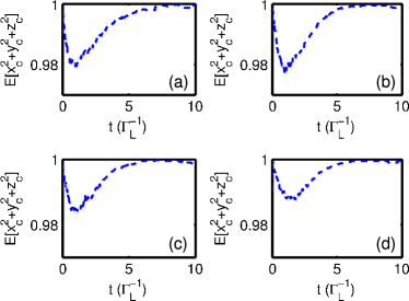
Figure 6: Average purity of the conditioned qubit state, ${\rm E}\left[{x_{\rm c}^{2}+y_{\rm c}^{2}+z_{\rm c}^{2}}\right]$, when monitored by an asymmetric SET ($\bar{\Gamma}_{\rm L}\ll\bar{\Gamma}_{\rm R}$). The average is over 2000 trajectories. Parameter values are given in the text. From (a) to (d), we have $\Gamma_{\rm d}\tau_{\rm m}=1.03$, $0.95$, $0.72$, and $0.59$, respectively.

Figure 6 shows that the average purity of the conditioned qubit state remains very close to 1 throughout the measurement for the asymmetric SET. Thus we can say that the strongly coupled asymmetric SET operates very close to the quantum limit. This conclusion could not be drawn from the values of $\Gamma_{\rm d}\tau_{\rm m}$ alone. Interestingly, the SET response [increasing from plot (a) to (d), as before] has very little effect on a SET with high asymmetry. This is similar to the case of a QPC, which is an ideal detector independent of the strength of its response. To summarize, the conditions required for a strongly coupled SET to operate close to the quantum limit are: (a) $0<\Gamma^{\prime}_{\rm L}\ll\Gamma_{\rm L}$, and (b) $\bar{\Gamma}_{\rm L}\ll\bar{\Gamma}_{\rm R}$.

VI Conclusion

In this paper we have examined sensitivity and back-action in charge qubit measurements by the single-electron transistor (SET) operating in the sequential tunneling mode. We have shown that the unconditional master equations derived in previous workShnirman and Schön (1998); Makhlin et al. (2000, 2001, 2002); Goan (2004) for this measurement (which are equivalent to each other) are not of the Lindblad formLindblad (1976) that is necessary and sufficient for guaranteeing valid physical states. Thus, these master equations cannot be used to model real physical systems. In particular, this statement also applies to the equation for the conditioned state (one that an experimenter would calculate knowing the output of the detector) in LABEL:GoaPRB04. The unconditional master equation was derived independent of the strength of SET-qubit coupling, but analysis of the SET measurement quality (or efficiency) assumedShnirman and Schön (1998); Makhlin et al. (2000, 2001, 2002) weak SET response. Weak response is when the average component of the SET output is much larger than the component that depends on the qubit state.

We have presented an alternative master equation that is of the Lindblad form, as well as the associated quantum trajectory equationCarmichael (1993); Wiseman and Milburn (1993); Wiseman (1996) for the conditioned state. To derive these equations required assuming strong SET-qubit coupling. A strongly coupled detector can exhibit strong response or weak response, whereas weak coupling implies weak response.

We have shown that, in general, quantifying the quality of charge qubit measurements by a SET is not as simple as merely comparing the qubit decoherence (also called coherence) time and measurement time (as done previously for the weakly responding SET in Refs. Shnirman and Schön, 1998, Makhlin et al., 2000, Makhlin et al., 2001, and Makhlin et al., 2002). This is because, for strong SET-qubit coupling, the SET island charge state has a large effect on the qubit coherence. Despite this, comparing qubit decoherence and measurement times does provide some insight into the measurement quality.

Previous definitions for the qubit decoherence timeShnirman and Schön (1998); Makhlin et al. (2000); Korotkov (2001); Makhlin et al. (2001, 2002) either produced an overestimate of the measurement quality (as in Refs. Shnirman and Schön, 1998, Makhlin et al., 2000, Makhlin et al., 2001, and Makhlin et al., 2002), or are only valid for a weakly responding detector (as in LABEL:KorPRB01b). We presented a new definition for the decoherence time that is valid for strong SET-qubit coupling and arbitrary response, by adopting a coherence function techniqueGardiner and Zoller (2000) from the field of quantum optics.

Previous definitions for the measurement timeShnirman and Schön (1998); Makhlin et al. (2000); Korotkov (2001); Makhlin et al. (2001, 2002) are only valid for weakly responding detectors. Thus, we also presented a new definition of the measurement time which is analogous to the new decoherence time definition. Our definition is in terms of the conditioned qubit state, and involves an average over many stochastic measurement records. An analytical approximation for the measurement time compared well to the numerical solution. A similar approach to quantifying the measurement sensitivity was first considered in LABEL:WisetalPRB01.

An important result of this paper was to show that the strongly coupled SET can operate at, or very near, the quantum limit during charge qubit measurements. This was shown in two ways. The first involved comparing the decoherence and measurement times found using our Lindblad-form master equations. In the strong response limit, these times were found to be of the same order as each other. For the highly asymmetric SET where tunneling into the drain (collector) occurs at a much higher rate than tunneling onto the SET from the source (emitter), these times were of the same order as each other, independent of the SET response. This is also the case for the QPC, which can be operated as an ideal detector.Korotkov (1999) The second, and our preferred, way to show that the strongly coupled SET can operate close to the quantum limit was by considering the average qubit purity for an ensemble of stochastic measurement records. Again the asymmetric SET displayed near ideal detector behavior by maintaining the purity of the qubit state above $98\%$.

As far as we are aware, our Lindblad-form quantum trajectory equation is the first of its type presented for charge qubit measurement by a SET. Moreover, having shown that the SET can approach the quantum limit for charge qubit measurements, it is now meaningful to study how the measurement is affected by extra classical noises and filtering due to a realistic measurement circuit.Oxtoby et al. (2003, 2005) This research is continuing.

Appendix A Sensitivity and Back-action in a QPC Measurement

The qubit decoherence rate for measurement by a low-transparency QPC (single tunnel junction device) can be obtained either by inspection of the master equation,Gurvitz (1997); Korotkov (1999); Goan et al. (2001) or using the technique introduced in Sec. IV.1. The same result is obtained using both methods:

$$\Gamma_{\rm d}=\frac{\left({\sqrt{\Gamma}-\sqrt{\Gamma^{\prime}}}\right)^{2}}{2},$$ (36)

where $\Gamma$ ($\Gamma^{\prime}$) is the tunneling rate through the QPC when the target dot is unoccupied (occupied). Using the new technique introduced in Sec. IV.2, the analytical approximation of the qubit measurement time (which agrees with LABEL:GoaMilWisSunPRB01) is

$$\tau^{-1}_{\rm m}=\frac{\left|{\Delta\Gamma}\right|^{2}}{4\bar{\Gamma}}=\frac{\left({\sqrt{\Gamma}+\sqrt{\Gamma^{\prime}}}\right)^{2}}{\Gamma+\Gamma^{\prime}}\Gamma_{\rm d}.$$ (37)

Combining these results gives

$$\Gamma_{\rm d}\tau_{\rm m}=\frac{\Gamma+\Gamma^{\prime}}{\left({\sqrt{\Gamma}+\sqrt{\Gamma^{\prime}}}\right)^{2}}.$$ (38)

Note that $1\geq\Gamma_{\rm d}\tau_{\rm m}\geq 1/2$. The upper bound is approached for a “strongly responding” QPC ($\Gamma\gg\Gamma^{\prime}$). The lower bound is approached for a “weakly responding” QPC ($\Gamma\approx\Gamma^{\prime}$), i.e. when the measurement and decoherence rates go to zero.

Appendix B The SET-qubit Master Equation of Goan

In LABEL:GoaPRB04, Goan presents a master equation for the combined state of the qubit plus island and drain of the SET. In that paper, the master equation is shown to be equivalent to that in LABEL:MakSchShnPRL00. Using our notation and tracing over the drain degrees of freedom gives

$$\dot{G} = -i\left[{\hat{H},G}\right]+\Gamma^{\prime}_{L}{\cal D}\left[{{\hat{b}^{\dagger}\otimes\hat{n}}}\right]G+\Gamma^{\prime}_{R}{\cal D}\left[{{\hat{b}\otimes\hat{n}}}\right]G$$ (39)

$$+\Gamma_{L}{\cal D}\left[{{\hat{b}^{\dagger}\otimes\left({1-\hat{n}}\right)}}\right]G+\Gamma_{R}{\cal D}\left[{{\hat{b}\otimes\left({1-\hat{n}}\right)}}\right]G$$

$$+2\bar{\Gamma}_{\rm L}{\cal D}\left[{{\hat{n}}}\right]\hat{b}^{\dagger}G\hat{b}+2\bar{\Gamma}_{\rm R}{\cal D}\left[{{\hat{n}}}\right]\hat{b}G\hat{b}^{\dagger},$$

where $\hat{b}^{\dagger}$ corresponds to $e^{i\phi}$ in LABEL:GoaPRB04, and we have used $\left[{\hat{n},\left[{\hat{n},\hat{x}}\right]}\right]=-2{\cal D}\left[{{\hat{n}}}\right]\hat{x}$. This master equation is equivalent to those in Refs. Shnirman and Schön, 1998, Makhlin et al., 2000, Makhlin et al., 2001, and Makhlin et al., 2002. Comparison of this equation with our unconditional master equation (19) shows that the terms in the final line of Eq. (39) are not present in our model. These are the terms that lead to the non-Lindbladian dynamics in Refs. Shnirman and Schön, 1998, Makhlin et al., 2000, and Makhlin et al., 2001, 2002; Goan, 2004.

References

- Averin and Likharev (1986) D. V. Averin and K. K. Likharev, J. Low Temp. Phys. 62, 345 (1986).
- Fulton and Dolan (1987) T. A. Fulton and G. J. Dolan, Phys. Rev. Lett. 59, 109 (1987).
- Shnirman and Schön (1998) A. Shnirman and G. Schön, Phys. Rev. B 57, 15400 (1998).
- Devoret and Schoelkopf (2000) M. H. Devoret and R. J. Schoelkopf, Nature 406, 1039 (2000).
- Nielsen and Chuang (2000) M. A. Nielsen and I. L. Chuang, Quantum Computation and Quantum Information (Cambridge University Press, Cambridge, U.K., 2000).
- Field et al. (1993) M. Field, C. G. Smith, M. Pepper, D. A. Ritchie, J. E. F. Frost, G. A. C. Jones, and D. G. Hasko, Phys. Rev. Lett. 70, 1311 (1993).
- Korotkov (1999) A. N. Korotkov, Phys. Rev. B 60, 5737 (1999).
- Braginsky and Khalili (1992) V. B. Braginsky and F. Y. Khalili, Quantum Measurement (Cambridge University Press, 1992).
- Gurvitz (1997) S. A. Gurvitz, Phys. Rev. B 56, 15215 (1997).
- Goan et al. (2001) H.-S. Goan, G. J. Milburn, H. M. Wiseman, and H. B. Sun, Phys. Rev. B 63, 125326 (2001).
- Pilgram and Büttiker (2002) S. Pilgram and M. Büttiker, Phys. Rev. Lett. 89, 200401 (2002).
- Makhlin et al. (2000) Y. Makhlin, G. Schön, and A. Shnirman, Phys. Rev. Lett. 85, 4578 (2000).
- Korotkov (2001) A. N. Korotkov, Phys. Rev. B 63, 115403 (2001).
- Makhlin et al. (2001) Y. Makhlin, G. Schön, and A. Shnirman, Rev. Mod. Phys. 73, 357 (2001).
- Makhlin et al. (2002) Y. Makhlin, G. Schön, and A. Shnirman, in Exploring the Quantum-Classical Frontier, edited by J. R. Friedman and S. Han (Nova Science, Commack NY, USA, 2002), pp. 405 – 440.
- Goan (2004) H.-S. Goan, Phys. Rev. B 70, 075305 (2004).
- Lindblad (1976) G. Lindblad, Comm. Math. Phys. 48, 199 (1976).
- Carmichael (1993) H. J. Carmichael, An Open Systems Approach to Quantum Optics (Springer, Berlin, 1993).
- Wiseman and Milburn (1993) H. M. Wiseman and G. J. Milburn, Phys. Rev. A 47, 1652 (1993).
- Wiseman (1996) H. M. Wiseman, Quantum Semiclass. Opt. 8, 205 (1996).
- Belavkin (1980) V. P. Belavkin, Radiotechnika and Electronika 25, 1445 (1980).
- Belavkin (1995) V. P. Belavkin, in Quantum Communications and Measurement, edited by V. P. Belavkin, O. Hirota, and R. L. Hudson (Plenum Press, New York, 1995), pp. 381–392.
- Hayashi et al. (2003) T. Hayashi, T. Fujisawa, H. D. Cheong, Y. H. Jeong, and Y. Hirayama, Phys. Rev. Lett. 91, 226804 (2003).
- Schoelkopf et al. (2003) R. J. Schoelkopf, A. A. Clerk, S. M. Girvin, K. W. Lehnert, and M. H. Devoret, in Noise and Information in Nanoelectronics, Sensors and Standards, edited by L. B. Kish, F. Green, G. Iannaccone, and J. R. Vig (SPIE, 2003), vol. 5115, pp. 356–376.
- Korotkov (1994) A. N. Korotkov, Phys. Rev. B 49, 10381 (1994).
- van Houten et al. (1992) H. van Houten, C. W. J. Beenakker, and A. A. M. Staring, in Single Charge Tunneling: Coulomb Blockade Phenomena in Nanostructures, edited by H. Grabert and M. H. Devoret (Plenum Press, New York, 1992), vol. 294 of NATO ASI Series B.
- Wiseman et al. (2001) H. M. Wiseman, D. W. Utami, H. B. Sun, G. J. Milburn, B. E. Kane, A. Dzurak, and R. G. Clark, Phys. Rev. B 63, 235308 (2001).
- Korotkov (2003) A. N. Korotkov, in Quantum Noise in Mesoscopic Physics, edited by Y. V. Nazarov (Kluwer Academic, Netherlands, 2003), pp. 205–228.
- Glauber (1963) R. J. Glauber, Phys. Rev. 130, 2529 (1963).
- Gardiner and Zoller (2000) C. W. Gardiner and P. Zoller, Quantum Noise (Springer, Berlin, 2000), 2nd ed.
- Beenakker (1991) C. W. J. Beenakker, Phys. Rev. B 44, 1646 (1991).
- Gardiner (1985) C. W. Gardiner, Handbook of Stochastic Methods for the Physical Sciences (Springer, Berlin, 1985).
- Oxtoby et al. (2003) N. P. Oxtoby, H.-B. Sun, and H. M. Wiseman, J. Phys.: Condens. Matter 15, 8055 (2003).
- Oxtoby et al. (2005) N. P. Oxtoby, P. Warszawski, H. M. Wiseman, H.-B. Sun, and R. E. S. Polkinghorne, Phys. Rev. B 71, 165317 (2005).
- Doherty et al. (2001) A. C. Doherty, K. Jacobs, and G. Jungman, Phys. Rev. A 63, 062306 (2001).
- Fuchs and Jacobs (2001) C. A. Fuchs and K. Jacobs, Phys. Rev. A 63, 062305 (2001).
- Korotkov (2000) A. N. Korotkov, Physica B 280, 412 (2000).