Electron-like and photon-like excitations in an ultracold Bose-Fermi atom mixture

Abstract

We show that the electron-like and photon-like excitations may exist in a three-dimensional Bose-Fermi Hubbard model describing ultracold Bose-Fermi atom mixtures in optical lattices. In a Mott insulating phase of the Bose atoms, these excitations are stabilized by an induced repulsive interaction between ’electrons’ if the Fermi atoms are nearly half filling. We suggest to create ’external electric field’ so that the electron-like excitation can be observed by measuring the linear density-density response of the ’electron’ gas to the ’external field’ in a time-of-flight experiment of the mixture. The Fermi surface of the ’electron’ gas may also be expected to be observed in the time-of-flight.

Ultracold atoms in optical lattices have offered a highly tunable platform to study various physical phenomena which may not be definitely clarified in condensed matter systems exa . On the other hand, new systems which may not be realized in condensed matter content are presented, for example, mixtures of Bose-Fermi atoms as constitution particles. Experimentally, the Bose-Fermi atom mixtures in optical lattices have been realized for ⁸⁷Rb-⁴⁰K rbk , and ²³Na-⁶Li nali .

Microscopically, these mixtures may be described by a Bose-Fermi Hubbard model aie . The constitution particles in this model are spinless boson($a_{i}$) and fermion ($f_{i}$) with $i$ the lattice site index. In this Letter, we consider three-dimensional cubic lattices. We will show that, in high temperatures, there are only excitations of these constitution particles. We call this a confinement phase. The system undergoes a phase transition, in certain critical temperature, to a uniform mean field (UMF) state in which electron-like and photon-like excitations emerge if the fermion occupation is nearly half filling wen . At the exact half filling, this UMF state turns to a long range ordered state, the checkerboard crystal of ’electrons’ comp . We show that this UMF state can only be stable if the bosons are in a Mott insulator (MI) ground state.

We suggest an experiment to create an ’external field’ by changing the depth of the fermion’s optical potential change . The response function of the mixture to the external field may be measured by the density distribution image in a time-of-flight of the mixture cloud. The behavior of the response functions may be used to identify the electron-like excitation. We expect the ’electron’ Fermi surface can be observed by the time-of-flight experiment, which has been used to observe the Fermi surface of the pure cold Fermi atoms kms .

The Bose-Fermi Hubbard Hamiltonian we are interested in reads

$$H = -\sum_{\langle ij\rangle}(t_{B}a^{\dagger}_{i}a_{j}+t_{F}f^{\dagger}_{i}f_{j})-\sum_{i}(\mu_{B}n^{a}_{i}+\mu_{F}n^{f}_{i})$$ (1)

$$+ \frac{U_{BB}}{2}\sum_{i}n^{a}_{i}(n^{a}_{i}-1)+U_{BF}\sum_{i}n^{a}_{i}n^{f}_{i},$$

where the lattice spacing $\lambda/2$ is set to unit. ( We also set $\hbar=c=1$.) $n^{a}_{i}=a^{\dagger}_{i}a_{i}$ and $n^{f}_{i}=f^{\dagger}_{i}f_{i}$. $t_{B}$ and $t_{F}$ are the hopping amplitudes of the boson and fermion between a pair of nearest neighbor sites $\langle ij\rangle$. $\mu_{B}$ and $\mu_{F}$ are chemical potentials. And $U_{BB}$ and $U_{BF}$ are the on-site interactions between bosons, and between boson and fermion. In this work, we use $U_{BB}>U_{BF}>0$ although this is not necessary in general. The microscopic calculations of these model parameters in terms of the cold atom mixture have been established, e.g, in Ref. aie .

To deduce the low energy theory in strong couplings, we will use the slave particle technique, which has been applied to the cold boson system d ; yu ; lu . In the slave particle language, the Hamiltonian reads $H=H_{2}+H_{4}$ where $H_{2}$ and $H_{4}$ are the two-operator and four-operator terms, respectively. Namely,

$$H_{2}=-\sum_{i}\sum_{\alpha}[\mu_{B}\alpha(n^{\alpha}_{c,i}+n^{\alpha}_{h,i})+\mu_{F}n^{\alpha}_{c,i}]$$ (2)

$$+\frac{U_{BB}}{2}\sum_{i}\sum_{\alpha}\alpha(\alpha-1)(n_{c,i}^{\alpha}+n_{h,i}^{\alpha})+U_{BF}\sum_{i}\sum_{\alpha}\alpha n_{c,i}^{\alpha},$$

and

$$H_{4} = -\sum_{\langle ij\rangle}t_{F}\sum_{\alpha,\beta}c^{\dagger}_{\alpha,i}h_{\alpha,i}h^{\dagger}_{\beta,j}c_{\beta,j}$$

$$- \sum_{\langle ij\rangle}t_{B}\sum_{\alpha,\beta}\sqrt{\alpha+1}\sqrt{\beta+1}$$

$$( h^{\dagger}_{\alpha+1,i}h_{\alpha,i}+c^{\dagger}_{\alpha+1,i}c_{\alpha,i})(h^{\dagger}_{\beta,j}h_{\beta+1,j}+c^{\dagger}_{\beta,j}c_{\beta+1,j}),$$

where $n^{\alpha}_{c,i}=c^{\dagger}_{\alpha,i}c_{\alpha,i}$ and $n^{\alpha}_{h,i}=h^{\dagger}_{\alpha,i}h_{\alpha,i}$. We explain briefly the derivation of this slave particle Hamiltonian. The state configurations at an arbitrary given site consists of $\{|\alpha,s\rangle~{}|~{}\alpha=0,1,2,...~{};~{}s=0,1\}$ where $\alpha$ and $s$ are the boson and fermion occupations, respectively. The Bose and Fermi creation operators can be expressed as $a^{\dagger}=\sum_{\alpha}\sqrt{\alpha+1}[|\alpha+1,0\rangle\langle\alpha,0|+|\alpha+1,1\rangle\langle\alpha,1|],f^{\dagger}=\sum_{\alpha}|\alpha,1\rangle\langle\alpha,0|$. The mapping to the slave particle reads $|\alpha,0\rangle\to h^{\dagger}_{\alpha},|\alpha,1\rangle\to c^{\dagger}_{\alpha}$ . We call $c_{\alpha}$ the composite fermion (CF) comp and $h_{\alpha}$ the slave boson. The normalized condition $\sum_{\alpha}(|\alpha,0\rangle\langle\alpha,0|+|\alpha,1\rangle\langle\alpha,1|)=1$ implies a constraint $\sum_{\alpha}(n^{\alpha}_{c}+n^{\alpha}_{h})=1$ at each site. The slave particles arise a $U(1)$ gauge symmetry $c_{\alpha,i}\to e^{i\varphi_{i}}c_{\alpha,i},h_{\alpha,i}\to e^{i\varphi_{i}}h_{\alpha,i}.$ The global $U(1)$ symmetry $c_{\alpha,i}\to e^{i\alpha\varphi}c_{\alpha,i},h_{\alpha,i}\to e^{i\alpha\varphi}h_{\alpha,i}$ reflects the particle number conservation. Since the slave particle technique essentially works in the strong coupling region, we focus on $U_{BB}/(6t_{B})\gg 1$.

There are two types of four slave particle terms in $H_{4}$, the $t_{B}$-terms and $t_{F}$-terms. We first neglect the $t_{B}$-terms in the mean field level of the CF. To decouple the $t_{F}$-terms , we introduce Hubbard-Stratonovich fields $\hat{\eta}^{c,h}_{\alpha\beta,ij}$ and $\hat{\chi}^{c,h}_{\alpha\beta,ij}$. The partition function is given by $Z=\int D\hat{\chi}D\hat{\eta}D\bar{c}DcD\bar{h}DhD\Lambda~{}e^{-S_{eff}}$ where the effective action reads

$$S_{eff}[\hat{\chi},\hat{\eta},c,h,\Lambda]=\int_{0}^{1/T}d\tau\biggl{\{}H_{2}+\sum_{i}i\Lambda_{i}$$

$$+\sum_{i}\sum_{\alpha}\biggl{[}\bar{c}_{\alpha,i}(\partial_{\tau}-i\Lambda_{i})c_{\alpha,i}+\bar{h}_{\alpha,i}(\partial_{\tau}-i\Lambda_{i})h_{\alpha,i}\biggr{]}$$

$$+\sum_{\langle ij\rangle;\alpha,\beta}t_{F}[\hat{\eta}^{h}_{\beta\alpha,ji}(\hat{\chi}^{c}_{\alpha\beta,ij}-\bar{c}_{\alpha,i}c_{\beta,j})-\hat{\chi}^{c}_{\alpha\beta,ij}\hat{\chi}^{h}_{\beta\alpha,ji}$$

$$+\hat{\eta}^{c}_{\alpha\beta,ij}(\hat{\chi}^{h}_{\beta\alpha,ji}-\bar{h}_{\beta,j}h_{\alpha,i})]+t_{B}~{}{\rm terms}\biggr{\}},$$ (4)

where $\Lambda_{i}$ is a Lagrange multiplier for the constraint $\sum_{\alpha}(n^{\alpha}_{c,i}+n^{\alpha}_{h,i})=1$. Rewriting $\hat{\eta}^{c,h}_{\alpha\beta,ij}=\eta^{c,h}_{\alpha\beta,ij}e^{i{\cal A}_{ij}}$, $\hat{\chi}^{c,h}_{\alpha\beta,ij}=\chi^{c,h}_{\alpha\beta,ij}e^{i{\cal A}_{ij}}$ and $\Lambda_{i}=\Lambda+{\cal A}_{0,i}$, ${\cal A}_{0i}$ and ${\cal A}_{ij}$ are $U(1)$ gauge field corresponding to the gauge symmetry tj . Before going to a mean field state, we first require the mixture is stable against the Bose-Fermi phase separation. For example, it was known that the mixture is stable in the MI phase if $4\pi t_{F}\sin(\pi n^{f})U_{BB}>U_{BF}^{2}$ aie . Near the half filling of Fermi atoms, this condition is easy to be satisfied. Fixing a gauge, $\hat{\eta}_{\alpha\beta,ij}^{h}\approx\eta^{h}_{\alpha\beta,ij}$, $\hat{\chi}_{\alpha\beta,ij}^{h}\approx\chi^{h}_{\alpha\beta,ij}$ and $\Lambda_{i}\approx\Lambda$ (which is a saddle point value of $\Lambda_{i}$). This is corresponding to a mean field approximation. The effective mean field action is given by

$$S_{MF} = iN_{s}\beta\Lambda+\int d\tau\biggl{\{}\sum_{\langle ij\rangle}(t_{F}\sum_{\alpha\beta}\chi^{c}_{\alpha\beta,ij}\chi^{h}_{\beta\alpha,ji})$$

$$+ \sum_{i\neq j}\sum_{\alpha\beta}(\bar{c}_{\alpha,i}(D^{\alpha\beta}_{c})^{-1}_{ij}c_{\beta,j}+\bar{h}_{\alpha,i}(D^{\alpha\beta}_{h})^{-1}_{ij}h_{\beta,j})\biggr{\}}$$

where $(D^{\alpha\beta}_{c})^{-1}_{ij}=(\partial_{\tau}-\mu^{\alpha}_{F})\delta_{ij}\delta_{\alpha\beta}-t_{F}\sum_{\vec{\tau}}\chi^{h}_{\alpha\beta,ji}\delta_{j,i+\vec{\tau}}$ with $\mu^{\alpha}_{F}=\mu_{B}\alpha+\mu_{F}-\frac{U_{BB}}{2}\alpha(\alpha-1)-U_{BF}\alpha-i\Lambda$ and $(D^{\alpha\beta}_{h})^{-1}_{ij}==(\partial_{\tau}-\mu^{\alpha}_{B})\delta_{ij}\delta_{\alpha\beta}-t_{F}\sum_{\vec{\tau}}\chi^{c}_{\alpha\beta,ji}\delta_{j,i+\vec{\tau}}$. with $\mu_{B}^{\alpha}=\mu_{B}\alpha-\frac{U_{BB}}{2}\alpha(\alpha-1)-i\Lambda$. ($\vec{\tau}$ is the unit vector of the lattice.)

The mean field equations are $\chi^{c}_{\alpha\beta,ij}=\langle c^{\dagger}_{\alpha,i}c_{\beta,j}\rangle=T\sum_{n}D^{\alpha\beta}_{c,ij}(p_{n}),\chi^{h}_{\alpha\beta,ij}=\langle h^{\dagger}_{\alpha,i}h_{\beta,j}\rangle=T\sum_{n}D^{\alpha\beta}_{h,ij}(\omega_{n})$ where $D^{\alpha\beta}_{c,ij}(p_{n})=\int d\tau e^{ip_{n}\tau}D^{\alpha\beta}_{c,ij}(\tau)$ and $D^{\alpha\beta}_{h,ij}(\omega_{n})=\int d\tau e^{i\omega_{n}\tau}D^{\alpha\beta}_{h,ij}(\tau)$ with $p_{n}$ and $\omega_{n}$ the Fermi and Bose frequencies. Near the critical point where $\chi^{h,c}_{\alpha\beta,ij}\approx 0$, one can expand $D_{i\neq j}^{\alpha\beta}$ by $\chi^{h,c}_{\alpha\beta,ij}$. For $\alpha\neq\beta$, the mean field equations are $\chi_{\alpha\beta,ij}^{c}=t_{F}\chi_{\beta\alpha,ji}^{h}\frac{n_{c}^{\alpha}-n_{c}^{\beta}}{\mu_{F}^{\alpha}-\mu_{F}^{\beta}}$ and $\chi_{\alpha\beta,ij}^{h}=t_{F}\chi_{\beta\alpha,ji}^{c}\frac{n_{h}^{\alpha}-n_{h}^{\beta}}{\mu_{B}^{\alpha}-\mu_{B}^{\beta}}$ with $n_{h}^{\alpha}=[e^{-\beta\mu_{B}^{\alpha}}-1]^{-1},n_{c}^{\alpha}=[e^{-\beta\mu_{F}^{\alpha}}+1]^{-1}$. The solutions of these mean field equations can only exist in the weak coupling limit, i.e., $\mu_{F,B}^{\alpha}\ll t_{F}$: $T_{c}^{\alpha\beta}=t_{F}$. Therefore, in the parameters we are considering, $\chi_{\alpha\beta,ij}^{h,c}=0$ for $\alpha\neq\beta$. For $\alpha=\beta$, the mean field equations are $T^{\alpha}_{c}\chi_{\alpha\alpha,ij}^{c}=T^{\alpha}_{F}\chi_{\alpha\alpha,ji}^{h}$ and $T^{\alpha}_{c}\chi_{\alpha\alpha,ij}^{h}=T^{\alpha}_{B}\chi_{\alpha\alpha,ji}^{c}$ with $T^{\alpha}_{F,B}=t_{F}n^{\alpha}_{c,h}(1\mp n^{\alpha}_{c,h})$. The critical temperatures are then given by $T_{c}^{\alpha}=\sqrt{T^{\alpha}_{F}T^{\alpha}_{B}}.$ Below $T_{c}^{\alpha}$, the minimized free energy including variables $\chi_{\alpha\alpha}^{h,c}$ is $F\propto-t_{F}\sum_{\alpha}(\tau^{\alpha})^{2}\frac{(S^{\alpha}_{2})^{2}}{S^{\alpha}_{4}}$ where $\tau^{\alpha}=\frac{T^{\alpha}_{c}-T}{T}$ and $S^{\alpha}_{2}$, $S^{\alpha}_{4}$ are the fractions of non-zero terms corresponding to the second order and four order of $|\chi_{\alpha\alpha}|$ il . The optimal $|\chi^{c}_{\alpha\alpha}|^{2}\propto\tau^{\alpha}S^{\alpha}_{2}/S^{\alpha}_{4}$.

We consider an integer boson filling $n^{a}=$1 for $\bar{U}_{BB}\gg 1$. Since $n^{\alpha\neq 1}_{h}$ and $n^{\alpha\neq 1}_{c}$ in this region are very small, there are no solutions of the mean field equations with $T^{\alpha\neq 1}_{c}\geq 0$ for the critical temperature equations. Thus, all slave bosons and CFs with $\alpha\neq 1$ are confined. Only $T^{1}_{c}>0$ can be found. Below $T_{c}^{1}$, the CF $c_{1}$ and the slave boson $h_{1}$ are deconfined in the mean field sense. In the inset of Fig. 1, we plot $T_{c}^{1}$ for a set of given parameters. The curve $T_{p}(U_{BB})$ is corresponding to $\mu^{1}_{F}(T_{p})=0$, i.e., the effective chemical potential of $c_{1}$ vanishes.

We now go to concrete mean field solutions and focus on the near half filling of the fermions. Because we work in a three-dimensional lattice, the flux quanta passing a cubic cell are zero. Thus, there is no a flux mean field state. (The flux mean field state may exist in a two-dimensional Bose-Fermi Hubbard model.) Two possible solutions are the dimer and uniform phases. In a cubic lattice, each lattice site has six nearest neighbor sites. A pair of slave boson and CF located at the nearest neighbor sites may form a bond. The dimer phase means for any given site, only one bond ended at the site is endowed with a non-zero $\chi_{\alpha\alpha}^{h,c}$ and other five bond carry $\chi_{\alpha\alpha}^{h,c}=0$. In the uniform phase, each bond is endowed with the same real values of $\chi^{c,h}_{\alpha}$ if a CF (i.e., $a_{i}^{\dagger}f_{i}^{\dagger}|0\rangle=c^{\dagger}_{1i}|{\rm vac}\rangle$) is surrounded by six slave bosons (e.g., $a_{j}^{\dagger}|0\rangle=h^{\dagger}_{1j}|{\rm vac}\rangle$). In the fermion half filling, this is a CF checkerboard crystal state comp . Slightly away from the half filling, this is a UMF state with $h_{1}$-$c_{1}$ bond. In the uniform phase, the dispersions of the CFs and slave bosons are $\xi_{\alpha}^{c,h}(k)=t_{F}|\chi_{\alpha}^{h,c}||\sum_{i}\cos k_{i}|$.

At the fermion half filling, the mean field free energy favors for the dimer state. However, as we shall see soon, in the Mott insulator phase of the bosons, the boson hopping term ($t_{B}$-term) we have neglected at the mean field level will contribute a nearest neighbor repulsion between CFs or slave bosons if $U_{BB}>U_{BF}$. This repulsion potential will raise the energy of dimer phase while the uniform phase is not affected. Thus, for our purpose, we focus on the uniform phase below.

In the mean field approximation, we neglect the boson hopping term and the gauge fluctuations ${\cal A}_{0i}$, ${\cal A}_{ij}$ which must be considered if the mean field state is stable. We first deal with the $t_{B}$-term. Introduce a Hubbard-Stratonovich field $\Phi_{i}=\sum_{\alpha}\sqrt{\alpha+1}[c^{\dagger}_{\alpha+1,i}c_{\alpha,i}+h^{\dagger}_{\alpha+1,i}h_{\alpha,i}]$ to decouple $t_{B}$-term. $\Phi_{i}$ may be thought as the order parameter field of the Bose condensation. The phase diagram of the boson may be determined by minimizing the Landau free energy associated with the order parameter $\langle 0|\Phi_{i}|0\rangle$. The vanishing of the coefficient of the second order term in the free energy gives the phase boundary d ; yu . It has to point out that here the fluctuation ${\cal A}_{0i}$ has been neglected and a cut-off to the type of the slave bosons has to be introduced. However, the experience to work out the pure Bose phase diagram showed that these approximations could be acceptable d ; yu ; lu .

As expected, the phase diagram of the constitution boson consists of the Bose superfluid (BSF), the normal liquid and the MI, in which the MI phase only exists in the zero temperature and an integer boson filling factor . In the inset of Fig. 1, we show the boson phase diagram in the same parameters as those in the CF mean field phase diagram. In the Bose condensate, the boson number in each site is totally uncertainty. This means the vanishing bond number or $S_{2}\approx S_{4}\approx 0$. Thus, the mean field state is not stable in the BSF. In the MI phase of the bosons, on the other hand, the boson number in each site is exactly one for $n^{a}=1$. Thus, the mean field states may be stable. Furthermore, the $t_{B}$-term induces a nearest neighbor interaction between CFs or slave bosons. This may be seen by taking the $t_{B}$ term as a perturbation if $U_{BB}$ and $U_{BB}-U_{BF}$ are much larger than $t_{B}$. To the second order of the perturbation, the $t_{B}$-term contributes an effective repulsive interaction between the CFs or slave bosons in the nearest neighbor sites

$${\cal J}=\sum_{\langle ij\rangle}Jn^{1}_{ci}n^{1}_{cj}+{\rm const}=\sum_{\langle ij\rangle}Jn^{1}_{hi}n^{1}_{hj}+{\rm const^{\prime}},$$ (6)

with $J=\frac{16t_{B}^{2}U_{BF}^{2}}{U_{BB}(U_{BB}^{2}-U_{BF}^{2})}$. For the dimer state, this repulsive potential contributes an energy $J/2$ to a pair of adjacent bonds. For the UMF state, if the fermion is in half filling, the checkerboard distribution of the fermions (then CFs) makes ${\cal J}$ no contribution to the energy. For a doping $\delta$, i. e., slightly away from the half filling, the energy raises a small amount of the order $J\delta$. Thus, the UMF state minimizes this induced nearest neighbor repulsion.

We have shown the mean field states are not stable in the BSF. Therefore, we focus on the MI phase of the bosons below and examine the gauge fluctuations. The zeroth component ${\cal A}_{i0}$ restores the exact constraint of one type of slave particles per site while ${\cal A}_{ij}$ restores the gauge invariance of the effective action (4). These fluctuations may destabilize the mean field state. To see the stability of the UMF state against the gauge fluctuation, one should integrate out $h_{1}$ and $c_{1}$. In the long wave length limit ($k\to 0$), integrating out $h_{1}$ first and keeping the Gaussian fluctuations of the gauge field, an effective action in continuum limit is given by

$$S[c_{1},A_{\mu}]=T\sum_{n}\int d^{3}k\biggl{[}\bar{c}_{1}(ip_{n}-\mu_{c}^{1}+ie_{0}A_{0})c_{1}$$ (7)

$$+\frac{1}{2m_{c}}\bar{c}_{1}(k_{a}+ie_{0}A_{a})^{2}c_{1}+\frac{1}{2}A_{\mu}A_{\nu}\Pi^{B}_{\mu\nu}(k,\omega_{n})\biggr{]},$$

where $e_{0}=\sqrt{\frac{J}{4\pi}}$, $A_{\mu}={\cal A}_{\mu}/e_{0}$, $m_{c}\sim 1/(t_{F}\chi^{c}_{1}\delta)$ is the effective mass of CF. The coupling constant $2\pi e_{0}^{2}=J/2$ is a small quantity means that the Gaussian approximation to the gauge field is reasonable. $\Pi^{B}_{\mu\nu}$ is the response function by integrating over $h_{1}$. The density-density response function is given by $[\Pi^{B}_{00}(\omega,k)]^{-1}=[\Pi^{B(0)}_{00}(\omega,k)]^{-1}+V(k)$ where $V(k)=J\sum_{a}(1-k^{2}/2)$ is the Fourier component of the interaction (6) and $\Pi^{B(0)}_{00}(\omega,k)$ is the free boson response function. The current-current response function has a form $\Pi^{B}_{ij}=(\delta_{ij}-k_{i}k_{j}/k^{2})\Pi^{B}_{L}+(k_{i}k_{j}/k^{2})\Pi^{B}_{T}$. In the long wave length limit, the transverse part $\Pi^{B}_{T}=-\frac{\omega^{2}}{k^{2}}\Pi^{B}_{00}$. The longitudinal part $\Pi^{B}_{L}(k,\omega)\propto|\langle 0|h_{1}|0\rangle|^{2}$ as $k,\omega\to 0$. However, out of the BSF phase, $h_{1}$ does not condense. Thus, $A_{\mu}$ is a transverse field and the action (7) is very similar to electron coupled to a photon field. We, therefore, call $c_{1}$ and $A_{\mu}$ the electron-like and photon-like excitation, respectively. Since the hopping of the Bose atom in the optical lattice is short range, the repulsive interaction between ’electrons’ is also short range. If it was possible to design the hopping of bosons $t_{B,ij}\propto 1/\sqrt{|{\bf i}-{\bf j}|}$, the interaction between ’electrons’ would be purely coulombic, i.e., $V(k)\propto 1/k^{2}$. The stability of the UMF state against to the gauge fluctuations may be seen after integrating out $c_{1}$ field. This leads to a CF response function $[\Pi^{F}_{\mu\nu}(\omega_{n},k)]^{-1}=[\Pi^{F(0)}_{\mu\nu}(\omega_{n},k)]^{-1}+[\Pi^{B}_{\mu\nu}(\omega_{n},k)]^{-1}$. The UMF is stable when $\Pi^{F}_{\mu\nu}(0,0)>0$. In the long wave length limit, it is positive if $6J>\frac{\pi^{2}}{m_{c}k_{F}^{1}}$ where $k_{F}^{1}$ is Fermi momentum of the CF. Since $1/m_{c}\propto t_{F}\delta$, this condition holds only when the fermion filling is slightly away from the half filling.

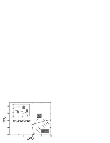
Figure 1: The phase diagram of the CFs in the $U_{BB}$-$T$ plane for $n^{a}=1$, $U_{BF}=U_{BB}/2$, $t_{F}/6t_{B}=\sqrt{60}$, $n^{f}=0.55$. The solid curves are the critical temperature $T^{1*}_{c}$ after considering the gauge fluctuation and the shrink of the CF Fermi surface.

We have shown the stability of the UMF state near the fermion half filling when the bosons are in the MI phase. We may figure out the phase diagram of the CF in Fig. 1. The mean field phase transition temperature $T_{c}^{1}$ is suppressed greatly to $T_{c}^{1*}$ which is determined by the $T_{c}$ and $T_{p}$. The dash line is the estimated crossover line from the ’electron’ gas (the MI of bosons) to the Fermi liquid of the constitution Fermi atoms (the normal liquid of bosons as the incompressibility of the MI is gradually disappearing).

The experimental implications of the UMF phase are discussed as follows. We consider the ’electron’ response to an external ’electric’ field, ’made’ by a change of the lattice potential of the Fermi atoms. This technique has been used to study the excitation spectrum of atom superfluid in optical lattices change . This disturbs the density of Fermi atoms with $H^{\prime}=-\sum_{i}n^{f}_{i}\varphi_{i}$. In a time-of-flight experiment, the difference between disturbed and undisturbed fermion densities by external field is given by $n_{f}({\bf r})-n^{0}_{f}({\bf r})=(\frac{m_{f}}{t})|\tilde{w}_{f}({\bf k}=\frac{m_{f}{\bf r}}{t})|^{2}\delta n_{f}({\bf k}=\frac{m_{f}{\bf r}}{t})$ where $n_{f}({\bf r})$ is the image after the time-of-flight and $n_{f}({\bf k})$ is the Fourier component of $n_{i}^{f}$; $t$ is the flying time, $\tilde{w}_{f}$ is the Fourier component of the fermion Wannier function and $m_{f}$ the Fermi atom mass. If $T>T_{c}^{1*}$, the density response of the system is simply given by the free fermion one, and then $\delta n_{f}({\bf k})\propto\Pi^{F(0)}_{00}$. When the bosons are in the MI phase ($n^{a}_{i}=1$), $n^{f}_{i}=n^{1}_{ci}$ implies $\delta n^{f}({\bf k})=\delta n^{1}_{c}({\bf k})$. Thus, for $T<T^{1*}_{c}$, especially below the dash line in Fig. 1, $\delta n_{f}({\bf k})\propto\Pi_{00}({\bf k},0)$ with $\Pi_{00}^{-1}=(\Pi^{F(0)}_{00})^{-1}+(\Pi^{B(0)}_{00})^{-1}+V(k)$. Then, this difference between the response functions may be measured in experiment. A better experimentally measurable quantity is the visibility ${\cal V}=\frac{n_{f}({\bf r}_{\rm max})-n_{f}({\bf r}_{\rm min})}{n_{f}({\bf r}_{\rm max})+n_{f}({\bf r}_{\rm min})}$ where ${\bf r}_{\rm max}$ and ${\bf r}_{\rm min}$ are chosen such that the Wannier envelop is cancelled vi . The difference between the disturbed and undisturbed visibility may directly correspond to the response function because $n_{f}({\bf r}_{\rm max})+n_{f}({\bf r}_{\rm min})\approx n^{0}_{f}({\bf r}_{\rm max})+n^{0}_{f}({\bf r}_{\rm min})$ in denominator. To directly see the image of the fermion cloud, one may use a magnetic field to separate the fermion cloud from boson cloud before recording the fermion image in the time-of-flight as splitting components in a spinor Bose atom condensate sp .

The Fermi surface of pure cold fermions has been observed in a recent experiment kms by the time-of-flight experiment. When the mixture in the UMF state, as we have discussed in the previous paragraph, $n_{f}({\bf r})=(\frac{m_{f}}{t})|\tilde{w}_{f}({\bf k})|^{2}n_{c}^{1}({\bf k}=\frac{m_{f}{\bf r}}{t})$. Therefore, it is expected that instead of the Fermi surface of the free Fermi atoms, one may observe the ’electron’ Fermi surface of the ’electron’ gas. Namely, in the image of the time-of-flight, most of Fermi atoms are inside of area with $|{\bf r}|<|{\bf k}_{F}^{1}|t/m_{f}$ but not $|{\bf r}|<|{\bf k}_{F}|t/m_{f}$ ( $|{\bf k}_{F}|$ is Fermi surface of the free Fermi atoms.).

In conclusions, we showed that there may be electron-like and photon-like excitations in mixtures of Bose-Fermi atoms in optical lattices in which the bosons are in the MI phase ($U_{BB}$ and $U_{BB}-U_{BF}\gg t_{B}$) and the fermions are nearly half filling. (To avoid the demixing, $4\pi t_{F}\sin(\pi n^{f})U_{BB}>U_{BF}^{2}$.) It was suggested that through the time-of-flight experiment, the electron-like response function and the ’electron’ Fermi surface may be measured. An electron-like response function also implies a gauge field effect. However, an experiment how to directly observe a ’photon’ was not designed yet.

This work was supported in part by Chinese National Natural Science Foundation and the NSF of USA.

References

• (1) For examples, see, C. Orzel, A. K. Tuchman, M. L. Fenselau, M. Yasuda, and M. A. Kasevich Science 291 2386 (2001).M. Greiner, O. Mandel, T. Esslinger, T. W. Hänsch, and I. Bloch, Nature (London) 415, 39 (2002). D. Jaksch, C. Bruder, J. I. Cirac, C. W. Gardiner and P. Zoller, Phys. Rev. Lett. 81, 3108 (1998).
• (2) G. Modugno et al, Phys. Rev. A 68, 011601(R) (2003). C. Schori et al, Phys. Rev. Lett 93, 240402 (2004). S. Inouye et al, Phys. Rev. Lett. 93, 183201 (2004). J. Goldwin et al, Phys. Rev. A 70, 021601(R) (2004).
• (3) C. A. Stan et al, Phys. Rev. Lett. 93 143001 (2004).
• (4) A. Albus, F. Illuminati, J. Eisert, Phys. Rev. A 68, 023606 (2003).
• (5) For emergence of ’Photon’ and ’electron’ from a non-relativistic model, see, e.g., P. A. Lee, N. Nagaosa, X. G. Wen, cond-mat/0410445 and references therein.
• (6) M. Lewenstein, L. Santos, M. A. Baranov, and H. Fehrmann, Phys. Rev. Lett. 92, 050401 (2004).
• (7) C. Schori, T. Stöferle, H. Moritz, M. Köhl, and T. Esslinger, Phys. Rev. Lett. 93, 240402 (2004).
• (8) M. Köhl, H. Moritz, T. Stöferle, K. Günter, and T. Esslinger, Phys. Rev. Lett. 94, 080403 (2005).
• (9) D. B. Dickerscheid, D. van Oosten, P. J. H. Densteneer, and H. T. C. Stoof, Phys. Rev. A 68, 043623(2003).
• (10) Yue Yu and S. T. Chui, Phys. Rev. A 71, 033608(2005).
• (11) X. C. Lu, J. B. Li, and Y. Yu, cond-mat/0504503.
• (12) I. Affleck and J. B. Marston, Phys. Rev. B 37, 3774 (1988).
• (13) L. B. Ioffe and A. I. Larkin, Phys. Rev. B 39, 8988 (1989).
• (14) F. Gerbier, A. Widera, S. Fölling, O. Mandel, T. Gericke, and I. Bloch, Phys. Rev. Lett. 95, 050404 (2005).
• (15) H.J. Miesner, D.M. Stamper-Kurn, J. Stenger, S. Inouye, A.P. Chikkatur and W. Ketterle, Phys. Rev. Lett. 82, 2228 (1999).