From a few to many electrons in quantum dots under strong magnetic fields:
Properties of rotating electron molecules with multiple rings

Abstract

Using the method of breaking of circular symmetry and of subsequent symmetry restoration via projection techiques, we present calculations for the ground-state energies and excitation spectra of $N$-electron parabolic quantum dots in strong magnetic fields in the medium-size range $10\leq N\leq 30$. The physical picture suggested by our calculations is that of finite rotating electron molecules (REMs) comprising multiple rings, with the rings rotating independently of each other. An analytic expression for the energetics of such non-rigid multi-ring REMs is derived; it is applicable to arbitrary sizes given the corresponding equilibrium configuration of classical point charges. We show that the rotating electron molecules have a non-rigid (non-classical) rotational inertia exhibiting simultaneous crystalline correlations and liquid-like (non-rigidity) characteristics. This mixed phase appears in high magnetic fields and contrasts with the picture of a classical rigid Wigner crystal in the lowest Landau level.

I Introduction

I.1 Computational motivation

Due to the growing interest in solid-state nanostructures, driven by basic research and potential technological considerations, two-dimensional $N$-electron semiconductor quantum dots (QDs) in field-free conditions and under applied magnetic fields ($B$) have been extensively studied in the last few years, both experimentally kou ; cior ; marc and theoretically. maks ; ruan2 ; ruan ; yl ; pee ; yl2 Experimentally, the case of parabolic QDs with a small number of electrons ($N\leq 30$) has attracted particular attention, as a result of precise control of the number of electrons in the dot that has been demonstrated in several experimental investigations.

Naturally, QDs with a small number of electrons are also most attractive for theoretical investigations, since their ground-state properties and excitation spectra can be analyzed maks ; ruan2 ; ruan ; yl ; pee ; yang ; haw2 ; haw1 through exact-diagonalization (EXD) solutions of the many-body Schrödinger equation. In particular, in combination with certain approximate methods, which are less demanding computationally while providing highly accurate results and a transparent physical picture (e.g., the method of successive hierarchical approximations, yl ; yl2 see below), EXD calculations confirmed the spontaneous formation of finite rotating electron molecules (REMs) and the description of the excited states with magic angular momenta as yrast rotational bands of these REMs yl (sometime the REMs are referred to as “rotating Wigner molecules,” RWMs). However, the number of Slater determinants in the EXD wave-function expansion increases exponentially as a function of $N$, and as a result EXD calculations to date have been restricted to rather low values of $N$, typically with $N\lesssim 10$; this has prohibited investigation of REMs with multiple rings. A similar problem appears also with other wave functions that are expressed as a discrete sum over Slater determinants, such as the analytic REM wave functions [7(a,b)], or the variational Monte Carlo approach of Ref. sil, .

Most EXD calculations (see, e.g., Refs. maks, , yl, (b), yang, ; haw2, ; nie, ) have been carried out in the regime of very strong magnetic field (i.e., $B\rightarrow\infty$), such that the Hilbert space can be restricted to the lowest Landau level (LLL); in this regime, the confinement does not have any influence on the composition of the microscopic many-body wave function (see section II.B). EXD calculations as a function of $B$ that include explicitly the full effect of the confinement, ruan2 ; ruan ; pee ; haw1 i.e., mixing with higher Landau levels are more involved, and thus they are scarce and are usually restricted to very small sizes with $N\leq 4$. An exception is presented by the method of hyperspherical harmonics, ruan2 ; ruan which, however, may not be reliable for all the sizes up to $N\sim 10$ (see below).

Systematic EXD calculations beyond the numerical barrier of $N\sim 10$ electrons are not expected to become feasible in the near future. In this paper, we show that a microscopic numerical method, which was introduced by us recently and is based on successive hierarchical approximations (with increasing accuracy after each step) is able to go beyond this barrier. This approach (referred to, for brevity, as the “two-step method”) can provide high-quality calculations describing properties of QDs as a function of $B$ in the whole size range $2\leq N\leq 30$, with (or without) consideration of the effect of the confinement on the mixing with higher Landau levels. In this paper, we will consider the case of fully polarized electrons, which in typical GaAs experimental devices is appropriate for strong $B$ such that the ground-state angular momentum $L\geq L_{0}\equiv N(N-1)/2$ (see section II.A and footnotes therein).

The minimum value $L_{0}$ specifies the so-called maximum density droplet (MDD); its name results from the fact that it was originally defined mac31 in the LLL where it is a single Slater determinant built out of orbitals with contiguous single-particle angular momenta 0,1,2, …, $N-1$. We will show, however, (see Section IV.B) that mixing with higher Landau levels is non-negligible for MDD ground states that are feasible in currently available experimental quantum dots; in this case the electron density of the MDD is not constant, but it exhibits oscillations.

I.2 Nonclassical (non-rigid) rotational inertia

The existence of an exotic supersolid crystalline phase with combined solid and superfluid characteristics has been long conjectured anlf ; ches ; legg for solid ⁴He under appropriate conditions. The recent experimental discovery chan that solid ⁴He exhibits a nonclassical (nonrigid) rotational inertia (NCRI legg ) has revived an intense interest legg2 ; datt ; prok ; cepe ; fala in the existence and properties of the supersolid phase in this system, as well as in the possible emergence of exotic phases in other systems.

As we show here, certain aspects of supersolid behavior (e.g., the simultaneous occurrence of crystalline correlations and non-rigidity under rotations) may be found for electrons in quantum dots. As aforementioned, under a high magnetic field, the electrons confined in a QD localize at the vertices of concentric polygonal rings and form a rotating electron molecule. yl We show that the corresponding rotational inertia strongly deviates from the rigid classical value, a fact that endows the REM with supersolid-like characteristics (in the sense of the appearance of a non-classical rotational inertia, but without implying the presence of a superfluid component). Furthermore, the REM at high $B$ can be naturally viewed as the precursor of a quantum crystal that develops in the lowest Landau level (LLL) in the thermodynamic limit. Due to the lack of rigidity, the LLL quantum crystal exhibits a “liquid”-like behavior. These conclusions were enabled by the development of an analytic expression for the excitation energies of the REM that permits calculations for an arbitrary number of electrons, given the classical polygonal-ring structure in the QD. kon

The paper is organized as follows. Section II is devoted to a description of computational methods for the properties of electrons in QDs under high magnetic fields, with explicit consideration of effects due to the external confinement. In section III, we compare results from various computationals methods with those obtained via exact diagonalization. Illustrative examples of the formation of crystalline rotating electron molecules with ground-state multiple concentric polygonal ring structures, and their isomers, are given in section IV for QDs with $N=6$, 9, 11, 17. The yrast band of rotational excitations (at a given $B$) is analyzed in section V along with the derivation of an analytic formula that provides for stronger fields (and/or higher angular momenta) accurate predictions of the energies of REMs with arbitrary numbers of electrons. In section VI, we discuss the non-rigid (liquid-like) characteristics of electrons in quantum dots under high magnetic fields as portrayed by their non-classical rotational inertia. We summarize our findings in section VII. For an earlier shorter version of this paper, see Ref. cond, .

II Description of computational methods that consider the external confinement

II.1 The REM microscopic method

In our method of successive hierarchical approximations, we begin with a static electron molecule (SEM), described by an unrestricted Hartree-Fock (UHF) determinant that violates the circular symmetry. yl2 Subsequently, the rotation of the electron molecule is described by a post-Hartree-Fock step of restoration of the broken circular symmetry via projection techniques. yl ; yl2 Since we focus here on the case of strong $B$, we can approximate the UHF orbitals (first step of our procedure) by (parameter free) displaced Gaussian functions; that is, for an electron localized at ${\bf R}_{j}$ ($Z_{j}$), we use the orbital

$$u(z,Z_{j})=\frac{1}{\sqrt{\pi}\lambda}\exp\left(-\frac{|z-Z_{j}|^{2}}{2\lambda^{2}}-i\varphi(z,Z_{j};B)\right),$$ (1)

with $\lambda=\sqrt{\hbar/m^{*}\Omega}$; $\Omega=\sqrt{\omega_{0}^{2}+\omega_{c}^{2}/4}$, where $\omega_{c}=eB/(m^{*}c)$ is the cyclotron frequency and $\omega_{0}$ specifies the external parabolic confinement. We have used complex numbers to represent the position variables, so that $z=x+iy$, $Z_{j}=X_{j}+iY_{j}$. The phase guarantees gauge invariance in the presence of a perpendicular magnetic field and is given in the symmetric gauge by $\varphi(z,Z_{j};B)=(xY_{j}-yX_{j})/2l_{B}^{2}$, with $l_{B}=\sqrt{\hbar c/eB}$.

For an extended 2D system, the $Z_{j}$’s form a triangular lattice. yosh For finite $N$, however, the $Z_{j}$’s coincide yl ; yl2 ; yl3 with the equilibrium positions [forming $r$ concentric regular polygons denoted as ($n_{1},n_{2},...,n_{r}$)] of $N=\sum_{q=1}^{r}n_{q}$ classical point charges inside an external parabolic confinement. kon In this notation, $n_{1}$ corresponds to the innermost ring with $n_{1}>0$. For the case of a single polygonal ring, the notation $(0,N)$ is often used; then it is to be understood that $n_{1}=N$.

The wave function of the static electron molecule (SEM) is a single Slater determinant $|\Psi^{\text{SEM}}[z]\rangle$ made out of the single-electron wave functions $u(z_{i},Z_{i})$, $i=1,...,N$. Correlated many-body states with good total angular momenta $L$ can be extracted yl (second step) from the UHF determinant using projection operators. The projected rotating electron molecule state is given by

$$|\Phi^{\text{REM}}_{L}\rangle = \int_{0}^{2\pi}...\int_{0}^{2\pi}d\gamma_{1}...d\gamma_{r}$$ (2)

$$\times|\Psi^{\text{SEM}}(\gamma_{1},...,\gamma_{r})\rangle\exp\left(i\sum_{q=1}^{r}\gamma_{q}L_{q}\right).$$

Here $L=\sum_{q=1}^{r}L_{q}$ and $|\Psi^{\text{SEM}}[\gamma]\rangle$ is the original Slater determinant with all the single-electron wave functions of the $q$th ring rotated (collectively, i.e., coherently) by the same azimuthal angle $\gamma_{q}$. Note that Eq. (2) can be written as a product of projection operators acting on the original Slater determinant [i.e., on $|\Psi^{\text{SEM}}(\gamma_{1}=0,...,\gamma_{r}=0)\rangle$]. Setting $\lambda=l_{B}\sqrt{2}$ restricts the single-electron wave function in Eq. (1) to be entirely in the lowest Landau level yl (see Appendix A). The continuous-configuration-interaction form of the projected wave functions [i.e., the linear superposition of determimants in Eq. (2)] implies a highly entangled state. We require here that $B$ is sufficiently strong so that all the electrons are spin-polarized note42 and that the ground-state angular momentum $L\geq L_{0}\equiv N(N-1)/2$ (or equivalently that the fractional filling factor $\nu\equiv L/L_{0}\leq 1$).

Due to the point-group symmetries of each polygonal ring of electrons in the SEM wave function, the total angular momenta $L$ of the rotating crystalline electron molecule are restricted to the so-called magic angular momenta, i.e.,

$$L_{m}=L_{0}+\sum_{q=1}^{r}k_{q}n_{q},$$ (3)

where the $k_{q}$’s are non-negative integersnote44 (when $n_{1}=1$, $k_{1}=0$).

The partial angular momenta associated with the $q$th ring, $L_{q}$ [see Eq. (2)], are given by

$$L_{q}=L_{0,q}+k_{q}n_{q},$$ (4)

where $L_{0,q}=\sum_{i=i_{q}+1}^{i_{q}+n_{q}}(i-1)$ with $i_{q}=\sum_{s=1}^{q-1}n_{s}$ $(i_{1}=0)$, and $L_{0}=\sum_{q=1}^{r}L_{0,q}$.

The energy of the REM state [Eq. (2)] is givenyl2 ; yl3 by

$$E^{\text{REM}}_{L}=\left.{\int_{0}^{2\pi}h([\gamma])e^{i[\gamma]\cdot[L]}d[\gamma]}\right/{\int_{0}^{2\pi}n([\gamma])e^{i[\gamma]\cdot[L]}d[\gamma]},$$ (5)

with the hamiltonian and overlap matrix elements $h([\gamma])=\langle\Psi^{\text{SEM}}([0])|H|\Psi^{\text{SEM}}([\gamma])\rangle$ and $n([\gamma])=\langle\Psi^{\text{SEM}}([0])|\Psi^{\text{SEM}}([\gamma])\rangle$, respectively, and $[\gamma]\cdot[L]=\sum_{q=1}^{r}\gamma_{q}L_{q}$. The SEM energies are simply given by $E_{\text{SEM}}=h([0])/n([0])$.

The many-body Hamiltonian is

$$H=\sum_{i=1}^{N}H_{\text{sp}}(i)+\sum_{i=1}^{N}\sum_{j>i}^{N}\frac{e^{2}}{\kappa r_{ij}},$$ (6)

with

$$H_{\text{sp}}(i)=\frac{1}{2m^{*}}\left({\bf p}_{i}-\frac{e}{c}{\bf A}_{i}\right)^{2}+\frac{m^{*}}{2}\omega_{0}^{2}{\bf r}_{i}^{2},$$ (7)

being the single-particle part. The hamiltonian $H$ describes $N$ electrons (interacting via a Coulomb repulsion) confined by a parabolic potential of frequency $\omega_{0}$ and subjected to a perpendicular magnetic field $B$, whose vector potential is given in the symmetric gauge by ${\bf A(r)}=\frac{1}{2}(-By,Bx,0)$. $m^{*}$ is the effective electron mass, $\kappa$ is the dielectric constant of the semiconductor material, and $r_{ij}=|{\bf r}_{i}-{\bf r}_{j}|$. For sufficiently high magnetic fields, the electrons are fully spin-polarized and the Zeeman term [not shown in Eq. (6)] does not need to be considered. note42 Thus the calculations in this paper do not include the Zeeman contribution, which, however, can easily be added (for a fully polarized dot, the Zeeman contribution to the total energy is $Ng^{*}\mu_{B}B/2$, with $g^{*}$ being the effective Landé factor and $\mu_{B}$ the Bohr magneton).

The crystalline polygonal-ring arrangement $(n_{1},n_{2},...,n_{r})$ of classical point charges is portrayed directly in the electron density of the broken-symmetry SEM, since the latter consists of humps centered at the localization sites $Z_{j}$’s (one hump for each electron). In contrast, the REM has good angular momentum and thus its electron density is circularly uniform. To probe the crystalline character of the REM, we use the conditional probability distribution (CPD) defined as

$$P({\bf r},{\bf r}_{0})=\langle\Phi|\sum_{i\neq j}\delta({\bf r}_{i}-{\bf r})\delta({\bf r}_{j}-{\bf r}_{0})|\Phi\rangle/\langle\Phi|\Phi\rangle,$$ (8)

where $\Phi({\bf r}_{1},{\bf r}_{2},...,{\bf r}_{N})$ denotes the many-body wave function under consideration. $P({\bf r},{\bf r}_{0})$ is proportional to the conditional probability of finding an electron at ${\bf r}$, given that another electron is assumed at ${\bf r}_{0}$. This procedure subtracts the collective rotation of the electron molecule in the laboratory frame of referenece, and, as a result, the CPDs reveal the structure of the many body state in the intrinsic (rotating) reference frame.

II.2 Exact diagonalization in the lowest Landau level

We describe here a widely used approximationmaks ; yang ; jeon for calculating the ground state at a given $B$, which takes advantage of the simplifications at the $B\rightarrow\infty$ limit, i.e., when the relevant Hilbert space can be restricted to the lowest Landau level [then $\hbar\omega_{0}<<\hbar\omega_{c}/2$ (for $B\rightarrow\infty$) and the confinement can be neglected at a first step]. Then, the many-body hamiltonian [see Eq. (6)] reduces to

$$H^{B\rightarrow\infty}_{\text{LLL}}=N\frac{\hbar\omega_{c}}{2}+\sum_{i=1}^{N}\sum_{j>i}^{N}\frac{e^{2}}{\kappa r_{ij}}.$$ (9)

Due to the form of the limiting Hamiltonian in Eq. (9), one can overlook the zero-point-energy term and perform an exact diagonalization only for the Coulomb interaction part. The corresponding interaction energies can be written as

$$\widetilde{E}^{\text{EXD}}_{\text{int,LLL}}(L)=\widetilde{{\cal E}}^{\text{EXD}}_{\text{int,LLL}}(L)\frac{e^{2}}{\kappa l_{B}},$$ (10)

where $\widetilde{{\cal E}}^{\text{EXD}}_{\text{int,LLL}}$ is dimensionless. The subscript “int” identifies the $e-e$ interaction as the source of this term.

In this approximation scheme, at finite $B$ the external confinement $\hbar\omega_{0}$ is taken into consideration only through the lifting of the single-particle degeneracy within the LLL, while disregarding higher Landau levels. As a result, the effect of the confinement enters here only as follows: (I) in the interaction term [see Eq. (10)], one scales the effective magnetic length, i.e., one replaces $l_{B}$ by $\lambda/\sqrt{2}$ (see section II.A for the definition of $l_{B}$ and $\lambda$) without modifying the dimensionless part $\widetilde{{\cal E}}^{\text{EXD}}_{\text{int,LLL}}$, and (II) the contribution, $E^{n=0}_{\text{sp}}(B,L)$ (referenced to $N\hbar\Omega$), of the single-particle hamiltonian $\sum_{i=1}^{N}H_{\text{sp}}(i)$ to the total energy [see Eq. (6)] is added to $\widetilde{E}^{\text{EXD}}_{\text{int,LLL}}(L)$ [corresponding to the second term on the right-hand side of Eq. (6)]. $E^{n=0}_{\text{sp}}(B,L)$ is the sum of Darwin-Fock single-particle energies $\epsilon^{\text{DF}}_{n,l}$ with zero nodes ($n=0$; the corresponding single-particle states become degenerate at $B\rightarrow\infty$ and form the lowest Landau level). Since

$$\epsilon^{\text{DF}}_{n,l}=(2n+1+|l|)\hbar\Omega-l\hbar\omega_{c}/2,$$ (11)

the $E^{n=0}_{\text{sp}}(B,L)$ is linear in the total angular momentum $L=\sum_{i=1}^{N}l_{i}$, i.e.,

$$E^{n=0}_{\text{sp}}(B,L)=\hbar(\Omega-\omega_{c}/2)L.$$ (12)

Note that $E^{n=0}_{\text{sp}}(B\rightarrow\infty,L)\rightarrow 0$.

We denote the final expression of this approximation by $\widetilde{E}^{\text{EXD}}_{\text{tot,LLL}}$; it is given by

$$\widetilde{E}^{\text{EXD}}_{\text{tot,LLL}}(B,L)=E^{n=0}_{\text{sp}}(B,L)+\sqrt{2}\widetilde{{\cal E}}^{\text{EXD}}_{\text{int,LLL}}(L)\frac{e^{2}}{\kappa\lambda}.$$ (13)

An approximate ground-state energy for the system can be found through Eq. (13) by determining the angular-momentum value $L_{\text{gs}}$ that minimizes this expression. In the following, this ground-state energy at a given $B$ will be denoted simply by omitting the variable $L$ on the left-hand-side of Eq. (13), i.e., $\widetilde{E}^{\text{EXD}}_{\text{tot,LLL}}(B)\equiv\widetilde{E}^{\text{EXD}}_{\text{tot,LLL}}(B,L_{\text{gs}})$.

We note that, although few in number, full EXD calculations for finite $B$ that take into consideration both the confinement $\hbar\omega_{0}$ and the actual complexity of the Darwin-Fock spectra (including levels with $n>0$) have been reported ruan2 ; ruan ; pee ; haw1 in the literature for several cases with $N=3$ and $N=4$ electrons. These calculations will be of great assistance in evaluating the accuracy of the REM method (see section III).

In the above Eq. (13), we have used exact diagonalization in the lowest Landau level for evaluating the interelectron interaction contribution to the total energy. In alternative treatments, one may obtain the interelectron energy contribution through the use of various approximate wave functions restricted to the LLL. These include the use of the Laughlin wave function and descendants thereof (e.g., composite fermions), or the rotating electron wave functions at the limit $B\rightarrow\infty$, which is reached by setting $\lambda=l_{B}\sqrt{2}$ in the right-hand-side of Eq. (1) (defining the displaced orbital). For these cases, we will use the obvious notations $\widetilde{E}^{\text{Laughlin}}_{\text{tot,LLL}}(B,L)$, $\widetilde{E}^{\text{CF}}_{\text{tot,LLL}}(B,L)$, and $\widetilde{E}^{\text{REM}}_{\text{tot,LLL}}(B,L)$.

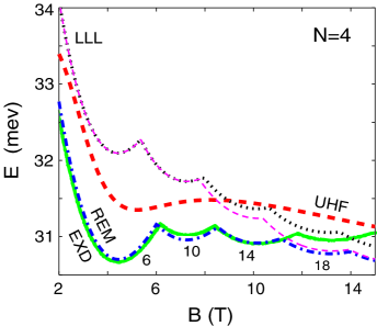
Figure 1: (Color online) Two-step-method versus EXD calculations: Ground-state energies for $N=4$ electrons (referenced to $4\hbar\Omega$) as a function of the magnetic field $B$. Thick dashed line (red): broken-symmetry UHF (SEM). Solid line (green): EXD (from Ref. ruan2, ). Thick dashed-dotted line (blue): REM. Thin dashed line (violet, marked LLL): the commonly used approximate energies $\widetilde{E}^{\text{EXD}}_{\text{tot,LLL}}(B)$ [see Eq. (13)]. Thin dotted line (black): $\widetilde{E}^{\text{REM}}_{\text{tot,LLL}}(B)$ (see section II.B). For $B<8$ T, the $\widetilde{E}^{\text{EXD}}_{\text{tot,LLL}}(B)$ and $\widetilde{E}^{\text{REM}}_{\text{tot,LLL}}(B)$ curves coincide; we have checked that these curves approach each other also at larger values of $B$, outside the plotted range. Numbers near the bottom curves denote the value of magic angular momenta [$L_{m}$, see Eq. (3)] of the ground state. Corresponding fractional filling factors are specified by $\nu=N(N-1)/(2L_{m})$. Parameters used: confinement $\hbar\omega_{0}=3.60$ meV, dielectric constant $\kappa=13.1$, effective mass $m^{*}=0.067m_{e}$.

III Comparison of approximate results with exact diagonalization calculations

III.1 Ground-state energies in external confinement

Before proceeding with the presentation of results for $N>10$, we demonstrate the accuracy of the two-step method through comparisons with existing EXD results for smaller sizes. In Fig. 1, our calculations for ground-state energies as a function of $B$ are compared to EXD calculations ruan2 for $N=4$ electrons in an external parabolic confinement. The thick dotted line (red) represents the broken-symmetry UHF approximation (first step of our method), which naturally is a smooth curve lying above the EXD one [solid line (green)]. The results obtained after restoration of symmetry [dashed-dotted line (blue); marked as REM] agree very well with the EXD one in the whole range 2 T$<B<$ 15 T. note1 We recall here that, for the parameters of the QD, the electrons form in the intrinsic frame of reference a square about the origin of the dot, i.e., a (0,4) configuration, with the zero indicating that no electron is located at the center. According to Eq. (3), $L_{0}=6$, and the magic angular momenta are given by $L_{m}=6+4k$, $k=0$, 1, 2, …

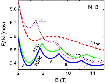
Figure 2: (Color online) Two-step method versus EXD calculations: Ground-state energies (per particle, referenced to $\hbar\Omega$) for $N=3$ electrons. The electrons are arranged in a (0,3) structure in the intrinsic frame of reference. Thick dashed line (red): broken-symmetry UHF (SEM). Thinner solid line (green): EXD (from Ref. haw1, ). Thick solid line (blue): REM. Thin dashed line (violet): the commonly used approximate energies $\widetilde{E}^{\text{EXD}}_{\text{tot,LLL}}(B)$ (see text). Thin dotted line (black): $\widetilde{E}^{\text{REM}}_{\text{tot,LLL}}(B)$ (see text). For $B<8$ T, the $\widetilde{E}^{\text{EXD}}_{\text{tot,LLL}}(B)$ and $\widetilde{E}^{\text{REM}}_{\text{tot,LLL}}(B)$ curves coincide; we have checked that these curves approach each other also at larger values of $B$, outside the plotted range. Numbers denote the value of magic angular momenta ($L_{m}$) of the ground state. Corresponding fractional filling factors are specified by $\nu=N(N-1)/(2L_{m})$. Parameters used: confinement $\hbar\omega_{0}=3.37$ meV, dielectric constant $\kappa=12.4$, effective mass $m^{*}=0.067m_{e}$.

To further evaluate the accuracy of the two-step method, we also display in Fig. 1 [thin dashed line (violet)] ground-state energies calculated with the commonly used maks ; yang ; jeon approximation $\widetilde{E}^{\text{EXD}}_{\text{tot,LLL}}(B)$ (see section II.B). We find that the energies $\widetilde{E}^{\text{EXD}}_{\text{tot,LLL}}(B)$ tend to substantially overestimate the REM (and EXD) energies for lower values of $B$ (e.g., by as much as 5.5% at $B\sim 4$ T). On the other hand, for higher values of $B$ ($>$ 12 T), the energies $\widetilde{E}^{\text{EXD}}_{\text{tot,LLL}}(B)$ tend to agree rather well with the REM ones. A similar behavior is exhibited also by the $\widetilde{E}^{\text{REM}}_{\text{tot,LLL}}(B)$ energies [the interaction energies are calculated within the LLL using the REM wave function; dotted line (black)]. We have found that the overestimation exhibited by the $\widetilde{E}^{\text{EXD}}_{\text{tot,LLL}}(B)$ energies is due to the fact that the actual dimensionless Coulomb coefficient $\widetilde{{\cal E}}^{\text{EXD}}_{\text{int,LLL}}(L)$ [See Eq. (13)] is not independent of the magnetic field, but decreases slowly as $B$ decreases when the effect of the confinement is considered (see Appendix B). A similar agreement between REM and EXD results, and a similar inaccurate behavior of the limiting-case approximation, was found by us also for $N=3$ electrons in the range 2 T $<B<$ 16 T shown in Fig. 2 (the EXD calculation was taken from Ref. haw1, ).

In all cases, the total energy of the REM is lower than that of the SEM (see, e.g., Figs. 1 and 2). Indeed, a theorem discussed in Sec. III of Ref. low, , pertaining to the energies of projected wave functions, guarantees that this lowering of energy applies for all values of $N$ and $B$.

III.2 Yrast rotational band at $B\rightarrow\infty$

As a second accuracy test, we compare in Table I REM and EXD results for the interaction energies of the yrast band for $N=6$ electrons in the lowest Landau level [an yrast state is the lowest energy state for a given magic angular momentum $L_{m}$, Eq. (3)]. The relative error is smaller than 0.3%, and it decreases steadily for larger $L$ values.

Table 1: Comparison of yrast-band energies obtained from REM and EXD calculations for $N=6$ electrons in the lowest Landau level, that is in the limit $B\rightarrow\infty$. In this limit the external confinement can be neglected and only the interaction energy contributes to the yrast-band energies. Energies in units of $e^{2}/(\kappa l_{B})$. For the REM results, the (1,5) polygonal-ring arrangement was considered. For $L<140$, see Table IV in Ref. yl, (b) and Table III in Ref. yl2, (c). The values of the fractional filling may be obtained for each $L$ as $\nu=N(N-1)/(2L)$.

$L$	REM	EXD	Error (%)
140	1.6059	1.6006	0.33
145	1.5773	1.5724	0.31
150	1.5502	1.5455	0.30
155	1.5244	1.5200	0.29
160	1.4999	1.4957	0.28
165	1.4765	1.4726	0.27
170	1.4542	1.4505	0.26
175	1.4329	1.4293	0.25
180	1.4125	1.4091	0.24
185	1.3929	1.3897	0.23
190	1.3741	1.3710	0.23
195	1.3561	1.3531	0.22
200	1.3388	1.3359	0.21

IV Illustrative examples from microscopic REM calculations

IV.1 Which ring isomer has the lowest ground-state energy?: REM versus UHF energies

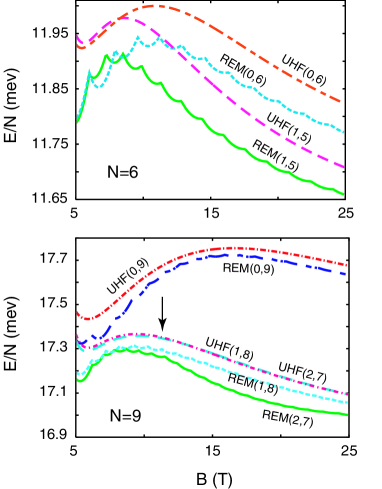
Figure 3: (Color online) Comparison of REM and UHF ground-state energies per particle (referenced to $\hbar\Omega$) associated with different ring isomers for $N=6$ and $N=9$ electrons as a function of the magnetic field $B$. The curves are labeled with the computational method and the isomer $(n_{1},n_{2})$. To the left of the vertical arrow (at $B=11.5$ T), the UHF(1,8) curve is energetically favored. To the right of the vertical arrow, the UHF(2,7) curve is energetically favored. Parameters used: confinement $\hbar\omega_{0}=3.60$ meV, dielectric constant $\kappa=13.1$, effective mass $m^{*}=0.067m_{e}$.

For a given number $N$ of electrons, there existkon in general more than one polygonal-ring isomers, associated with stable and metastable equilibrium configurations of $N$ electrons inside an external harmonic confinemnet $\hbar\omega_{0}$. Figure 3 displays UHF and REM ground-state energies for $N=6$ and $N=9$ electrons associated with the various classical polygonal-ring configurations. For $N=6$, one has two isomers, i.e., a (0,6) configuration and a (1,5) configuration (with one lectron at the center). For $N=9$ electrons, there exist three different isomers, i.e., (0,9), (1,8), and (2,7). From the bottom panel in Fig. 3, we observe that for $N=9$ electrons, the lowest REM energies correspond to the classically stable isomer, i.e., to the (2,7) configuration with two electrons in the inner ring and seven electrons in the outer ring. In particular, we note that the (0,9) isomer (which may be associated with a single-vortex state) yileds REM energies far above the (2,7) one in the whole magnetic-field range 5 T $<B<$ 25 T, and in particular for magnetic fields immediately above those associated with the MDD (the so-called MDD break-up range); the MDD for $N=9$ electrons has an angular momentum $L_{0}=36$ and corresponds to the first energy oscillation in the figure.

We have found that the $(0,N)$ isomer is not associated with REM ground energies for any magnetic-field range in all cases with $N\geq 7$. The only instance when the $(0,N)$ configuration is associated with a REM ground-state energy is the $N=6$ case [see Fig. 3, top frame], where the REM energy of the (0,6) configuration provides the ground-state energy in the range 6.1 T $<B<$ 7.7 T, immediately after the break-up of the MDD.

For comparison, we have also plotted in Fig. 3 the UHF energies as a function of the magnetic field. Most noticeable is the fact that the REM ground states, compared to the UHF ones, may result in a different ordering of the isomers. For example, in the range 5 T $<B<$ 6.1 T, the UHF indicates, by a small energetic advantage, the (0,6) as the ground-state configuration associated with the MDD, while the REM specifies the (1,5) arrangement as the ground-state configuration. A similar switching of the ground-state isomers is also seen between the (1,8) and (2,7) configurations in the case of $N=9$ electrons in the magnetic-field range 5 T $<B<$ 11.5 T. We conclude that transitions between the different electron-molecule isomers derived from UHF energies aloneszaf ; note32 are not reliable.

IV.2 The case of $N=9$ electrons

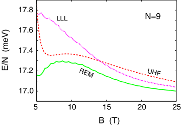
Figure 4: (Color online) Ground-state energies [i.e., for the (2,7) configuration] for $N=9$ electrons (per particle, referenced to $\hbar\Omega$) as a function of the magnetic field $B$. Dashed line (red): UHF (SEM). Solid line (blue): REM. Dotted line (black): approximate energies $\widetilde{E}^{\text{REM}}_{\text{tot,LLL}}(B)$ (see text). Parameters used: confinement $\hbar\omega_{0}=3.60$ meV, dielectric constant $\kappa=13.1$, effective mass $m^{*}=0.067m_{e}$.

In figure 4 we show ground-state energies for the case of $N=9$ electrons, which have a nontrivial double-ring configuration $(n_{1},n_{2})$. Here, the most stable configuration for classical point chargeskon is $(2,7)$, for which we have carried UHF (SEM) and REM (projected) calculations in the magnetic field range 5 T $<B<$ 25 T. We also display in Fig. 4 the energies $\widetilde{E}^{\text{REM}}_{\text{tot,LLL}}(B)$ [dotted curve (black)], which, as in the $N=4$ and $N=3$ cases discussed in the section III, overestimate the ground-state energies, in particular for smaller $B$. note39 In keeping with the findings for smaller sizes yl ^(c) [with $(0,N)$ or $(1,N-1)$ configurations], both the UHF and the REM ground-state energies of the $N=9$ case approach as $B\rightarrow\infty$ the classical equilibrium energy of the (2,7) polygonal configuration [i.e., 16.75 meV; 4.088$E_{0}$ in the units of Ref. kon, , $E_{0}\equiv(m^{*}\omega_{0}^{2}e^{4}/2\kappa^{2})^{1/3}$].

In analogy with smaller sizes [see, e.g., Figs. 1 and 2 for $N=4$ and $N=3$], the REM ground-state energies in Fig. 4 exhibit oscillations as a function of $B$. These oscillations reflect the incompressibility of the many-body states associated with magic angular momenta. The magic angular momenta are specified by the number of electrons on each ring, and in general they are given by $L_{m}=N(N-1)/2+\sum_{q=1}^{r}k_{q}n_{q}$, where the $n_{q}$’s are the number of electrons located in the $q$th ring and the $k_{q}$’s are non-negative integers; in particular, $L_{m}=36+2k_{1}+7k_{2}$ for the $N=9$ case in Fig. 4. An analysis of the actual values taken by the set of indices $\{k_{1},k_{2}\}$ reveals several additional trends that further limit the allowed values of ground-state $L_{m}$’s. In particular, starting with the values $\{k_{1}=0,k_{2}=0\}$ at $B=5$ T ($L_{m}^{\text{MDD}}=36$), the indices $\{k_{1},k_{2}\}$ reach the values $\{2,24\}$ at $B=25$ T ($L_{m}=208$). As seen form Table II, the outer index $k_{2}$ has a short period, while the inner index $k_{1}$ exhibits a longer period and increases much more slowly than $k_{2}$. This behavior minimizes the total kinetic energy of the independently rotating rings (having a variable radius, see section V below).

Table 2: Ground-state magic angular momenta and their decomposition $\{k_{1},k_{2}\}$ for $N=9$ in the nagnetic-field range 5 T $\leq B\leq$ 25 T. These results correspond to the REM [see lower curve in Fig. 4, with the electrons arranged in a (2,7) structure]. The parameters used are as in Fig. 4.

$L_{m}$	$k_{1}$	$k_{2}$	$L_{m}$	$k_{1}$	$k_{2}$
36	0	0	129	1	13
43	0	1	136	1	14
50	0	2	143	1	15
57	0	3	150	1	16
64	0	4	157	1	17
71	0	5	164	1	18
78	0	6	171	1	19
87	1	7	173	2	19
94	1	8	180	2	20
101	1	9	187	2	21
108	1	10	194	2	22
115	1	11	201	2	23
122	1	12	208	2	24

Table 3: Ground-state magic angular momenta and their decomposition $\{k_{1},k_{2}\}$ for $N=9$ electrons associated with the $\widetilde{E}_{\text{tot,LLL}}^{\text{REM}}$ curve [top curve in Fig. 4; see section II.B for an explanation of notation; the electrons are arranged in a (2,7) structure].

$L_{m}$	$k_{1}$	$k_{2}$	$L_{m}$	$k_{1}$	$k_{2}$
36	0	0	57	0	3
45	1	1	64	0	4
52	1	2	71	0	5

We also list in Table III the first few pairs of indices $\{k_{1},k_{2}\}$ associated with the $\widetilde{E}_{\text{tot,LLL}}^{\text{REM}}$ curve (see top dotted curve in Fig. 4). It can be seen that the magic angular momenta are different from those associated with the REM curve, when the confinement is taken into consideration using the full projected wave function in Eq. (2). The magic angular momenta of the $\widetilde{E}_{\text{tot,LLL}}^{\text{REM}}$ curve coincide with the $L_{m}$’s of the EXD within the LLL, and thus are characterized by having $L_{0}+N=45$ (instead of $L_{0}+n_{2}=43$) as the magic angular momentum immediately following that of the MDD (i.e., $L_{0}=36$). The $L_{0}+N$ magic angular momentum is associated with the $(0,N)$ ring arrangement, which can be interpreted as a single “vortex-in-the-center” state.

Based on EXD calculations restricted to the lowest Landau level yang2 ; nie ; reim (that is, $\widetilde{E}_{\text{int,LLL}}^{\text{EXD}}$ or $\widetilde{E}_{\text{tot,LLL}}^{\text{EXD}}$ in our notation), it has been conjectured that for QDs with $N<15$, the break-up of the MDD with increasing $B$ proceeds through the formation of the above mentioned single central vortex state. However, our REM calculations show (see also the case of $N=11$ electrons in section IV.C and the case of $N=17$ electrons in section IV.D) that taking into account properly the influence of the confinement does not support such a scenario. Instead, the break-up of the MDD resembles an edge reconstruction and it proceeds (for all dots with $N>6$) through the gradual detachement of the outer ring associated with the classical ground-state polygonal configuration (see Table II for the case of $N=9$ electrons). The only case we found where the break-up of the MDD proceeds via a (0,N) vortex state is the one with $N=6$ electrons (see section IV.A),; and naturally the cases with $N\leq 5$.

Figure 5: (Color online) REM radial electron densities for the MDD ($L_{m}=L_{0}=36$) of $N=9$ electrons [in the (2,7) ground-state configuration] at (a) $B\rightarrow\infty$, i.e., in the lowest Landau level and (b) at $B=5.5$ T. Parameters used in (b): confinement $\hbar\omega_{0}=3.60$ meV, dielectric constant $\kappa=13.1$, effective mass $m^{*}=0.067m_{e}$. Lengths: (a) in units of the magnetic length $l_{B}$; (b) in units of $R_{0}=(2e^{2}/m^{*}\kappa\omega_{0}^{2})^{1/3}$. Electron densities: (a) in units of $1/l_{B}^{2}$; (b) in units of $1/R_{0}^{2}$. Normalization: $2\pi\int_{0}^{\infty}\rho(r)rdr=N$.

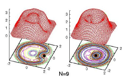
Figure 6: (Color online) Conditional probability distributions obtained from REM wave functions of the MDD ($L_{0}=36$) for $N=9$ electrons at $B=5.5$ T [see Fig. 5(b)]. The electrons are arranged in a (2,7) structure. The observation point is denoted by a solid dot. On the left, the observation point is located on the outer shell, and on the right it is located on the inner shell. Parameters used: confinement $\hbar\omega_{0}=3.60$ meV, dielectric constant $\kappa=13.1$, effective mass $m^{*}=0.067m_{e}$. Lengths in units of $R_{0}=(2e^{2}/(\kappa m^{*}\omega_{0}^{2}))^{1/3}$. CPDs (vertical axes) in arbitrary units.

As another illustration of the subtle, but important, differences that exist between wave functions defined exclusively within the LLL and those specified by the REM wave function for finite $B$ in Eq. (2), we display in Fig. 5 for $N=9$ electrons the radial electron densities of the MDD at $B\rightarrow\infty$ and at $B=5.5$ T. While the electron density of the MDD in the LLL ($B\rightarrow\infty$) is constant in the central region [up to $r\approx 3l_{B}$, see Fig. 5(a)], the corresponding density at $B=5.5$ T displays the characteristic oscillation corresponding to the (2,7) multi-ring structure [see Fig. 5(b)]; the latter behavior is due to the mixing of higher Landau levels. To further illustrate the (2,7) crystalline character of the MDD when higher Landau levels are considered, we display in Fig. 6 the corresponding CPDs associated with the REM wave function of the MDD at $B=5.5$ T and an external confinement of $\hbar\omega_{0}=3.6$ meV. Our conclusions concerning the MDD electron densities (and CPDs) are supported by EXD calculations for $N=4$ electrons.note47 Note that, while the ring structure is well developed in the CPDs shown in Fig. 6, the internal (2,7) structure of the rings (see in particular the outer ring in the left panel in Fig. 6) is rather weak, as expected for the lowest angular momentum $L_{0}$ (MDD). However, the ring structure is easily discernible in contrast to the CPDs for the MDD restricted to the LLL where structureless CPDs (as well as structureless electron densities) are found.

IV.3 The case of $N=11$ electrons

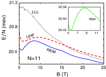
Figure 7: (Color online) Ground-state energies for $N=11$ electrons (per particle, referenced to $\hbar\Omega$) as a function of the magnetic field $B$. Dashed line (red): UHF (SEM). Solid line (blue): REM. Dotted line (black): Approximate energies $\widetilde{E}^{\text{REM}}_{\text{tot,LLL}}(B)$ (see text). Parameters used: confinement $\hbar\omega_{0}=3.60$ meV, dielectric constant $\kappa=13.1$, effective mass $m^{*}=0.067m_{e}$. The inset shows a magnification of the REM curve in the range 5 T $<B<$ 12 T.

Table 4: Ground-state magic angular momenta and their decomposition $\{k_{1},k_{2}\}$ for $N=11$ in the nagnetic-field range 5 T $\leq B\leq$ 25 T. The results correspond to the REM (see lower curve in Fig. 7). The parameters used are as in Fig. 7.

$L_{m}$	$k_{1}$	$k_{2}$	$L_{m}$	$k_{1}$	$k_{2}$
55	0	0	165	2	13
63	0	1	173	2	14
71	0	2	181	2	15
79	0	3	189	2	16
90	1	4	197	2	17
98	1	5	205	2	18
106	1	6	213	2	19
114	1	7	224	3	20
122	1	8	232	3	21
130	1	9	240	3	22
138	1	10	248	3	23
146	1	11	256	3	24
154	1	12

Figure 7 presents the case for the ground-state energies of a QD with $N=11$ electrons, which have a nontrivial double-ring configuration $(n_{1},n_{2})$. The most stablekon classical configuration is $(3,8)$, for which we have carried UHF (SEM) and REM (projected) calculations in the magnetic field range 5 T $<B<$ 25 T. Figure 7 also displays the LLL ground-state energies $\widetilde{E}^{\text{REM}}_{\text{tot,LLL}}(B)$ [dotted curve (black)], which, as in previous cases, overestimate the ground-state energies for smaller $B$. The approximation $\widetilde{E}^{\text{REM}}_{\text{tot,LLL}}(B)$, however, can be used to calculate ground-state energies for higher values of $B$. In keeping with the findings for smaller sizes yl ^(c) [with $(0,N)$ or $(1,N-1)$ configurations], we found that both the UHF and the REM ground-state energies approach, as $B\rightarrow\infty$, the classical equilibrium energy of the (3,8) polygonal configuration [i.e., 19.94 meV; 4.865$E_{0}$ in the units of Ref. kon, , $E_{0}\equiv(m^{*}\omega_{0}^{2}e^{4}/2\kappa^{2})^{1/3}$].

In analogy with smaller sizes [see, e.g., Figs. 1, 2, and 4 for $N=4$, 3, and 9, respectively], the REM ground-state energies in Fig. 7 exhibit oscillations as a function of $B$ (see in particular the inset). As discussed in section IV.B, these oscillations are associated with magic angular momenta, specified by the number of electrons on each ring. For $N=11$ they are given by Eq. (3), i.e., $L_{m}=55+3k_{1}+8k_{2}$, with the $k_{q}$’s being nonnegative integers. As was the case with $N=9$ electrons, an analysis of the actual values taken by the set of indices $\{k_{1},k_{2}\}$ reveals several additional trends that further limit the allowed values of ground-state $L_{m}$’s. In particular, starting with the values $\{0,0\}$ at $B=5$ T ($L_{0}=55$), the indices $\{k_{1},k_{2}\}$ reach the values $\{3,24\}$ at $B=25$ T ($L_{m}=256$). As seen from Table IV, the outer index $k_{2}$ changes faster than the inner index $k_{1}$. This behavior minimizes the total kinetic energy of the independently rotating rings; indeed, the kinetic energy of the inner ring (as a function of $k_{1}$) rises faster than that of the outer ring (as a function of $k_{2}$) due to smaller moment of inertia (smaller radius) of the inner ring [see Eq. (14)].

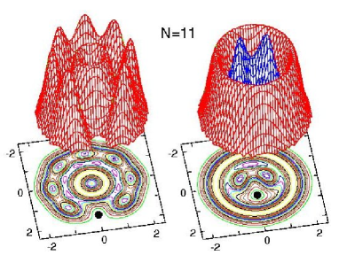
Figure 8: (Color online) REM conditional probability distributions for $N=11$ electrons at $B=10$ T ($L=106$). The electrons are arranged in a (3,8) structure. The observation point (solid dot) is placed on (left) the outer ring at $r_{0}=1.480R_{0}$, and (right) on the inner ring at $r_{0}=0.557R_{0}$. Parameters used: confinement $\hbar\omega_{0}=3.60$ meV, dielectric constant $\kappa=13.1$, effective mass $m^{*}=0.067m_{e}$. Lengths in units of $R_{0}=(2e^{2}/m^{*}\kappa\omega_{0}^{2})^{1/3}$. CPDs (vertical axes) in arbitrary units.

In addition to the overestimation of the ground-state energy values, particularly for smaller magnetic fields (see Fig. 7 and our above discussion), the shortcomings of the LLL approximation pertaining to the ground-state ring configurations [see section II.B, Eq. (13)], as discussed by us above for $N=9$, persist also for $N=11$. In particular, we find that according to the LLL approximation the ground-state angular-momentum immediately after the MDD ($L_{0}=55$) is $L_{m}=66$, i.e., the one associated with the $(0,N)$ vortex-in-the-center configuration. This result, erroneously stated in Ref. reim, as the ground state, disagrees with the correct result that includes the effect of the confinement – listed in Table IV, where the ground-state angular momentum immediately following the MDD is $L_{m}=63$. This angular momentum corresponds to the classicaly most stable (3,8) ring configuration – that is a configuration with no vortex at all.

Figure 8 displays the REM conditional probability distributions for the ground state of $N=11$ electrons at $B=10$ T ($L_{m}=106$). The (3,8) ring configuration is clearly visible. We note that when the observation point is placed on the outer ring (left panel), the CPD reveals the crystalline structure of this ring only; the inner ring appears to have a uniform density. To reveal the crystalline structure of the inner ring, the observation point must be placed on this ring; then the outer ring appears to be uniform in density. This behavior suggests that the two rings rotate independently of each other, a property that we will explore in section V to derive an approximate expression for the yrast rotational spectra associated with an arbitrary number of electrons.

IV.4 The case of $N=17$ electrons

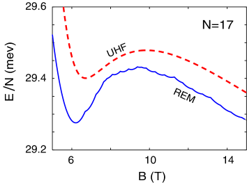
Figure 9: (Color online) Ground-state energies (per particle, referenced to $\hbar\Omega$) for $N=17$ electrons as a function of the magnetic field $B$. The electrons are arranged in a (1,6,10) structure. Dashed line (red): UHF. Solid line (blue): REM. Parameters used: confinement $\hbar\omega_{0}=3.6$ meV, dielectric constant $\kappa=13.1$, effective mass $m^{*}=0.067m_{e}$.

Figure 9 presents (for 5 T $\leq B\leq$ 15 T) REM and UHF ground-state energies for $N=17$ electrons, which have a (1,6,10) three-ring configuration as the most stable classical arrangement. kon

In analogy with smaller sizes [see, e.g., previous figures for $N\leq 12$] the REM ground-state energies in Fig. 9 exhibit oscillations as a function of $B$, and each oscillation is associated with a given particular (magic) value of the angular momentum. Earlier in this section we discussed the physical origins of the magic angular momenta. As before, the magic angular momenta are specified by the number of electrons on each ring [(3)], with $L_{0}=136$ and $L_{m}=136+6k_{2}+10k_{3}$ for $N=17$; $k_{q}$’s being non-negative integers (the central electron does not contribute to the total angular momentum). Analysis of the particular values taken by the set of indices $\{k_{2},k_{3}\}$ reveals similar trends to those found for the cases with $N=9$ and $N=11$ electrons. In particular, starting with the values $\{0,0\}$ at $B=5$ T ($L_{0}=136$), the indices $\{k_{2},k_{3}\}$ reach the values $\{k_{2}=5,k_{3}=18\}$ at $B=15$ T ($L_{m}=346$). As seen from Table V, the outer index $k_{3}$ changes faster, than the inner index $k_{2}$. This behavior minimizes the total kinetic energy of the independently rotating rings, as was already discussed for $N=9$ and $N=11$ electrons.

We have also calculated the ground-state energies for $N=17$ electrons in the LLL approximation, i.e., we calculated the quantity $\widetilde{E}^{\text{REM}}_{\text{tot,LLL}}(B)$ (not shown in Fig. 9). We find once more that $\widetilde{E}^{\text{REM}}_{\text{tot,LLL}}(B)$ overestimates the ground-state energies in the magnetic-field range covering the MDD and the range immediately above the MDD. For $N=17$, however, the shortcoming of the LLL approximation is not reflected in the determination of the ground-state ring configurations. We find that for $N=17$ the LLL approximation yields a (1,6,10) ring configuration (with $L_{m}=146$) for the ground state immediately following the MDD, in agreement with the REM configurations listed in Table V.

Table 5: Ground-state magic angular momenta and their decomposition $\{k_{2},k_{3}\}$ for $N=17$ electrons in the nagnetic-field range 5 T $\leq B\leq$ 15 T. The rersults correspond to the REM (see lower curve in Fig. 9). The parameters used are as in Fig. 9.

$L_{m}$	$k_{2}$	$k_{3}$	$L_{m}$	$k_{2}$	$k_{3}$
136	0	0	238	2	9
146	0	1	248	2	10
156	0	2	264	3	11
166	0	3	274	3	12
172	1	3	284	3	13
182	1	4	294	3	14
192	1	5	310	4	15
202	1	6	320	4	16
212	1	7	330	4	17
218	2	7	340	4	18
228	2	8	346	5	18

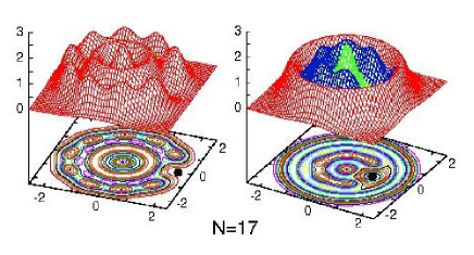
Figure 10: (Color online) Grond-state conditional probability distributions, CPDs, obtained from REM wave functions for the ground state of $N=17$ electrons at $B=10$ T ($L=228$). The electrons are arranged in a (1,6,10) structure. The observation point (solid dot) is placed on the outer ring at $r_{0}=1.858R_{0}$ (left frame), and on the inner ring at $r_{0}=0.969R_{0}$ (right frame). The rest of the parameters are the same as in Fig. 9. Lengths in units of $R_{0}=(2e^{2}/(\kappa m^{*}\omega_{0}^{2}))^{1/3}$. CPDs (vertical axes) in arbitrary units.

V REM YRAST BAND EXCITATION SPECTRA AND DERIVATION OF ANALYTIC APPROXIMATE FORMULA

In Fig. 10, we display the CPD for the REM wave function of $N=17$ electrons. This case has a nontrivial three-ring structure (1,6,10), kon which is sufficiently complex to allow generalizations for larger numbers of particles. The remarkable combined character (partly crystalline and partly fluid leading to a non-classical rotational inertia, see section VI) of the REM is illustrated in the CPDs of Fig. 10. Indeed, as the two CPDs [reflecting the choice of taking the observation point [${\bf r}_{0}$ in Eq. (8)] on the outer (left frame) or the inner ring (right frame)] reveal, the polygonal electron rings rotate independently of each other. Thus, e.g., to an observer located on the inner ring, the outer ring will appear as having a uniform density, and vice versa. The wave functions obtained from exact diagonalization exhibit also the property of independently rotating rings [see e.g., the $N=12$ and $L=132$ ($\nu=1/2$) case in Fig. 11], which is a testimony to the ability of the REM wave function to capture the essential physics jain of a finite number of electrons in high $B$. In particular, the conditional probability distribution obtained for exact diagonalization wave functions in Fig. 11 exhibits the characteristics expected from the CPD evaluated using REM wave functions for the (3,9) configuration and with an angular-momentum decomposition into shell contributions [see Eqs. (2) and (4)] $L_{1}=3+3k_{1}$ and $L_{2}=63+9k_{2}$ ($L_{1}+L_{2}=L_{m}$; for $L_{m}=132$ the angular-momentum decomposition is $L_{1}=6$ and $L_{2}=126$).

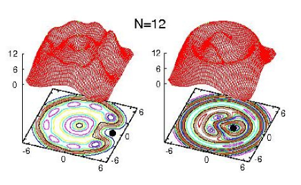
Figure 11: (Color online) CPDs for $N=12$ electrons and with angular momentum $L=132$ ($\nu=1/2$) calculated with EXD in the lowest Landau level. The electrons are arranged in a (3,9) structure. The observation point (solid dot) is placed on the outer ring at $r_{0}=5.22l_{B}$ (left frame), and on the inner ring at $r_{0}=1.87l_{B}$ (right frame). Lengths in units of $l_{B}$. CPDs (vertical axes) in arbitrary units.

In addition to the conditional probabilities, the solid/fluid character of the REM is revealed in its excited rotational spectrum for a given $B$. From our microscopic calculations based on the wave function in Eq. (2), we have derived (see below) an approximate (denoted as “app”), but analytic and parameter-free, expression [see Eq. (19) below] which reflects directly the nonrigid (nonclassical) character of the REM for arbitrary size. This expression allows calculation of the energies of REMs for arbitrary $N$, given the corresponding equilibrium configuration of confined classical point charges.

We focus on the description of the yrast band at a given $B$. Motivated by the aforementioned nonrigid character of the rotating electron molecule, we consider the following kinetic-energy term corresponding to a $(n_{1},...,n_{q},...,n_{r})$ configuration (with $\sum_{q=1}^{r}n_{q}=N$):

$$E_{\text{app}}^{\text{kin}}(N)=\sum_{q=1}^{r}\hbar^{2}L_{q}^{2}/(2{\cal J}_{q}(a_{q}))-\hbar\omega_{c}L/2,$$ (14)

where $L_{q}$ is the partial angular momentum associated with the $q$th ring about the center of the dot and the total angular momentum is $L=\sum_{q=1}^{r}L_{q}$. ${\cal J}_{q}(a_{q}))\equiv n_{q}m^{*}a_{q}^{2}$ is the rotational moment of inertia of each individual ring, i.e., the moment of inertia of $n_{q}$ classical point charges on the $q$th polygonal ring of radius $a_{q}$. To obtain the total energy, $E_{L}^{\text{REM}}$, we include also the term $E_{\text{app}}^{\text{hc}}(N)=\sum_{q=1}^{r}{\cal J}_{q}(a_{q})\Omega^{2}/2$ due to the effective harmonic confinement $\Omega$ [see discussion of Eq. (1)], as well as the interaction energy $E_{\text{app}}^{C}$,

$$E_{\text{app}}^{C}(N)=\sum_{q=1}^{r}\frac{n_{q}S_{q}}{4}\frac{e^{2}}{\kappa a_{q}}+\sum_{q=1}^{r-1}\sum_{s>q}^{r}V_{C}(a_{q},a_{s}).$$ (15)

The first term is the intra-ring Coulomb-repulsion energy of $n_{q}$ point-like electrons on a given ring, with a structure factor

$$S_{q}=\sum_{j=2}^{n_{q}}(\sin[(j-1)\pi/n_{q}])^{-1}.$$ (16)

The second term is the inter-ring Coulomb-repulsion energy between rings of uniform charge distribution corresponding to the specified numbers of electrons on the polygonal rings. The expression fo $V_{C}$ is

$$V_{C}(a_{q},a_{s}) = n_{q}{n_{s}}\;{{}_{2}F_{1}}[3/4,1/4;1;4a_{q}^{2}a_{s}^{2}(a_{q}^{2}+a_{s}^{2})^{-2}]$$ (17)

$$\times e^{2}(a_{q}^{2}+a_{s}^{2})^{-1/2}/\kappa,$$

where ${{}_{2}F_{1}}$ is the hypergeometric function.

For large $L$ (and/or $B$), the radii of the rings of the rotating molecule can be found by neglecting the interaction term in the total approximate energy, thus minimizing only $E_{\text{app}}^{\text{kin}}(N)+E_{\text{app}}^{\text{hc}}(N)$. One finds

$$a_{q}=\lambda\sqrt{L_{q}/n_{q}};$$ (18)

i.e., the ring radii depend on the partial angular momentum $L_{q}$, reflecting the lack of radial rigidity. Substitution into the above expressions for $E_{\text{app}}^{\text{kin}}$, $E_{\text{app}}^{\text{hc}}$, and $E_{\text{app}}^{C}$ yields for the total approximate energy the final expression:

$$E_{\text{app},L}^{\text{REM}} (N)=\hbar(\Omega-\omega_{c}/2)L+$$ (19)

$$\sum_{q=1}^{r}\frac{C_{V,q}}{L_{q}^{1/2}}+\sum_{q=1}^{r-1}\sum_{s>q}^{r}V_{C}(\lambda\sqrt{\frac{L_{q}}{n_{q}}},\lambda\sqrt{\frac{L_{s}}{n_{s}}}),$$

where the constants

$$C_{V,q}=0.25n_{q}^{3/2}S_{q}e^{2}/(\kappa\lambda).$$ (20)

For simpler $(0,N)$ and $(1,N-1)$ ring configurations, Eq. (19) reduces to the expressions reported earlier.^7(c), mak

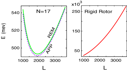
Figure 12: (Color online) Left: Yrast spectrum for $N=17$ electrons at a high magnetic field $B=100$ T. Approximate analytic expression [Eq. (19), dashed line (violet)] compared with microscopic REM calculations [Eq. (5), solid line (green)]. Right: The corresponding classical (rigid rotor) energy $E^{\text{rig}}_{L}$ for $N=17$ electrons (see text). The microscopic REM energies are referenced relative to the zero-point energy, $17\hbar\Omega$. Energies were calculated for magic angular momenta $L=L_{1}+L_{2}+L_{3}$ with $L_{1}=0$, $L_{2}=21+6k_{2}$ and $k_{2}=30$, and $L_{3}=115+10k_{3}$. The parameters are the same as in Fig. 9. Note the much larger energy scale for the classical case (right frame), leading to a non-rigidity index for the REM of $\alpha\sim 0.99$ (see text).

VI A non-rigid crystalline phase: Non-classical rotational inertia of electrons in quantum dots

In Fig. 12 (left frame), and for a sufficiently high magnetic field (e.g., $B=100$ T such that the Hilbert space of the system reduces to the lowest Landau level), we compare the approximate analytic energies $E_{\text{app},L}^{\text{REM}}$ with the microscopic energies $E_{L}^{\text{REM}}$ calculated from Eq. (5) using the same parameters as in Fig. 9 for $N=17$ electrons. The two calculations agree well, with a typical difference of less than 0.5% between them. More important is the marked difference between these results and the total energies of the classical (rigid rotor) molecule ($E^{\text{rig}}_{L}$), plotted in the right frame of Fig. 12; the latter are given by

$$E^{\text{rig}}_{L} = \hbar^{2}L^{2}/(2{\cal J}_{\text{rig}})+0.5\sum_{i=1}^{N}m^{*}\omega_{0}^{2}|Z_{i}|^{2}+$$ (21)

$$\sum_{i=1}^{N}\sum_{j>i}^{N}e^{2}/(\kappa|Z_{i}-Z_{j}|),$$

with the rigid moment of inertia being note3

$${\cal J}_{\text{rig}}=\sum_{i=1}^{N}m^{*}|Z_{i}|^{2}.$$ (22)

The disagreement between the REM and the classical energies is twofold: (i) The $L$ dependence is different, and (ii) The REM energies are three orders of magnitude smaller than the classical ones. That is, the energy cost for the rotation of the REM is drastically smaller than for the classical rotation, thus exhibiting non-classical rotational behavior. In analogy with Ref. legg, , we define a “non-rigidity” index

$$\alpha=(E^{\text{rig}}_{L}-E_{L}^{\text{REM}})/E^{\text{rig}}_{L}.$$ (23)

For the case displayed in Fig. 12, we find that this index varies (for $1116\leq L\leq 3716$) from $\alpha=0.978$ to $\alpha=0.998$, indicating that the rotating electron molecule, while possessing crystalline correlations is (rotationally) of a high non-rigid nature. We remark that our definition of $\alpha$ in Eq. (23) was motivated by a similar form of an index of supefluid fraction introduced in Ref. legg, ; we do not mean to imply the presence of a superfluid component for electrons in quantum dots.

In the context of the appearance of supersolid behavior of ⁴He under appropriate conditions, formation of a supersolid fraction is often discussed in conjunction with the presence of (i) real defects and (ii) real vacancies. anlf ; ches Our REM wave function [Eq. 2] belongs to a third possibility, namely to virtual defects and vacancies, with the number of particles equal to the number of lattice sites (in the context of ⁴He, the possibility of a supersolid with equal number of particles and lattice sites is mentioned in Ref. legg2, ). Indeed, the azimuthal shift of the electrons by $(\gamma_{1},\gamma_{2},...,\gamma_{r})$ [see Eq. (2)] may be viewed as generating virtual defects and vacancies with respect to the original electron positions at $(\gamma_{1}=0,\gamma_{2}=0,...,\gamma_{r}=0)$ on the polygonal rings.

A recent publication jeon has explored the quantal nature of the 2D electron molecules in the lowest Landau level ($B\rightarrow\infty$) using a modification of the second-quantized LLL form of the REM wave functions. yl In particular, the modification consisted of a multiplication of the parameter free REM wave function by variationally adjustable Jastrow-factor vortices. Without consideration of the rotational properties of the modified wave function, the inherently quantal nature of the molecule was attributed exclusively to the Jastrow factor. However, as shown above, the original REM wave function [Eq. (2)] already exhibits a characteristic non-classical rotational inertia (NCRI). Consequently, the additional variational freedom introduced by the Jastrow prefactor may well lead energetically to a slight numerical improvement, but it does not underlie the essential quantal physics of the system. Indeed, as discussed previously and illustrated in detail above, the important step is the projection of the static electron molecule onto a state with good total angular momentum [see Eqs. (1) and (2)].

VII Summary

The focus of this study pertains to the development of methods that permit investigations of the energetic, structural, and excitation properties of quantum dots in strong magnetic fields with an (essentially) arbitrary number of electrons. Towards this aim, we utilized several computational methods, and have assessed their adequacy. The methods that we have used are: (1) Exact diagonalization which is limited to a rather small number of particles; (2) The “two-step” successive-hierarchical-approximations method (see section II.A), in which a UHF step leading to broken-symmetry solutions (static electron molecule) is followed by restoration (via projection techniques) of circularly symmetric states with good angular momenta (rotating electron molecule; REM); (3) An approximation method based on diagonalization of the electron-electron interaction term restricted to the lowest Landau level (LLL). In this method, the total energy includes, in addition to the LLL diagonalization term, a contribution from the harmonic confinement that is linear in the total angular momentum; (4) An analytic expression [see section V, Eq. (19)] whose derivation is based on the REM.

We performed comparative calculations for quantum dots with an increasing number of parabolically confined electrons ($N=3$, 4, 6, 9, 11, and 17). The ground-state arrangements of the electrons become structurally more complex as the number of electrons in the dot increases. Using the notation $(n_{1},n_{2},n_{3},...)$ for the number of electrons located on concentric polygonal rings (see section II.A), the ground-state arrangements are: (0,3) for $N=3$, (0,4) for $N=4$, (1,5) for $N=6$, (2,7) for $N=9$, (3,8) for $N=11$, and (1,6,10) for $N=17$.

Analysis of the results of our calculations revealed that, for all sizes studied by us, the two-step REM method provides a highly accurate description of electrons parabolically confined in quantum dots for a whole range of applied magnetic fields, starting from the neighborhood of the so-called maximum density droplet and extending to the $B\rightarrow\infty$ limit. In contrast, the LLL-diagonalization approximation was found to be rather inaccurate for weaker magnetic fields, where it grossly overestimates the total energies of the electrons; the accuracy of this latter method improves at higher field strengths.

The ground-state energy of the electrons in a QD oscillates as a function of the applied magnetic field, and the allowed values of the angular momenta are limited to a set of magic angular momentum values, $L_{m}$, which are a natural consequence of the geometrical arrangement of the electrons in the rotating electron molecule. Accordingly, the electrons are localized on concentric polygonal rings which rotate independently of each other (as observed from the conditional probability distributions, see section IV). Underlying the aforementioned oscillatory behavior is the incompressibility of the many-body states associated with the magic angular momenta. The general expression for $L_{m}$ is given in Eq. (3), for a given number $N$ and occupancy of the polygonal rings $\{n_{q}\}$. For the ground-state $L_{m}$’s, the values of the non-negative integers $k_{q}$ in Eq. (3) are taken such as to minimize the total kinetic energy of the electrons. Since the moment of inertia of an outer ring is larger than that of an inner ring of smaller radius, the rotational energy of the outer ring will increase more slowly with increasing angular momentum. Therefore, the $k_{q}$ index in Eq. (3) of an outer ring will very up to relatively large values while the values corresponding to inner rings remain small (see section IV). As a consequence, we find (see section IV.B to IV.D) through REM calculations with proper treatment of the confining potential that for $N>6$, with increasing strength of the magnetic field, the maximum density droplet converts into states with no central vortex, in contrast to earlier conclusionsnie ; yang2 ; reim drawn on the basis of approximate calculations restricted to the lowest Landau level. Instead we find that the break-up of the MDD with increasing $B$ proceeds through the gradual detachment of the outer ring associated with the corresponding classical polygonal configuration.

In addition to the ground-state geometric arrangements, we have studied for certain sizes higher-energy structural isomers (see, e.g., the cases of $N=6$ and $N=9$ confined electrons in Fig. 3). We find that for all cases with $N\geq 7$ multi-ring confined-electron structures $(n_{1},n_{2},...,n_{r})$, with $n_{1},n_{2},...,n_{r}\neq 0$ and $r\geq 2$, are energetically favored. For $N=6$, a (1,5) structure is favored except for a small $B$-range (e.g., 6.1 T $<B<$ 7.7 T for the parameters in Fig. 3), where the (0,6) single-ring structure is favored. For $N\leq 5$ the $(0,N)$ single-ring structure is favored for all $B$ values.

In the REM calculations, we have utilized an analytic many-body wave function [Eq. (2)] which allowed us to carry out computations for a sufficiently large number of electrons ($N=17$ electrons having a nontrivial three-ring polygonal structure), leading to the derivation and validation of an analytic expression Eq. (19) for the total energy of rotating electron crystallites of arbitrary $N$.

The non-rigidity implied by the aforementioned independent rotations of the individual concentric polygonal rings motivated us to quantify (see section VI) the degree of non-rigidity of the rotating electron molecules at high $B$, in analogy with the concept of non-classical rotational inertia used in the analysislegg ; legg2 of supersolid ⁴He. These findings for finite dots suggest a strong quantal nature for the extended Wigner crystal in the lowest Landau level, designating it as a useful paradigm for exotic quantum solids.
    

Appendix A Proof that $u(z,Z)$ [Eq. (1)] lies in the LLL when $\lambda=l_{B}\sqrt{2}$

Using the identity $-i(xY-yX)=(zZ^{*}-z^{*}Z)/2$, one finds

$$u(z,Z;\lambda=l_{B}\sqrt{2})=$$

$$\frac{e^{\frac{-zz^{*}-ZZ^{*}+2zZ^{*}}{4l_{B}^{2}}}}{\sqrt{2\pi}l_{B}}=\frac{e^{\frac{-zz^{*}-ZZ^{*}}{4l_{B}^{2}}}}{\sqrt{2\pi}l_{B}}\sum_{l=0}^{\infty}\frac{1}{l!}\left(\frac{zZ^{*}}{2l_{B}^{2}}\right)^{l}=$$

$$\sum_{l=0}^{\infty}C_{l}(Z^{*})\psi_{l}(z),$$ (24)

where $z=x+iy$, $Z=X+iY$, and

$$C_{l}(Z^{*})=\frac{1}{\sqrt{l!}}\left(\frac{Z^{*}}{l_{B}\sqrt{2}}\right)^{l}e^{\frac{-ZZ^{*}}{4l_{B}^{2}}},$$ (25)

with

$$\psi_{l}(z)=\frac{1}{\sqrt{2\pi l!}l_{B}}\left(\frac{z}{l_{B}\sqrt{2}}\right)^{l}e^{\frac{-zz^{*}}{4l_{B}^{2}}}$$ (26)

being the Darwin-Fock single-particle wave functions with zero nodes forming the LLL.

Appendix B Coulomb matrix elements between displaced Gaussians [Eq. (1)]

We give here the analytic expression for the Coulomb matrix elements,

$$V_{ijkl}=\int\int d{\bf r}_{1}d{\bf r}_{2}u_{i}^{*}({\bf r}_{1})u_{j}^{*}({\bf r}_{2})\frac{e^{2}}{\kappa|{\bf r}_{1}-{\bf r}_{2}|}u_{k}({\bf r}_{1})u_{l}({\bf r}_{2}),$$ (27)

between displaced Gaussians [see Eq. (1)] centered at four arbitrary points $Z_{i}$, $Z_{j}$, $Z_{k}$, and $Z_{l}$.

One has

$$V_{ijkl}=\frac{e^{2}}{\kappa\lambda}\sqrt{\frac{\pi}{2}}e^{\vartheta}e^{-\varpi}I_{0}(\varpi),$$ (28)

with

$$\vartheta=-\frac{Z_{i}Z_{i}^{*}+Z_{j}Z_{j}^{*}+Z_{k}Z_{k}^{*}+Z_{l}Z_{l}^{*}}{2\lambda^{2}}+\zeta\eta+\sigma\tau,$$ (29)

and

$$\varpi=(\zeta-\sigma)(\eta-\tau)/4,$$ (30)

where

$$\zeta=\frac{Z_{k}+Z_{i}}{2\lambda}+\beta\frac{Z_{k}-Z_{i}}{2\lambda}$$ (31)

$$\eta=\frac{Z_{i}^{*}+Z_{k}^{*}}{2\lambda}+\beta\frac{Z_{i}^{*}-Z_{k}^{*}}{2\lambda}$$ (32)

$$\sigma=\frac{Z_{l}+Z_{j}}{2\lambda}+\beta\frac{Z_{l}-Z_{j}}{2\lambda}$$ (33)

$$\tau=\frac{Z_{j}^{*}+Z_{l}^{*}}{2\lambda}+\beta\frac{Z_{j}^{*}-Z_{l}^{*}}{2\lambda}.$$ (34)

The magnetic-field dependence is expressed through the parameter

$$\beta=\frac{\lambda^{2}}{2l_{B}^{2}}.$$ (35)

The length parameters $\lambda$ and $l_{B}$ (magnetic length) are defined in the text following Eq. (1). Note that $\beta=0$ for $B=0$ and $\beta=1$ for $B\rightarrow\infty$. The latter offers an alternative way for calculating REM energies and wave functions in the lowest Landau level without using the analytic REM wave functions presented in Ref. yl, .

References

- (1) L.P. Kouwenhoven, D.G. Austing, and S. Tarucha, Rep. Prog. Phys. 64, 701 (2001).
- (2) M. Ciorga, A.S. Sachrajda, P. Hawrylak, C. Gould, P. Zawadzki, S. Jullian, Y. Feng, and Z. Wasilewski, Phys. Rev. B 61, R16315 (2000).
- (3) D.M. Zumbühl, C.M. Marcus, M.P. Hanson, and A.C. Gossard, Phys. Rev. Lett. 93, 256801 (2004).
- (4) P.A. Maksym, H. Imamura, G.P. Mallon, and H. Aoki, J. Phys.: Condens. Matter 12, R299 (2000).
- (5) W.Y. Ruan and H.-F. Cheung, J. Phys.: Condens. Matter 11, 435 (1999).
- (6) W.Y. Ruan, K.S. Chan, H.P. Ho, and E.Y.B. Pun, J. Phys.: Condens. Matter 12, 3911 (2000).
- (7) C. Yannouleas and U. Landman, (a) Phys. Rev. B 66, 115315 (2002); (b) Phys. Rev. B 68, 035326 (2003); (c) Phys. Rev. B 69, 113306 (2004).
- (8) M.B. Tavernier, E. Anisimovas, F. M. Peeters, B. Szafran, J. Adamowski, and S. Bednarek, Phys. Rev. B 68, 205305 (2003).
- (9) C. Yannouleas and U. Landman, (a) Phys. Rev. Lett. 82, 5325 (1999); (b) J. Phys.: Condens. Matter 14, L591 (2002); (c) Phys. Rev. B 68, 035325 (2003).
- (10) S.R.E. Yang, A.H. MacDonald, and M.D. Johnson, Phys. Rev. Lett. 71, 3194 (1993).
- (11) A. W’ojs and P. Hawrylak, Phys. Rev. B 56, 13 227 (1997).
- (12) H. Saarikoski, A. Harju, M.J. Puska, and R.M. Nieminen, Phys. Rev. Lett. 93, 116802 (2004).
- (13) P. Hawrylak and D. Pfannkuche, Phys. Rev. Lett. 70, 485 (1993)
- (14) A. Harju, S. Siljamäki, and R.M. Nieminen, Phys. Rev. B 60, 1807 (1999).
- (15) A.H. MacDonald, S.R.E. Yang, and M.D. Johnson, Aust. J. Phys. 46, 345 (1993).
- (16) A.F. Andreev and I.M. Lifshitz, Sov. Phys. JETP 29, 1107 (1969).
- (17) G.V. Chester, Phys. Rev. A 2, 256 (1970).
- (18) A.J. Leggett, Phys. Rev. Lett. 25, 1543 (1970).
- (19) E. Kim and M.H.W. Chan, Nature 427, 225 (2004); Science 305, 1941 (2004).
- (20) T. Leggett, Science 305, 1921 (2004).
- (21) M. Tiwari and A. Datta, cond-mat/0406124.
- (22) N. Prokof’ev and B. Svistunov, cond-mat/0409472.
- (23) D.M. Ceperley and B. Bernu, Phys. Rev. Lett. 93, 155303 (2004).
- (24) H. Falakshahi and X. Waintal, Phys. Rev. Lett. 94, 046801 (2005).
- (25) M. Kong, B. Partoens, and F.M. Peeters, Phys. Rev. E 65, 046602 (2002).
- (26) Y. Li, C. Yannouleas, and U. Landman, cond-mat/0502648.
- (27) D.J. Yoshioka and P.A. Lee, Phys. Rev. B 27, 4986 (1983).
- (28) C. Yannouleas and U. Landman, Phys. Rev. B 70, 235319 (2004).
- (29) Detailed ab initio calculations – involving EXD for three Landau levels and variational Monte Carlo methods [see A.D. Güclü and C.J. Umrigar, Phys. Rev. B 72, 045309 (2005)] – for and electrons for a confinement of 3.32 meV and a range of magnetic fields above 3 T have concluded that only fully polarized states with magic angular momenta are involved in the transition from the MDD () to the subsequent ground states (i.e., for ) as increases, when the effective Landé factor takes the value for GaAs, . This finding is in agreement with our treatment of considering only fully polarized states for all values . [In our results presented in this paper for fully polarized states, the (non-vanishing) Zeeman energy contribution was not included. However, this contribution can be easily added.] We note that the value of 3.32 meV used in the above study falls within the range of currently achievable experimental confinements (as is our value of 3.60 meV). We further note that our method can address the case of non-fully-polarized states, as discussed for two electrons in Ref. 9(b). Such non-fully-polarized states are interesting in their own right and are necessary for weak confinements and weak magnetic fields [see, e.g., M-C. Cha and S.R.E. Yang, Phys. Rev. B 67, 205312 (2003)], but they fall outside the scope of our present paper.
- (30) For multiple rings, see Ref. yl, . For the simpler cases of or rings, see, e.g., W.Y. Ruan, Y.Y. Liu, C.G. Bao, and Z.Q. Zhang, Phys. Rev. Lett. 51, 7942 (1995) and Ref. maks, .
- (31) G.S. Jeon, C.-C. Chang, and J.K. Jain, Phys. Rev. B 69, R241304 (2004).
- (32) The REM energies are slightly lower than the EXD ones in several subranges. According to the Rayleigh-Ritz variational theorem, this indicates that the hyperspherical-harmonics calculation of Ref. ruan2, did not converge fully in these subranges.
- (33) P.-O. Löwdin, Rev. Mod. Phys. 34, 520 (1962).
- (34) B. Szafran, S. Bednarek, and J. Adamowski, J. Phys.: Condens. Matter 15, 4189 (2003).
- (35) In addition, Ref. szaf, performs the UHF variation within the LLL. As a result, the electron-molecule configurations found therein beyond the MDD resemble those appearing in EXD calculations in the LLL. For , however, proper consideration of higher Landau levels yields different polygonal-ring configurations, as we discuss in detail in sections IV.B and IV.C.
- (36) Previous studies that used the approximation characterized as LLL in our paper did not specify magnetic-field lower bounds for its applicability. To do so, one needs to be able to compare the LLL approximation to another “better” approximation. In our paper, the REM approximation is a “better” approximation, since it is a variational method that yields ground-state energies lower than those of the LLL approximation. From comparisons of the REM and LLL energies in our Fig. 4 (N=9) and from an analysis of the ground-state angular momenta (see corresponding Table II and text), it can be seen that the regime of validity of the LLL approximation does not extend above the fractional filling . Furthermore, to reach this conclusion, one does not need to consider partially polarized or non-polarized states. Consideration of fully polarized states is sufficient because of (1) the rather large magnetic field associated with the ground state compared to the magnetic field associated with the MDD (), and (2) the fact that the lowering of the REM energies is due to a quenching of the matrix elements of the Coulomb force between displaced Gaussians as the magnetic field decreases (discussed in section III.A in conjuction with Appendix B) – and this effect is independent of the spin polarization.
- (37) S.-R. Eric Yang and A.H. MacDonald, Phys. Rev. B 66, 041304 (2002).
- (38) M. Toreblad, M. Borgh, M. Koskinen, M. Manninen, and S.M. Reimann, Phys. Rev. Lett. 93, 090407 (2004); M. Toreblad, Y. Yu, S.M. Reimann, M. Koskinen, and M. Manninen, cond-mat/0412660.
- (39) See in particular the plots labeled as (6,2) in figures 6 and 7 of Ref. pee, .
- (40) The composite-fermion wave functions for the main fractions (i.e., the Laughlin functions) fail to exhibit an internal crystalline structure in the LLL, in contrast to findings fron exact diagonalization and the rotating electron molecule theory (discussed here and in earlier publications, see Ref. yl3, ). Away from the main fractions, it was reported most recently [see G.S. Jeon, C.C. Chang, and J.K. Jain, J. Phys.: Condens. Matter 16, L271 (2004)] that some CF functions [e.g., for and and and ] may exhibit CPDs resembling the REM and EXD conditional probability distributions. The physical interpretation of independently rotating polygonal rings was not proposed in the above paper. Instead, an interpretation of “melting” was suggested following A.V. Filinov et al. [Phys. Rev. Lett. 86, 3851 (2001)] who expanded the earlier results of Ref. 9(a). We note that the “melting” interpretation is inconsistent with the behavior of the CPDs at strong , since (i) A.V. Filinov et al. considered Wigner molecules at zero magnetic field and (ii) the azimuthal “melting” they describe appears simultaneously in all polygonal rings, and it is independent of the choice of the observation point [see Eq. (8)].
- (41) P.A. Maksym, Phys. Rev. B 53, 10 871 (1996).
- (42) For the classical equilibrium structure of point charges, the inner radius is , while the outer one is .kon